Abstract. In this paper, some practical aspects of the finite element implementation of critical state models are discussed. Improved automatic algorithms for ...
Computational Mechanics 26 (2000) 185±196 Ó Springer-Verlag 2000
Aspects of finite element implementation of critical state models D. Sheng, S. W. Sloan, H. S. Yu
Abstract In this paper, some practical aspects of the ®nite element implementation of critical state models are discussed. Improved automatic algorithms for stress integration and load and time stepping are presented. The implementation of two generalized critical state soil models, with one described ®rst in this paper and the other recently published elsewhere, is discussed. The robustness and correctness of the proposed numerical algorithms are illustrated through both coupled and uncoupled analyses of geotechnical problems.
Introduction The application of plasticity theory in soil mechanics has enjoyed a fruitful history over the last 30 years, with a major milestone being the development of critical state models by Roscoe et al. at the University of Cambridge [1±4]. The original Cam-clay model, due to Roscoe and Scho®eld [2] and Scho®eld and Wroth [3], and the modi®ed Cam-clay model, due to Roscoe and Burland [4], are now widely used for predicting soil behavior. In recent times, these classical critical state models have been modi®ed in various ways by many researchers to cover different soil types and loading conditions in an attempt to achieve a better prediction of experimental data [5±13]. The implementation of critical state models in ®nite element computer programs was ®rst carried out in the early 1970s [14±18]. Since then, a large number of critical state models have been implemented in both commercial and research ®nite element codes (see, for example, Gens and Potts [19]). In uncoupled analyses, the performance of these numerical models depends on the choice of stress integration and load stepping scheme [20±24] while, for coupled problems, it is necessary to select an appropriate time stepping scheme [25±26]. As pointed out by Gens and Potts [19], critical state models are particularly vulnerable to numerical breakdown and it is not easy to predict which solution procedure will be satisfactory for a particular problem. Robust algorithms that work for a wide variety of soil types and loading conditions are thus urgently needed for accurate ®nite element computations using critical state models. This paper presents an accurate and reliable automatic procedure for implementing critical state models that has
D. Sheng, S. W. Sloan (&), H. S. Yu Department of Civil, Surveying & Environmental Engineering, The University of Newcastle, NSW 2308, Australia
been developed at the University of Newcastle. Particular attention is focused on the algorithms of Sloan [27] and Abbo [28] for stress integration, Abbo and Sloan [29] for load-displacement integration in uncoupled analysis, and Sloan and Abbo [30] for time integration in coupled analysis. In this paper, these newly developed automatic algorithms have been further re®ned to better handle the nonlinear elasticity in critical state models. A number of examples are analysed in the paper, and include the modelling of drained and undrained triaxial tests, undrained expansion of a cylindrical cavity, and drained and undrained loading of a rigid footing. Both uncoupled and coupled analyses are used in the calculations.
Finite element implementation of critical state models Normalization of yield function and plastic potential In critical state models, the yield function and plastic potential are usually expressed in terms of stress invariants. For example, the yield functions for the original Cam-clay model and the modi®ed Cam-clay model are often written as
f q
Mp0 ln
p00 =p0
1
and
f q2
M2
p0 p00
p02
2 0
where q is the deviator stress, p is the effective mean stress, M is the slope of the critical state line in a p0 ±q diagram, and p00 is the isotropic preconsolidation pressure (which is also the current location of the yield surface when q 0). Since the value of the yield function is normally used to determine if a stress state is elastic (f < 0) or plastic (f 0), it is appropriate to scale these functions against a stress parameter so that their values are not signi®cantly in¯uenced by the magnitudes of the stresses. In practice, the conditions f < 0, f 0 and f > 0 are always checked using a speci®ed yield surface tolerance, which is typically in the range 10 6 ±10 12 . For critical state models, a good normalisation parameter is the current isotropic preconsolidation pressure p00 . When normalized by p00 , the yield functions (1) and (2) may be rewritten as
q f 0 p0 f
q2 p02 0
� 0� p0 p M 0 ln 00 p0 p � 0 � p p02 M2 0 p0 p02 0
3
4
185
Note that the absolute values of the yield functions in (3) and (4) only depend on the relative stresses p0 =p00 and q=p00 . Since for plastic loading p00 increases (decreases) with increasing (decreasing) p0 or increasing (decreasing) q, the accuracy of the yield functions de®ned by (3) and (4) is obviously less dependent on the stress magnitudes than those de®ned by (1) and (2). Another advantage of this normalization is that the yield surfaces de®ned by (3) and (4) are static in the normalized stress plane plot of p0 =p00 versus q=p00 . 186
Tangent and secant elastic modulii In displacement or displacement-pore pressure based ®nite element codes, the global stiffness matrix is typically formed using the tangential stress±strain matrix. The elastic part of the latter, De , de®nes the elastic stress±strain relations and is a function of the elastic tangential bulk modulus K and the shear modulus G. For critical state models, the bulk modulus K is often assumed to be a function of the effective mean stress p0 according to
op0 1 e 0 mp0 p K e oev , ,
5
Fig. 1. Elastic trial stresses by tangential and secant elastic modulii
mean stress at r00 . By de®nition, the secant elastic modulus K� for a given elastic volumetric strain increment Deev is then
� Dp0 p0 � � m K� e e exp Deev Dev Dev ,
� 1
7
Note that at zero elastic volumetric strain, this secant elastic modulus approaches the tangential modulus dewhere eev denotes the elastic volumetric strain, e is the void ®ned by Eq. (5). Once K� is known, the secant shear ratio, m 1 e is the speci®c volume, and , is the slope of modulus G� is de®ned by inserting Eq. (7) into Eq. (6). an unloading±reloading line in a ln p0 ±v diagram. If PoisFor a given total strain increment De, it can initially be son's ratio l is assumed to be constant, then the shear assumed that De is purely elastic. This allows the secant modulus G may be written as elastic modulus K� to be computed, using the total volu0 metric strain increment and the initial effective mean 3
1 2lK 3
1 2l mp
6 stress, which can then be used to ®nd the correct elastic G 2
1 l 2
1 l , trial stress state. A simple procedure for determining if the given strain increment causes plastic yielding can now be Equations (5) and (6) show that the tangential bulk summarised as follows: modulus K and the tangential shear modulus G become zero at zero effective mean stress. This can cause numer1. Enter with a total strain increment De, an initial stress ical problems in ®nite element calculations, but can be state r00 , and an initial hardening parameter ,0 . avoided by introducing a minimum effective mean stress, 2. Assume the strain increment is purely elastic and p0min , below which the bulk modulus and shear modulus compute the secant elastic modulus K� using (7) and the are kept constant. A proper value for p0min is problem � corresponding shear modulus G. 2 speci®c and in this paper we set p0min 1 kN=m . � e based on 3. Compute the secant elastic stiffness matrix D In an explicit stress integration scheme, it is necessary � � K and G. to compute the intermediate stress state which lies on the �0e according to 4. Compute the elastic trial stress state r yield surface if the stresses pass from an elastic state to a � e De : �0e r00 D r plastic state. This implies that the ®rst task in the integration scheme is to determine if the given strain incre5. If f
� r0e ; ,0 � 0, the strain increment De is purely elastic. ment causes plastic yielding. If plastic yielding does occur, Otherwise, plastic yielding takes place during the strain and the initial stress state is in the elastic region so that increment. 0 f
r0 ; ,0 < 0, then the second task is to ®nd the stresses at 0 0 If the strain increment De is found to cause an elastic the intersection point ri so that f
ri ; ,0 0. To determine if the given strain increment causes plastic yielding, transition, it is then necessary to locate the stresses, r0i , at the intersection point with the yield surface. The problem an elastic trial stress needs to be computed. Since the elastic deformation is nonlinear for critical state models, of locating these stresses is equivalent to ®nding the scalar using the initial tangential elastic modulus may lead to the quantity a which satis®es the nonlinear equation wrong conclusion. This is shown in Fig. 1 where the elastic f
r0i ; ,0 0
8 trial stress r0e , based on the initial tangential modulus at 0 with r0 , is inside the yield surface, but the true stress path passes from an elastic to a plastic state. To avoid this � e
aDe; r00 aDe r0i r00 D
9 problem, a secant elastic bulk modulus can be used to compute the correct trial stress. A zero value of a means that De is purely plastic, while a Integrating Eq. (5) for p0 and eev gives the relationship value of 1 for a means that De is entirely elastic. Thus, for Dp0 p0
exp
m=,Deev 1, where p0 is the effective an elastic to plastic transition, a is in the range 0 < a < 1.
Note that the elastic secant stiffness matrix in Eq. (9) is calculated using the initial stress state r00 and the elastic portion of the strain increment aDe. For a given strain increment and initial stress state, the elastic stress incre� e is exact, so that ment computed using a secant stiffness D the intersection state r0i found from Eq. (8) is also exact. The nonlinear equation (8) can be solved using a variety of numerical methods such as the bisection, secant, Newton± Raphson and Regula±falsi techniques. The scheme used here, which is not well known, is the Pegasus method (Dowell and Jarratt [31]). This procedure converges very quickly, is unconditionally stable and does not need yield function gradients. Once the intersection point r0i has been found, the standard elastoplastic stiffness matrix Dep can be used to ®nd the stress increment corresponding to the strain increment (1 a)De. Explicit stress integration with automatic substepping In the modi®ed Euler stress integration method (Abbo [28]), the strain increment is automatically subincremented using a local error estimate for the stresses and hardening parameter at each integration point. This error estimate is formed by taking the difference between a ®rst order accurate Euler solution and a second order accurate modi®ed Euler solution at each stage. Incorporating the features described above, this scheme can be summarised as follows: 1. Enter with the initial stress state r00 , the initial hardening parameter ,0 , the strain increment De. 2. Determine if the strain increment De cases plastic yielding. If not, replace the stress state by the elastic � 0e , computed using the elastic modulii trial stress state r � and exit. K� and G, 3. Find the intermediate stress state r0i on the current yield surface and the portion of the strain increment causing plastic deformation. Then set
r00 r0i De
1
4. 5. 6. 7. 8.
aDe
The possibility of elastic unloading followed by plastic yielding should be taken into account in this step (see Abbo [28]). Assume that all the strain increment De is applied in one step. Compute two sets of stress increments and hardening parameter increments using the Euler method and the modi®ed Euler method, respectively. Compute a relative error based on the difference of the two stress increments and the two hardening parameter increments. If the error is larger than a prescribed tolerance, reduce the strain subincrement according to the error and the error tolerance and go to step 5 (see Abbo [28]). If the error is smaller than a prescribed tolerance, update the stress state and the hardening parameter using the modi®ed Euler solution. Compute the strain subincrement for the next step according to the error and the error tolerance.
9. If the updated stress state is outside the updated yield surface, project the stress state back to the yield surface using the drift correction method described by Potts and Gens [32]. 10. Go to step 5 until the sum of the strain subincrements equals the total strain increment De. Load stepping scheme for displacement elements For uncoupled analysis, Abbo and Sloan [29] presented an incremental load stepping scheme with automatic step size control. The integration process selects each step so that the local error in the computed de¯ections is held below a prescribed value. The local error is measured by taking the difference between incremental solutions obtained from the ®rst order accurate Euler scheme and the second order accurate modi®ed Euler scheme. An unbalanced force correction is also included to prevent the accumulation of global errors. The scheme has proven to be particularly robust and permits a broad class of load-deformation paths to be integrated with only a small amount of drift from equilibrium. Since the method does not exploit any special features of the governing equations, it can be used to deal with a wide range of constitutive models. Abbo and Sloan [29] and Abbo [28] demonstrated the effectiveness of their adaptive load stepping scheme by analysing several boundary value problems with simple elastoplastic models based on Mohr-Coulomb and Tresca yield functions. It was found that the error in the displacements can be controlled within an order of magnitude of the desired tolerance, independent of the number of coarse load increments supplied by the user. The speed of the automatic error control scheme compared favourably with the conventional forward Euler scheme. Indeed, the average CPU time per step for these two methods differed only marginally. The chief bene®t of the automatic scheme is that it removes the guess work involved in specifying the load increments by hand. Moreover, it uses small load increments only where necessary. The adaptive load stepping method of Abbo and Sloan [29] needs a minor modi®cation in order to be used with critical state models. This is because, unlike simple MohrCoulomb or Tresca models, critical state models are nonlinear in the elastic range, and it is not possible to form the elastoplastic global stiffness matrix by subtracting the plastic stiffness terms from the elastic stiffness terms. Instead, the global stiffness matrix must be computed afresh at each step. Time stepping scheme for mixed displacement±pore pressure elements For coupled analysis of deformation and pore pressure, Sloan and Abbo [30] recently presented a new adaptive time stepping scheme. Using a similar philosophy to the load-stepping scheme described by Abbo and Sloan [29], the adaptive time stepping scheme attempts to choose the time subincrements so that, for a given mesh, the timestepping error in the displacements is close to a speci®ed tolerance. The local error in the displacements is found by taking the difference between the ®rst order accurate backward Euler solution and the second order accurate Thomas and Gladwell solution [33]. Unlike existing
187
188
solution techniques, the new algorithm computes not only the displacements and pore pressures, but also their derivatives with respect to time. The performance of this adaptive time stepping scheme has been demonstrated for simple elastoplastic models by Sloan and Abbo [34]. In all cases, the scheme was found to be able to constrain the global temporal error in the displacements to lie near the desired tolerance. It was proved that the behavior of the automatic procedure is largely insensitive to the size and distribution of the initial coarse time steps. In general, the performance of the automatic time stepping scheme compares favorably to that of the conventional backward Euler scheme. To achieve solutions of similar accuracy, the automatic and backward Euler schemes use a similar amount of computational effort. The backward Euler scheme is marginally faster for a crude analysis while the automatic scheme is much faster when an accurate solution is required. The chief advantage of the automatic method is that it removes the need to determine the time stepping error by an empirical trial and error procedure. In this paper, the adaptive time stepping method of Sloan and Abbo [30] will be used to solve coupled displacement and pore pressure problems in soils whose behavior is simulated by critical state models. Due to the nonlinear behavior in the elastic part, both the elastic and plastic global stiffness matrices have to be reformed at each increment and in each iteration.
� 1
1 b0 p0 f g 2 p00 b
�2 �2 �
1 b0 q 1 M
hp00
1
10
0
where b and b are parameters that adjust the shape of the yield function and the plastic potential as shown in Fig. 2. Setting b b0 1 in (10) leads to the modi®ed Cam-clay model. The parameter b is always set to 1 on the dry side of the critical state line and b b0 � 1 on the wet side of the critical state line. In Eq. (10), the slope of the critical state line (CSL), M, is expressed as a function of the Lode angle h, and determines the shape of the failure surface in the deviatoric plane (see Fig. 2). During the last two decades different functions have been proposed for modelling the failure surface in the deviatoric plane [5, 35±39]. One simple example, due to Gudehus [37], is
M
1a
2aMmax
1 a sin 3h
11
where Mmax is the slope of the CSL under triaxial compression (h 30� ). The parameter a can be set to
a
3 sin / 3 sin /
12
in order to approximate a hexagonal Mohr-Coulomb failure surface. The parameter / in Eq. (12) is the friction angel of the soil at critical state. One problem with the function (11) is that the resulting yield surface is convex Critical state models implemented � The ®nite element code, SNAC, has been developed at the only if a � 0:778 (i.e. for a friction angle / < 22 ). This is University of Newcastle over a number of years (see Abbo not appropriate for most soil types, and a better alternative to (11) is [28], Abbo and Sloan [29], and Sloan and Abbo [30]). � �1=4 Originally only conventional elastoplastic models, such as 2a4 the Mohr-Coulomb, Tresca and Von Mises criteria were M Mmax
13 1 a4
1 a4 sin 3h implemented, but now two critical state (CS) models have also been incorporated. By setting a according to Eq. (12), this yield surface coincides with the Mohr-Coulomb hexagon at all vertices in Generalized Cam-clay model the deviatoric plane (see Fig. 2), while setting a 1 reThe ®rst CS model is based on the modi®ed Cam clay covers the Von Mises circle. Note that this yield surface is (MCC) yield function (2), and attempts to overcome a differentiable for all stress states and is convex provided drawback of the MCC model which causes the failure a � 0:6 (i.e. for a friction angle / � 48:59� ). stresses on the supercritical side to be overestimated. Assuming an associated ¯ow rule, the proposed Uni®ed clay and sand model yield function and plastic potential take the following The second model implemented is the uni®ed clay and form: sand model, CASM, developed by Yu [13]. CASM uses the
Fig. 2. Variation of the yield surface in the generalized version of the modi®ed Camclay model
Verification and application In this section, the critical state models described above � �n are used to analyse several practical problems. In all cal0 q 1 p culations, the constitutive laws are integrated accurately ln f
14 p00 Mp0 ln r using a relative local error tolerance of 10 6 for the stresses, in conjunction with an absolute tolerance of 10 9 where n is a parameter used to specify the shape of the yield function and r is a spacing ratio used to control the for drift from the yield surface (see Abbo [28]). In the analyses with the automatic load or time stepping intersection point of the critical state line and the yield schemes, a relative displacement error tolerance of 10 4 is surface, as shown as Fig. 3. If n is set to 1 and r to the natural logarithmic base e in (14), the original Cam-clay used (see Abbo and Sloan [29], and Sloan and Abbo [30]). yield function (1) is recovered. To approximate a Mohr- In the uncoupled analyses of triaxial tests using the scheme, a relative error tolerance of Coulomb hexagon, the same function as (13) can be used Newton±Raphson 6 10 for the unbalanced forces is used. for the slope M of the CSL. It should be noted that the intersection point between the critical state line and the yield surface in this model does not necessarily occur at Triaxial tests the maximum deviator stress (as in the original and Numerical simulation of triaxial compression tests is one modi®ed Cam-clay models). way to verify the implementation of a critical state model. The plastic potential in CASM follows the stress±dila- In an ideal triaxial test, the stresses and strains are unitancy relation of Rowe [40] form and thus the computed stresses and strains at each � � integration point should follow the constitutive relations 0 p 2q exactly. To verify this, the modi®ed Cam-clay model is g 3M ln
3 2M ln 0 3 f p chosen and the following material properties are used � � q
15 M 1:2; k 0:2; , 0:02; l 0:3
3 M ln 3 p0 p00 60; k 10 8 where f is a size parameter (which is not used in the implementation of the model since only the derivatives of g where the parameter k is the permeability. The units of the properties are not important as long as they are are needed). Note that this plastic potential can also be used in conjunction with the yield function (10) to give yet used in a consistent manner. A quarter of the cylindrical specimen of 0.5 unit in diameter and 1.0 unit in length another nonassociated critical state model. The elastic part of these two critical state models is the is discretized into eight triangular 6-noded elements. same as discussed earlier, with the tangential bulk mod- Two types of initial conditions are considered, which ulus being de®ned by Eq. (5) and the shear modulus by respectively represent a lightly overconsolidated clay (6). They both assume a constant Poisson's ratio and their with an overconsolidation ratio of 1.2 (designated as normally consolidated NCC) and a heavily overconsolihardening laws are also identical. The yield surface size 0 dated clay with an overconsolidation ratio of 6 (desig(isotropic preconsolidation pressure) p0 is taken as the nated as OCC): hardening parameter and is related to the plastic volumetric strain epv by the equation Initial condition of NCC : r0 r0 50; e 1:50 state parameter concept and a nonassociated ¯ow rule with
mp00 dep
16 k , v where k is the slope of the normal compression line in a ln p0 ±m diagram.
r0
a0
0
dp00
Initial condition of OCC : r0r0 r0a0 10;
Fig. 3. Variation of the yield surface in the uni®ed model for clay and sand (CASM) by Yu [13]
In the above r0r0 and r0a0 denote the initial radial and axial stresses respectively, and e0 is the initial void ratio. The radial stress is kept constant while a prescribed axial strain is imposed, as in a conventional triaxial compression test. Three different analyses are carried out here: an uncoupled elastoplastic analysis with no pore pressure, a coupled analysis of drained compression (with drainage at ends of the specimen), and a coupled analysis of undrained compression. The ®rst two analyses should produce the same results if the applied strain rate in the coupled analysis is suf®ciently small with respect to the permeability. For the uncoupled elastoplastic analysis and coupled drained analysis, an axial strain of 50% is imposed in 50 coarse increments. For the coupled undrained analysis, an axial strain of 5% is ®rst applied in 50 increments and an additional 45% in another 50 increments. The time step for the coupled analysis is set to 108 which guarantees no excess pore pressure in the drained specimen and a uniform excess pore pressure in the undrained specimen.
e0 1:53
189
190
Fig. 4. Simulated results for triaxial tests; a Axial strain vs. deviator stress; b Effective mean stress vs. deviator stress; c Axial strain vs. speci®c volume; d Effective mean stress vs. speci®c
volume. (EP: uncoupled elastoplastic analysis, CD: coupled drained analysis, CU: coupled undrained analysis, NCC: lightly overconsolidated clay, OCC: heavily overconsolidated clay)
The simulated results are shown in Fig. 4. As expected, the uncoupled elastoplastic analysis and coupled drained analysis produce almost identical results. Hardening of the lightly overconsolidated soil and softening of the heavily overconsolidated soil are well captured. At the end of the applied axial strain, the soil reaches the critical state line under all the test conditions. For the uncoupled analysis and coupled drained analysis of the lightly overconsolidated clay (EPNCC and CDNCC in Fig. 4), an axial strain of 50% is needed before the critical state is reached and the stress path follows the 1:3 line in the p0 ±q diagram. For the uncoupled analysis and coupled drained analysis of the heavily overconsolidated clay (EPOCC and CDOCC in Fig. 4), the critical state is reached at about 20% of axial strain and the stress path ®rst intersects the initial yield surface and then moves back to the critical state line. For the coupled undrained analyses of both the lightly and heavily overconsolidated clay, the critical state is reached with an axial strain less than 3%. The stress path for the CUNCC analysis approaches the critical state line from the wet side, while the stress path for the CUOCC analysis approaches the critical state line from the dry side. For this simple example, other stress integration and load and time stepping methods may produce similar results if suf®cient increments are used. For example, if the same amount of axial strain is applied in 50 increments using the standard Newton±Raphson method, the results obtained are very similar to those shown in Fig. 4. How-
ever, the total CPU time required for the automatic load stepping scheme is roughly one third of that for the standard Newton±Raphson method, even though the number of load subincrements required in the former is larger than the number of iterations in the latter (see Figs. 5 and 6). In the automatic scheme, a pronounced increase in the number of load subincrements can be observed whenever the soil yield or softens or reaches the critical state line. The number of iterations for the Newton± Raphson method, on the other hand, is more or less
Fig. 5. Number of load subincrements in the Abbo and Sloan scheme and number of iterations in the Newton±Raphson scheme for uncoupled analysis of the lightly overconsolidated clay (NCC)
191 Fig. 8. Average number of strain subincrements in stress inteFig. 6. Number of load subincrements in the Abbo and Sloan scheme and number of iterations in the Newton±Raphson scheme gration for uncoupled analysis of the heavily overconsolidated for uncoupled analysis of the heavily overconsolidated clay (OCC) clay (OCC)
Fig. 9. Finite element representation of undrained cylindrical cavity expansion
the behavior of cavity expansion in an in®nite clay soil. In the analysis, the total radial pressure at the boundary of the cylinder is kept constant while the total radial pressure Fig. 7. Average number of strain subincrements in stress integration for uncoupled analysis of the lightly overconsolidated clay at the cavity wall is increased until the cavity is expanded by 50% (to a radius of 1.5). This amount of displacement is (NCC) imposed over 100 increments. All boundaries are sealed for drainage. The element used is the triangular 6-noded element with pore pressure freedoms at its three corner constant over the entire range of axial strain. Another interesting quantity is the average number of strain sub- nodes. The soil parameters used for modi®ed Cam clay are increments required by the automatic stress integration those relevant to London clay, procedure at each Gauss point. The Newton±Raphson method, with 50 increments of ®xed size, requires a sig- M 0:888; k 0:161; , 0:062; l 0:3 C 2:759 ni®cantly larger number of strain subincrements than Abbo and Sloan's automatic method (see Figs. 7 and 8). where C is the speci®c volume at unit p0 on the critical That is why the Newton±Raphson method requires a larger state line in a m±ln p0 diagram. The initial void ratio and total CPU time. the overconsolidation ratio are taken as Undrained cylindrical cavity expansion Analytical solutions for undrained expansion of cylindrical and spherical cavities in soils modelled by original and modi®ed Cam clay have been derived by Collins and Yu [41]. These results provide another valuable benchmark for verifying ®nite element predictions. In this paper, the analytical results for undrained expansion of a cylindrical cavity are used to check the ®nite element solutions from the modi®ed and original Cam-clay models. The analytical solutions obtained by Collins and Yu [41] are for cavity expansion in an in®nite soil medium. In the ®nite element analysis, a ®nite outer radius, equal to 20 times the initial cavity radius, is used (see Fig. 9). A sensitivity analysis suggested that, for the soil properties used in our calculations, this geometry is suf®cient to simulate
e0 1:0 OCR 1 For modi®ed Cam clay, the speci®c volume N at unit p0 on the normal compression line is
N C
k
, ln 2 2:828
which gives the initial preconsolidation pressure p00 as
p00 exp
N
e0
1=k 170:8
Assuming the initial stress state is isotropic and OCR 1, the initial stresses are then
r0z0 r0r0 r0h0 170:8 The stresses in the analytical solutions of Collins and Yu are all normalised by the undrained shear strength, which is given by
Su 0:5 M exp
C
e0
1=k 49:52
The soil parameters used for original Cam clay are the same as those for modi®ed Cam clay, except that the speci®c volume N becomes
N C
k
, 2:858
Therefore, the initial preconsolidation pressure p00 is
p00 exp
N 192
e0
1=k 206:3
which is also the isotropic initial stress for OCR 1. Another key soil parameter is the permeability. It is often perceived that under undrained conditions the permeability does not play any role in the determination of effective stresses or excess pore pressures. This is true only when the undrained condition of zero volume change is satis®ed at all local points. In a ®nite element analysis, however, the condition of zero volume change is enforced only in a global, and not a local, sense. Due to local drainage, a large permeability (compared to the loading rate) will smooth any gradients in the excess pore pressures and eventually result in a uniform distribution of excess pore pressure. In order to guarantee that the undrained condition is satis®ed both globally and locally, a very fast loading rate is required. In the undrained cavity expansion analyses, the permeability of the soil is set to 10 9 and the prescribed radial displacement of 0.5 is applied over a time period of 100 units. Test runs showed that decreasing the permeability further, or making the loading rate larger, would not lead to any change of excess pore pressure. The numerical and analytical cavity expansions curves for the modi®ed Cam clay analyses are shown in Fig. 10. The total radial stress and excess pore pressure predictions at the cavity wall compare well with the analytical values. It is interesting to note that the difference between the total radial stress and the excess pore pressure, i.e. the effective radial stress at the cavity wall, becomes constant after a certain deformation. This situation arises once the stresses at the cavity wall reach the critical state. The distribution of the effective stresses and excess pore pressure at the maximum cavity expansion are shown in Fig. 11. Near the cavity wall, both the analytical and numerical effective stresses remain largely unchanged and the soil is at the critical state. Away from the wall, the effective radial stress exhibits a peak value at about
Fig. 10. Total radial stress and excess pore pressure at the cavity wall in modi®ed Cam clay
Fig. 11. Distribution of effective stresses and excess pore pressure in cavity of modi®ed Cam clay
r=a 6:0 and the effective axial and circumferential stresses increase gradually to their initial values. The total and effective stress paths in p0 ±q space for this problem are plotted in Fig. 12. The total and effective stress paths at different radial locations follow basically the same curves, but end at different positions. The effective stress path hits the critical state line at q 2Su . Once the critical state is reached, the effective stress path remains stationary and the total stress path moves parallel to the mean stress axis, which implies that any further increase in the total mean stress is completely balanced by a corresponding increase in the excess pore pressure. The results obtained for the original Cam-clay model are illustrated in Figs. 13±15. The total radial stresses and excess pore pressures at the cavity wall, shown in Fig. 13, are close to those observed for modi®ed Cam clay, even though different initial stresses are used in the two models. Also, the effective stress path intersects the critical state line at almost the same point in the p0 ±q diagram as in the modi®ed Cam clay analyses (Fig. 15). The critical state zone developed around the cavity wall, however, is slightly smaller than that in modi®ed Cam clay and, as shown in Fig. 14, the effective radial stress does not exhibit a distinct peak outside the critical state region. Uncoupled analysis of rigid strip footing The collapse of a rigid strip footing is a well-known problem for testing stress integration and load stepping
Fig. 12. Effective and total stress paths during cavity expansion in modi®ed Cam-clay
193 Fig. 13. Total radial stress and excess pore pressure at the cavity wall in original Cam clay
Fig. 14. Distribution of effective stresses and excess pore pressure in cavity of original Cam clay
methods. Due to the singularity at the edge of the footing and the strong rotation of the principal stresses, this case has proved to be dif®cult for standard critical state analyses with Newton±Raphson and modi®ed Newton± Raphson iteration methods (see Gens and Potts [19]). Two constitutive models are used to simulate the subgrade soils, namely the modi®ed Cam-clay model (MCC) and the generalized Cam-clay model (GCC). For the MCC model, the material parameters are assumed to be:
M 0:898; c 6 kN=m
k 0:25;
, 0:05;
l 0:3;
3
Since the density used to generate the geostatic initial stress corresponds to the submerged density of the soil, the results from this uncoupled analysis will be comparable to those from a coupled analysis to be considered later. The critical state void ratio at p0 1 is assumed to have a homogenous value of 1.6 and the soil is assumed to be overconsolidated to 50 kPa at the ground surface. The material parameters for the GCC model are the same as those for the MCC model, with a (in Eq. (12)) being set to 0.77 to approximate the Mohr-Coulomb failure surface in the deviatoric plane. The parameter b0 is set to 0.5. The footing geometry and the element mesh are shown in Fig. 16. The half width of the footing B=2 is set to 1 unit, and the domain of 10 � 10 units is divided into 288 triangular 6-noded elements with a total of 1143 degrees of
Fig. 15. Effective and total stress paths during cavity expansion in original Cam clay
Fig. 16. Mesh for footing analysis with 625 nodes, 288 elements and 1143 degrees of freedom (points 1, 2 and 3 are used for stress path study)
freedom. The left and right boundaries are ®xed in the horizontal direction but allowed to move in the vertical direction, while the bottom boundary is locked in both directions. A prescribed displacement of 0:2B is applied to the footing in 50 coarse increments, and an equivalent footing load is found by summing the appropriate nodal reactions. The computed load±displacement curves for both soil models are shown in Fig. 17. For the MCC model, no obvious collapse load can be seen under an applied displacement equal to 20% of the footing width. The footing loads computed for the GCC model are slightly higher than those for the MCC model, probably due to the use of b0 0:5, and asymptote toward a limiting value of 47 units at the end of the applied displacement. The stress paths at points underneath the footing are shown in Fig. 18 for the MCC model. The stress paths for points 2 and 3 ®rst reach the supercritical side of the initial yield surface and then gradually yield towards the CSL, while the stress path at point 1 ®rst moves along the CSL, intersects the initial yield surface and then moves horizontally across the CSL. Note that all stress paths reach the critical state line at least once or twice, but none remain stationary. Unlike the MCC model, the critical state line for the GCC model is not unique in the p±q diagram. Indeed, any line between the two CSLs shown in Fig. 19 can be a failure
194 Fig. 19. Stress paths at different points underneath footing Fig. 17. Footing load versus footing displacement for uncoupled for uncoupled analysis with generalised Cam clay (GCC) analysis of modi®ed Cam clay (MCC) and generalised Cam clay (GCC)
Fig. 18. Stress paths at different points underneath footing for uncoupled analysis with modi®ed Cam clay (MCC)
line, depending on the orientation and relative values of the principal stresses. The maximum slope Mmax of the CSL corresponds to failure in triaxial compression (at a Lode angle h 30� ), while the minimum slope Mmin corresponds to failure under triaxial extension (h 30� ). In Fig. 19, all stress paths end between the two CSLs. The stress paths for points 2 and 3 end closer to the CSL of slope Mmax , while the stress path at point 1 ends closer to the CSL of slope Mmin . The number of subincrements in each coarse increment of prescribed displacement are plotted in Fig. 20. Comparing this plot with Figs. 17±19, we see that the number of subincrements increases at turning points in the material nonlinearity. At the start of loading (point A), a relatively large number of subincrements are needed, due to the strongly nonlinear elastic behaviour. The number of subincrements then decreases until local plastic yielding starts at point B for the MCC model and B0 for the GCC model. When failure is reached at points within the grid (C and C0 ), the number of subincrements increases signi®cantly. These results indicate that, without the automatic stepping method, it should be very dif®cult to select the correct load increments to re¯ect the material nonlinearity. Figure 20 reveals that local failure starts earlier in the GCC model (point C0 ) than in the MCC model (point
Fig. 20. Number of load subincrements versus footing displacement for the modi®ed Cam clay (MCC) and generalised Cam clay (GCC) analyses
C), which is consistent with the shapes of the two failure surfaces in the deviatoric plane. Coupled analysis of rigid strip footing The rigid footing problem discussed in the previous subsection is now studied using a fully coupled analysis. The boundaries in Fig. 16 are all undrained except the top one. The same amount of footing displacement is applied in 100 equal increments, but is applied over different time periods which correspond to drained, partially drained, and undrained conditions. The drained condition corresponds to a very slow loading rate where no excess pore pressure is generated. The results obtained from such an analysis should theoretically be identical to those from the uncoupled analysis in the previous subsection. The same soil parameters used in the uncoupled analysis are used here. One additional parameter needed for the coupled analysis is the permeability, which is set to 10 8 . The loading rate for the problem is de®ned as
x
Dw=t kcw
17
where Dw is the equivalent footing pressure applied over the time period t, k is the permeability and cw is the unit weight of water. If x is very small, the soil effectively
195 Fig. 21. Footing loads under different loading rates for coupled analyses of modi®ed Cam clay (MCC) and generalised Cam clay (GCC). The results from the uncoupled analysis are marked as MCC±D and GCC±D
Fig. 23. Stress paths at different points underneath footing for coupled analysis with generalised Cam clay and x 4 � 104
case of Fig. 19, the initial yielding at all 3 points takes place at lower effective mean stresses and are closer to the minimum initial yield surface. At the end of the prescribed displacement, all stress paths ®nish between the two CSLs.
Fig. 22. Stress paths at different points underneath footing for coupled analysis with modi®ed Cam clay and x 4 � 104
Conclusions In this paper, a number of automatic solution schemes have been tested with two types of critical state models. The modi®ed Euler method, described in Abbo [28], has proved to be an ef®cient and reliable stress integration procedure. This con®rms the general ®ndings of Gens and Potts [19] who concluded that explicit subincrementation techniques work well for complex soil models. For uncoupled problems, the automatic load incrementation algorithm of Abbo and Sloan [29] provided a simple and robust method for performing accurate nonlinear ®nite element analysis. Similarly, the automatic time stepping scheme of Sloan and Abbo [30] gave good results for coupled analysis of a variety of triaxial test cases and the undrained cavity expansion case. No numerical problems were encountered with any of the automatic schemes used in the calculations and this would be a major attraction for large scale, practical computations. As expected, the number of substeps in the automatic load±displacement integration was found to be highly sensitive to the speci®c nature of the constitutive law used. Without an automatic scheme it would be dif®cult to determine a suitable series of load increments, even for a simple problem.
behaves under drained conditions. As x increases, the behaviour of the soil changes from drained to undrained. The load±displacement curves for the coupled analyses are shown in Fig. 21. For the MCC model, the results from the coupled analysis with a loading rate x 4 � 10 4 are almost identical to the drained results (MCC±D) from the uncoupled analysis. For the GCC model, the load-displacement curve from the coupled analysis with a loading rate x 4 � 10 4 is slightly smoother than the drained curve (GCC±D) from the uncoupled analysis. In general, as the loading rate increases, the computed footing load increases at small displacements but decreases at large dis- References 1. Roscoe KH, Scho®eld AN, Wroth CP (1958) On the yielding placements. of soils. Geotechnique 8: 22±52 Figure 22 shows three stress paths for the MCC model 2. Roscoe KH, Scho®eld AN (1963) Mechanical behaviour of an with a fast loading rate x 4 � 104 . In this case, the soil idealised ``wet'' clay'. Proceeding of 2nd European Conference behaves essentially in an undrained manner. It can be on Soil Mechanics & Foundation Engineering, Wiesbaden 1: noted that initial plastic yielding takes place at a much 47±54 lower effective mean stress than in the completely drained 3. Scho®eld AN, Wroth CP (1968) Critical State Soil Mechanics, McGraw-Hill, London case of Fig. 18. It can also be seen that the soil at points 1 4. Roscoe KH, Burland JB (1968) On the generalised stress± and 2 is close to the undrained condition and the soil at strain behaviour of ``wet'' clay. Engineering Plasticity, Campoint 3 deforms in a partially drained condition. The stress bridge University Press, pp. 535±560 paths for the GCC model with the loading rate x 4 � 104 5. Zienkiewicz OC, Humpheson C, Lewis RW (1975) Associated are shown in Fig. 23 and are similar to those in Fig. 22 for and non-associated visco-plasticity and plasticity in soil the MCC model. Compared with the completely drained mechanics. Geotechnique. 25: 671±689
196
6. Zienkiewicz OC, Naylor DJ (1973) Finite element studies of soils and porous media. In: Oden JT, de Arantes ER (Eds.) Lecturer Finite Elements in Continuum Mechanics, UAH Press, pp. 459±493 7. Ohta H, Wroth CP (1976) Anisotropy and stress reorientation in clay under load. Proceeding of 2nd International Conference on Numerical Methods in Geomechanics, Blacksburg 1: 319±328 8. Runesson K, Axelsson K (1977) An initially anisotropic yield criterion for clays. In: Bergan P, et al. (Eds.) Proceeding of International Conference on Finite Elements in Nonlinear Solid and Structural Mechanics, Tapir, Trondheim, pp. 513±533 9. Nova R, Wood DM (1979) A constitutive model for sand in triaxial compression. Int. J. Num. Anal. Meth. Geomech. 3: 255±278 10. Carter JP, Booker JR, Wroth CP (1982) A critical state model for cyclic loading. In: Pande GN, Zienkiewicz OC (Eds.) Soil Mechanics ± Transient and Cyclic Loads, Wiley, Chichester, pp. 219±252 11. Naylor, DJ (1985) A continuous plasticity version of the critical state model. Int. J. Num. Meth. Eng. 21: 1187±1204 12. Crouch RS, Wolf JP, Dafalias YF (1994) Uni®ed critical state bounding surface plasticity model for soil. J. Eng. Mech. ASCE 120(11): 2251±2270 13. Yu HS (1998) CASM: A uni®ed state parameter model for clay and sand. Int. J. Num. Anal. Meth. Geomech. 22: 621±653 14. Smith IM (1970) Incremental numerical analysis of simple deformation problem in soil mechanics. Geotechnique 20: 357±372 15. Naylor DJ (1975) Non-linear ®nite elements for soils, PhD Thesis, University of Swansea 16. Simpson B (1973) Finite element computations in soil mechanics, PhD Thesis, University of Cambridge 17. Carter JP, Randolph MF, Wroth CP (1979) Stress and pore pressure changes in clay during and after the expansion of a cylindrical cavity. Int. J. Num. Anal. Meth. Geomech. 3: 305±322 18. Britto AM, Gunn MJ (1987) Critical State Soil Mechanics via Finite Elements, Ellis Horwood, Chichester 19. Gens A, Potts DM (1988) Critical state models in computational geomechanics. Eng. Comput. 5: 178±197 20. Simo JC, Taylor RL (1985) Consistent tangent operators for rate-independent elasto-plasticity. Comp. Meth. Appl. Mech. Eng. 48: 101±118 21. Oritz M, Simo JC (1986) An analysis of a new class of integration algorithms for elasto-plastic constitutive relations. Int. J. Num. Meth. Eng. 23: 353±366 22. Borja RI (1991) Cam±Clay plasticity, Part II: Implicit integration of constitutive equations based on a non-linear elastic stress predictor. Comp. Meth. Appl. Mech. Eng. 88: 225±240 23. Potts DM, Ganendra D (1992) A comparison of solution strategies for non-linear ®nite element analysis of geotechnical problems. Proceedings of 3rd International Conference on Computational Plasticity, Barcelona, pp. 803±814
24. Potts DM, Ganendra D (1994) An evaluation of substepping and implicit stress point algorithms. Comp. Meth. Appl. Mech. Eng. 119: 341±354 25. Booker JR, Small JC (1975) An investigation of the stability of numerical solutions of Biot's equations of consolidation. Int. J. Solids and Struct. 11: 907±917 26. Vermeer PA, Verruijt A (1981) An accuracy condition for consolidation by ®nite elements. Int. J. Num. Anal. Meth. Geomech. 5: 1±14 27. Sloan SW (1987) Substepping schemes for the numerical integration of elastoplastic stress±strain relations. Int. J. Num. Meth. Eng. 24: 893±911 28. Abbo AJ (1997) Finite Element Algorithms for Elastoplasticity and Consolidation, PhD Thesis, the University of Newcastle 29. Abbo AJ, Sloan SW (1996) An automatic load stepping algorithm with error control. Int. J. Num. Meth. Eng. 39: 1737± 1759 30. Sloan SW, Abbo AJ (1999) Biot consolidation analysis with automatic time stepping and error control. Part 1: Theory and implementation. Int. J. Num. Anal. Meth. Geomech. 23: 467±492 31. Dowell M, Jaratt P (1972) The ``Pegasus'' method for computing the root of an equation. BIT 12: 503±508 32. Potts DM, Gens A (1985) A critical assessment of methods of correcting for drift from the yield surface in elastoplastic ®nite element analysis. Int. J. Num. Anal. Meth. Geomech. 9: 149±159 33. Thomas RM, Gladwell I (1988) Variable-order variable step algorithm for second-order systems. Part 1: The methods'. Int. J. Num. Meth. Eng. 26: 39±53 34. Sloan SW, Abbo AJ (1999) Biot consolidation analysis with automatic time stepping and error control. Part 2: Applications. Int. J. Num. Anal. Meth. Geomech. 23: 493±529 35. Matsuoka H, Nakai T (1974) Stress deformation and strength characteristics of soil under three different principal stresses. Proceeding of Japanese Society of Civil Engineering 232: 59±70 36. Lade PV, Duncan JM (1975) Elastoplastic stress±strain theory for cohesionless soil. J. Geotech. Eng. Div. ASCE 101: 1037± 1053 37. Zienkiewicz OC, Pande GN (1977) Some useful forms of isotropic yield surfaces for soil and rock mechanics. In: Gudehus G (Ed.) Finite Elements in Geomechanics, Chapter 5, pp. 179±198 38. Van Eekelen HAM (1980) Isotropic yield surfaces in three dimensions for use in soil mechanics. Int. J. Num. Anal. Meth. Geomech. 4: 89±101 39. Randolph MF (1982) Generalising the Cam-clay models. Workshop on Implementation of Critical State Soil Mechanics in Finite Element Computation, Cambridge 40. Rowe PW (1962) The stress±dilatancy relation for static equilibrium of an assembly of particles in contact. Proceedings of Royal Society A267: 500±527 41. Collins IF, Yu HS (1996) Undrained cavity expansions in critical soils. Int. J. Num. Anal. Meth. Geomech. 20: 489±516