Asymptotic variance of closed-loop subspace identification methods

1

Asymptotic variance of closed-loop subspace identification methods. Alessandro Chiuso

Abstract In this paper the asymptotic properties of a version of the “innovation estimation” algorithm by Qin and Ljung as well as of a version of the “whitening filter” based algorithm introduced by Jansson are studied. Expressions for the asymptotic error as the sum of a “bias” term plus a “variance” term are given. The analysis is performed under rather mild assumptions on the spectrum of the joint input-output process; however, in order to avoid unnecessary complications, the asymptotic variance formulas are computed explicitly only for finite memory systems, i.e. of the ARX type. This assumption could be removed at the price of some technical complications; the simulation results confirm that when the past horizon is large enough (as compared to the predictor dynamics) the asymptotic expressions provide a good approximation of the asymptotic variance also for ARMAX systems.

Index Terms Subspace Identification, Closed-Loop Identification, Asymptotic Variance

I. I NTRODUCTION Assessing the quality of estimated models is undoubtedly a central issue in system identification, see [36], [41]. Statistical properties are also fundamental tools to study the relative performance of different approaches and constitute a starting point for optimizing choices of various user parameters. While for classical prediction error methods (PEM hereafter) there are well established results concerning asymptotic statistical properties of the estimators both for open (see [36], [41]) and closed loop (see [20], This work has been supported in part by the RECSYS project of the European Community and by the national project Identification and adaptive control of industrial systems funded by MIUR. Alessandro Chiuso is with the Department of Information Engineering, University of Padova, Via Gradenigo 6/A, 35131 Padova, Italy, ph. +39-049-8277709, fax. +39-049-8277699, e-mail: [email protected]

July 14, 2005

DRAFT

2

[21]) operating conditions, the same does not hold for the so called “subspace methods”. This class of methods has been introduced in the last decades by several authors; see for instance [38], [33], [49], [50], [48], [43], [44], [51], [39] and references therein. The asymptotic properties of subspace identification methods operating in open loop have been recently studied by several researchers (see [52], [1], [31], [6], [7], [29], [4], [13], [15], [14] and references therein) and the field may be considered, even though not yet mature, quite developed. Some of these results allowed to perform comparison between different subspace methods as in [6], [29], [8], [26], [14] and also in some cases to show the link with prediction error methods (see [8], [2]). Unfortunately the analysis for the open loop case cannot be directly applied to data involving feedback. Several complications arise, first of which the fact that most subspace algorithms do not deliver consistent estimators when applied to closed loop data. In fact the presence of stochastic feedback (see [25] for a formal definition) has always been recognized to be an obstacle for subspace methods to work properly and various attempts have been made in the last decades to extend existing subspace algorithms to deal with data involving feedback (see for instance [42], [47], [37], [18], [46]). We stress that in many practical cases feedback is present also if one cannot directly recognize physical controllers which “close the loop”; therefore it is of great interest to have algorithms which work without any specific assumption on the feedback structure. For these reasons much work remains to be done and closed loop subspace algorithms, together with their asymptotic properties, have been indicated as an “important and open research question” also by D. Bauer in the Semiplenary Lecture given at the recent International Symposium on System Identification (see [3]). Very recently two subspace methods (see [40], [30]) have been proposed which may be regarded, in our opinion, as a significant step towards a satisfactory subspace identification algorithm working with closed-loop data. These algorithms may be seen as implementation of some stochastic realization procedures introduced in the recent works [12], [11]. Using these tools we have analyzed in [17] the consistency of these algorithms. Independently a similar analysis has been developed in [34] for the algorithm first introduced in [40]. In this paper we study the asymptotic behavior of a version of the estimators obtained by the algorithm introduced by Qin and Ljung in [40] (referred to as “innovation estimation” later on) and by the version of the algorithm by Jansson as analyzed in [17] (referred to as “whitening filter” later on)1 . In particular we 1

For a motivation of this terminology we refer to the original works [40], [30] or to the paper [17].

July 14, 2005

DRAFT

3

derive asymptotic variance formulas under a simplifying assumption which guarantees that the estimators are asymptotically unbiased2 and provide tools to deal with the general case. We consider a version of Qin-Ljung which uses the so-called “state approach” [5], partly motivated by the results obtained in [10] concerning optimality of this approach in certain particular cases. The original algorithm by Jansson [30] requires that a window of Markov parameters be preliminarily estimated. This two steps procedure seems to require a separate analysis and will be addressed in future work; in this paper we stick to procedures which do not require any a priori knowledge or preliminary estimation step. The structure of the paper is as follows: In Section II we state the problem, recall some preliminary results and set up notations. In Section III we provide a brief summary of the algorithms we study. After this introductory part we analyze the algorithm by Qin and Ljung as a “prototypical” example of subspace algorithm to illustrate the main ideas which allows to derive the asymptotic variance formulas. The very same ideas would apply to virtually any subspace algorithm. Section IV contains a description of the main ideas which allow to derive the asymptotic distribution of the errors. In Section V we show how errors originate when working with data sequences of finite length (N finite). In Section VI we obtain recursions involving the estimated state with finite sequences. In Section VII we introduce approximations of the error terms which are used in Section VIII to compute the asymptotic distribution. Section IX contains some experimental results comparing the asymptotic variance computed using the formulas of this paper with the sample variance obtained from Monte Carlo simulation. As a demonstrating example we shall consider the identification of a first order ARX and a first order ARMAX systems with a proportional controller. Section X contains some conclusions and open questions for future research. Most technicalities together with the analysis of the “whitening filter” approach are postponed to Appendices. Unfortunately the paper turns out to be rather technical and requires some effort to be read. Nevertheless we believe the analysis reported is worth the effort both from the practical side, as it allows to assess 2

Asymptotically in the number of data N while keeping fixed the past horizon t − t0 . See later on for details.

July 14, 2005

DRAFT

4

quality of estimated models, and from the theoretical one, as it constitutes a step towards understanding and hopefully optimizing these kind of identification procedures. The paper has been structured in a way so that, hopefully, the complicated but seemingly unavoidable notation is gradually introduced bringing the reader step by step to the proof of the main results. The reader not interested in the details of the derivation may just read Sections II and III, learn about the general ideas in Section IV, understand Propositions 5.3, 6.1 keeping track of the notation, understand the linearizations in Section VII summarized in Propositions 7.1 and study the notation of Section VIII which contains the main result stated in Theorem 8.1. A parallel derivation for the “whitening filter” may be found in Appendix B II. BASIC N OTATION AND P RELIMINARIES Let {y(t)}, {u(t)} be jointly (weakly) stationary second-order ergodic stochastic processes of dimension p and m respectively, which are representable as the output and input signals of a linear stochastic system in innovation form   x(t + 1) = Ax(t) + Bu(t) + Ke(t)  y(t) = Cx(t) + Du(t) + e(t)

t ≥ t0

(1)

where in general there may be feedback from {y(t)} to {u(t)} [25], [9], [23], [22]. Without loss of generality we shall assume that the dimension n of the state vector x(t) is as small as possible, i.e. the representation (1) is minimal. For identifiability reasons [23], [22] we assume that D = 0, i.e. there is no direct feedthrough from3 u to y. Under this assumption the feedback (if any) can be quite general. For future reference we define A¯ := A − KC . The white noise process e, the innovation of y given the joint past of y, u, is defined as the (linear) one step ahead prediction error of y(t) given the joint (strict) past of u and y up to time t. We do not make any assumption on the correlation structure of u and e; it is well known that e(t) is uncorrelated with u(s), −∞ < s < ∞ if and only if there is no feedback from y to u. Our aim is to identify the system parameters (A, B, C), or equivalently the transfer function F (z) = C(zI − A)−1 B , starting from input-output data {ys , us }, s ∈ [t0 , T + N ], generated by the system (1)

without any a priori knowledge of the (possible) feedback from y to u. This is in contrast with the socalled joint input-output identification, where a full model of the joint input-output process is sought. Joint 3

We shall use interchangeably the notation {u(t)} and the simpler symbol u to denote the random process, i.e. the collection

of random variables u(t), t ∈ Z.

July 14, 2005

DRAFT

5

input-output identification is well-established but needs an assumption of linearity (and time invariance) of the feedback channel and requires to work with more complex (joint) models. Also, obtaining the parameters (A, B, C) of the direct chain transfer function from the joint identified model requires in general to solve a nontrivial model reduction problem, see e.g. [32]. In most of this paper we shall deal with random fluctuations due to finite sample length (e.g. approximating expectations with finite time averages, etc.). We shall use the standard notation of boldface (lowercase) letters to denote random variables (or semiinfinite tails). Lowercase letters denote sample values of a certain random variable. For example we shall denote with y(t) the random vector denoting the output or equivalently the semi-infinite tail (a p × ∞ matrix) [yt yt+1 , . . . yt+k . . . ] where yt is the sample value of y(t). It can be shown (see [35], [16]) that the Hilbert spaces of random variables of second order stationary and ergodic process and the Hilbert space of semi-infinite tails containing sample values of the same process are isometrically isomorphic and therefore random variables and semi-infinite tails can be regarded as being the same object. For this reason we shall use the same symbol without risk of confusion. We shall instead use boldface letters with a subscript

N

to denote the finite tails of length N .

For instance yN (t) := [yt yt+1 , . . . yt+N −1 ], uN (t) := [ut ut+1 , . . . ut+N −1 ] and zN (t) := > (t) u> (t)]> . These are the block rows of the usual data Hankel matrices which appear in subspace [yN N

identification. Our N parameter is j in the notation of [44]. Still, in order to deal with realistic algorithms which can only regress on a finite amount of data, we shall keep finite past and future horizons (which play a similar role to the “i” parameter of [44]) in subspace identification. This setting we shall describe as using data from a finite observation interval later on. In fact, in this paper finite (and generally fixed) past and future horizons will hold even when the sample size N is let going to ∞ ( j → ∞) for the purpose of asymptotic analysis. Because of this intrinsic limitation, the effect of initial conditions has to be taken into account and will play an important role as we shall see. For −∞ ≤ t0 ≤ t ≤ T ≤ +∞ we define the Hilbert spaces of scalar zero-mean random variables U[t0 , t) := span {uk (s); k = 1, . . . , m, t0 ≤ s < t } Y[t0 , t)

:=

span {yk (s); k = 1, . . . , p, t0 ≤ s < t }

where the bar denotes closure in mean square, i.e. in the metric defined by the inner product h ξ, η i := E{ξη}, the operator E denoting mathematical expectation. These are the past spaces at time t of the

processes u and y. Similarly, let U[t, T ] , Y[t, T ] be the future input and output spaces up to time T . July 14, 2005

DRAFT

6

The joint future, Z[t, T ] and joint past Z[t0 , t) spaces are defined as U[t, T ] ∨ Y[t, T ] and U[t0 , t) ∨ Y[t0 , t) respectively, the ∨ denoting closed vector sum. By convention the past spaces do not include the present. − − − − When t0 = −∞ we shall use the shorthands U− t , Yt for U[−∞, t) , Y[−∞, t) , and Zt := Ut ∨ Yt .

Subspaces spanned by random variables at just one time instant (e.g. U[t, t ] , Y[t, t ] , etc) are simply denoted Ut , Yt , etc. while for the spaces generated by u(s) and y(s), −∞ < s < ∞ we shall use the symbols U, Y, respectively. With a slight abuse of notation, given a subspace A ⊆ U ∨ Y, we shall denote with E[· | A] the orthogonal projection onto A; in the Gaussian case the linear projection coincides with conditional expectation, i.e. E[· | A] = E[· | A]. £ ¤ We adopt the notation Σab := E ab> to denote the covariance matrix between the random vectors4 a and b. In the finite dimensional case the orthogonal projection of the random variable a onto the space

spanned by the vector c, i.e. C := span{c}, will be given by the usual formula5 E[a|C] = Σac Σ−1 cc c.

(2)

When a is a random vector, E [a | C] denotes the orthogonal projection of the components of a onto C. ˜ := b − E[b|C]; the symbol ˜ := a − E[a|C] and b Given a subspace C we define the projection errors a Σab|c (or sometimes also Σab|C ) will denote projection error covariance (conditional covariance in the

Gaussian case) Σab|c := Σa˜b˜ = Σab − Σac Σ−1 cc Σcb . Given two subspaces B ⊆ U ∨ Y, C ⊆ U ∨ Y, with trivial intersection B ∩ C = {0}, EkB [· | C] shall denote the oblique projection onto C along B (see [24], [16]). If b and c are basis for B and C respectively the oblique projection EkB [a|C] can be computed using the formula: EkB [a|C] = Σac|b Σ−1 cc|b c.

(3)

For column vectors formed by stacking past and/or future random variables (or semi-infinite Hankel h i> matrices) we shall use the following notation: y[t,s] := y> (t) y> (t + 1) . . . y> (s) . Similarly h i> ¡ ¢ > (t) y> (t + 1) . . . y> (s) the (finite) Hankel data matrices will be denoted as y[t,s] N := yN N N For ease of notation we shall reserve the special symbols for the finite (future) Hankel data matrices: ¡ ¢ + yN := y[t,T −1] N

¡ ¢ := y[t+1,T ] N . y+ N

(4)

+ The same notation shall be used for all signals involved (e.g. u+ N , zN etc.). Spaces generated by finite

tails, i.e. row spaces generated by finite Hankel data matrices, will be denoted with capital letters (in 4

Zero mean.

5

Provided Σcc is invertible.

July 14, 2005

DRAFT

7

lieu of script capitals) with the appropriate subscripts. For instance U[t0 ,t) will be the space generated ¢ ¡ by the rows (length N vectors) of the matrix u[t0 ,t) N . Sample covariances will be denoted with the same symbol used for the corresponding random variables with a “hat” on top. For example, given finite sequences aN (t) := [at , at+1 .., at+N −1 ] and bN (t) := [bt , bt+1 .., bt+N −1 ] we shall define the sample covariance matrix

N −1 1 X ˆ Σab := at+i b> t+i . N i=0

ˆ ab a.s = Σab . Under our ergodic assumption lim Σ N →∞

ˆ ; for The orthogonal projection onto the row space of matrix shall be denoted with the symbol E ˆ instance, given a matrix cN (t) := [ct , ct+1 , .., ct+N −1 ], E[·|C t ] will be the orthogonal projection onto the ˆ N (t)|Ct ] shall denote the orthogonal projection space Ct generated by the rows of cN (t); the symbol E[a

of the rows of the matrix aN (t) onto the space Ct , and is given by the formula ˆ N (t)|Ct ] = Σ ˆ ac Σ ˆ −1 E[a cc cN (t)

(5)

ˆ N (t)|Ct ] and ˜N (t) := aN (t) − E[a As above, given a matrix cN (t), we define the projection errors a ˜ N (t) := bN (t) − E[b ˆ N (t)|Ct ]. The sample covariance (conditional sample covariance) of the projection b ˆ ab|c := Σ ˆ ˜ and computed by the formula errors is denoted with the symbol Σ ˜b a ˆ ab|c := Σ ˆ ab − Σ ˆ ac Σ ˆ −1 ˆ Σ cc Σcb . ˆkB [·|Ct ] will denote the oblique projection along the space Bt onto the space Ct [24]. As The symbol E t

above, the oblique projection can be computed using the formula: ˆkB [aN (t)|Ct ] = Σ ˆ ac|b Σ ˆ −1 cN (t). E t cc|b

(6)

The difference between population and sample covariance matrices shall be denoted with a “tilde”, for instance ˜ ab := Σ ˆ ab − Σab Σ

˜ ab|c := Σ ˆ ab|c − Σab|c Σ

All through this paper we shall assume that the joint process is “sufficiently rich”, in the sense that Z[t0 , T ] admits the direct sum decomposition Z[t0 , T ] = Z[t0 , t) + Z[t, T ] ,

t0 ≤ t ≤ T

(7)

the + sign denoting direct sum of subspaces. The symbol ⊕ will be reserved for orthogonal direct sum. Various conditions ensuring sufficient richness are known. For example, it is well-known that for a fullrank purely non deterministic (p.n.d.) process z to be sufficiently rich it is necessary and sufficient that the determinant of the spectral density matrix Φz has no zeros on the unit circle [28]. July 14, 2005

DRAFT

8

This we formalize with the following assumption: Assumption 2.1: The joint process z(t) is a full rank (purely non deterministic) stochastic process whose spectral density matrix Φz is strictly positive on the unit circle Φz (ejω ) > cI

c > 0, ω ∈ [0, 2π]

Note that, for the joint spectrum to satisfy Assumption 2.1, reference signals such as sums of sinusoids are in general not allowed. This assumption can be relaxed since only full rank of the Hankel data matrix Z[t0 ,T ] is required. This condition of course can be checked directly on the data.

We believe entering into the details of such aspects (as done for instance in the book [27]), is outside of the scope of this paper and therefore we prefer to work under Assumption 2.1. With the notation introduced above the innovation e(t), i.e. the one step ahead prediction error of y(t) based on the joint past Z− t is written in the form £ ¤ e(t) := y(t) − E y(t) | Z− t .

(8)

We shall use the symbol Et to denote the space generated by the components of e(t). We define the innovation process of u based on the joint past £ ¤ w(t) := u(t) − E u(t) | Z− t ∨ Yt

t∈Z

Let us define the transient innovations ˆ(t) := y(t) − E[y(t) | Z[t0 ,t) ]. e

(9)

ˆ w(t) := u(t) − E[u(t) | Z[t0 ,t) ∨ Yt ].

(10)

and

ˆ(t) (and similarly for x ˆ (t) etc.) to remind that this random We use the “hat” notation on random vectors e

vector are associated with the transient Kalman filter and are a function of the initial time instant t0 ; ˆ(t) tends to e(t) (in they should not be confused with the stationary innovation e(t). For t − t0 → ∞ e £ ¤ ˆ (t) := E x(t) | Z[t0 ,t) . The spaces generated by mean square). Define also the transient Kalman state x

the transient innovations are defined as ˆ t := span{ˆ E e(t)},

ˆ t := span{w(t)}; ˆ W

(11)

ˆ [t,s] = E ˆ [t,s] ∨ U[t,s] . G

(12)

we also introduce 

 ˆ (t) :=  g

July 14, 2005

ˆ(t) e u(t)



DRAFT

9

√ Furthermore, recall that, given sequence of random variables w(N ), we say that N w(N ) is asymp√ totically normal if N w(N ) converges in distribution to a normal random variable. The variance of this √ normal random variable is called asymptotic variance of N w(N ). √ · The symbol = shall denote equality up to terms of order o( √1N ) in probability, while O(1/ N ) will √ be used for terms which are of the order of 1/ N in probability. We shall also denote with vec(A) the

column vector obtained by stacking one on top of the other the columns of the matrix A. The superscript −L

shall denote a matrix left inverse; particular choices of left inverses will be made later on.

A. Some preliminary results For future reference we report the following proposition from [17] without proof: Proposition 2.1: Define

£ ¤ ˜ (t) := E x(t) | Z[t0 ,t+1) − x ˆ (t) x

(13)

Then the following representation holds: ¯x(t) ˆ (t + 1) = Aˆ x x(t) + Bu(t) + Kˆ e(t) + A˜ ˆ (t) + e ˆ(t) y(t) = C x

(14) (15)

¯x(t) can be expressed as Lemma 2.2: The projection error A˜ ³ h i h i´ ˆ t + E x(t0 ) | W ˆt . ¯x(t) = A¯t−t0 +1 E x(t0 ) | E A˜

(16)

¯x(t) vanishes when A¯ is nilpotent, i.e. A¯t−t0 = 0. Remark II.1 Equation (16) guarantees that the term A˜

This happens when the “true” system is of the ARX type. Note that virtually non assumptions on the feedback mechanism have been made so far, besides that it should guarantee that the joint process is ♦

second order stationary.

Under the simplifying assumption that feedback is generated through a finite dimensional linear system, i.e.

  s(t + 1) = F s(t) + Gy(t) + Lw(t)  u(t) = Hs(t) + Jy(t) + w(t)

t ≥ t0

(17)

the expressions in (16) can be made more explicit. Lemma 2.3: Assume that feedback is generated according to (17) and define F¯ := F − LH . Let also Λe := Var {e(t)}, Λw := Var {w(t)} and6 ³ ´t−t0 Λe (t − t0 ) := Var {ˆ e(t)} = Λe + C A¯t−t0 Σx(t0 )x(t0 )|Z[t0 ,t) A¯> C> 6

In this lemma we keep the time indexes also as subscripts of covariance matrices to avoid confusion.

July 14, 2005

DRAFT

10

ˆ Λw (t − t0 ) := Var {w(t)} = Λw + H F¯ t−t0 Σs(t0 )s(t0 )|Z[t0 ,t) ∨Yt (F¯ > )t−t0 H > ;

then the two projections in (16) can be written as: h i ˆ t = Σx(t )x(t )|Z E x(t0 ) | E (A¯> )t−t0 C > Λ−1 e(t) e (t − t0 )ˆ 0 0 [t0 ,t) and

h i ˆ t = Σx(t )s(t )|Z ˆ E x(t0 ) | W (F¯ > )t−t0 H > Λ−1 w (t − t0 )w(t) 0 0 [t0 ,t) ∨Yt

(18)

(19)

Remark II.2 Note that, under the finite dimensionality assumption of the feedback channel, the projection h i ˆ t vanishes when F¯ is nilpotent, i.e. the subsystem (17) generating the feedback signal is E x(t0 ) | W of the ARX type. This fact will be useful in the analysis if the “innovation estimation” algorithm. From now on we shall not make the assumption that feedback is generated according to (17), unless explicit reference to the matrix F¯ is made. The reader may just think that, if the feedback is not generated according to (17), any condition required on F¯ is not satisfied.

♦

In this paper we shall also make use of the “inverse” model of (14). The following lemma has been proved [17] (see eq. (4.20) and (4.21)). Lemma 2.4: Let K(t) be a suitably defined time-varying gain.7 Then the following holds: ˜ w(t) ˆ (t + 1) = (A − K(t)C)ˆ ˆ x x(t) + Bu(t) + K(t)ˆ e(t) − B(t) ˆ(t) = −C x ˆ (t) + y(t) e

(20) (21)

˜ where B(t) → 0 when at least one of A¯t−t0 → 0, F¯ t−t0 → 0 holds and K(t) → K when A¯t−t0 → 0. Q ¯ − i − 1) where ¯ A(s We define, for convenience of notation A(t) := A − K(t)C , Φ(t, s) := s−1−t i=0 Φ(t, t) := I and ¯ s) := Γ(t,

h C>

Φ> (t, t

+

1)C >

...

Φ> (t, s)C >

i>

.

III. S UMMARY OF THE A LGORITHMS In this section we summarize the algorithms that will be analyzed in the rest of the paper. We analyze a version of the algorithms which uses the so called “state” approach [4], which refers to the fact that the state matrices are estimated solving a least squares problem starting from the estimated state sequences (see eq. (27) and (33)). To avoid confusion we shall reserve the symbol ξˆN for the state estimate provided by the algorithm by Qin and Ljung and ζˆN for those obtained by the algorithm based on the whitening 7

Since in this paper we are not interested in modeling the stochastic part, it suffices to note that K(t) → K as A¯t−t0 goes

to zero (see [17] for details).

July 14, 2005

DRAFT

11

filter. As we shall see these state estimators correspond to different choice of basis. Therefore we shall ql ql ql denote with Aql N , BN , CN , KN the state matrices in the basis

ˆ −L Γ TˆN := Γ N

(22)

wf wf wf wf ˆ ˆ−1 which follows from (26), i.e. Aql N := TN ATN etc. Similarly AN , BN , CN , KN shall be the state

matrices expressed in the basis ˆ ¯ ¯N := Γ ¯ −L Γ Tˆ N ˆ ¯ˆ ¯−1 which follows from (32), i.e. Awf N := TN ATN etc. The superscripts

(23) ql

and

wf

stand for “Qin-Ljung”

and “whitening filter” respectively while the subscript N reminds that the basis in (26) and (32) depend on the data length N . This observation will be crucial in the rest of the paper. In fact we shall compare the estimated system matrices with the “true” ones in a certain “data dependent” basis corresponding to (22) and (23). A. The “innovation estimation” by Qin and Ljung The basic steps of the algorithm in [40] are as follows: ˆ N (s) | Z[t ,s) ], s = t, .., T . Define g ˆN (s) = yN (s) − E[y ˆN (t) := 1) Construct the future innovations e 0 ¡ ¢ > > ˆ ˆ[t1 ,t2 ] N . [ˆ e> N (t) uN (t)] and denote with G[t1 ,t2 ] the space generated by the rows of the matrix g

2) Estimate the (extended) observability matrix from factorization (weighted SVD) of £ + ¤ > ˆ ˆ W −1 E kG[t,T −1] yN | Z[t0 ,t) = U SV ' Un Sn Vn

(24)

where W is a weighting matrix which is usually introduced in subspace identification [45]. The matrices Un , Vn , denote respectively the first n columns of the matrices U and V , where n is the number of “significant” singular values retained in Sn which is the n-dimensional upper left block of S . The same notation will be used throughout. An estimate of the observability matrix is obtained discarding the “less significant” singular values (i.e. pretending S˜n ' 0) from ˆ N = W Un Tˆ Γ

(25)

where Tˆ can be any non-singular matrix providing a choice of basis. It will be useful for the analysis reported in this paper to make specific choices of Tˆ which shall guarantee that the estimated system matrices converge regardless of the possible ambiguities8 in the SVD (24). 8

Due to orientation of singular vectors and multiple singular values (if any).

July 14, 2005

DRAFT

12

Of course when implementing the algorithms and also when computing the variance formulas, the 1/2 specific Tˆ will not matter. Typical choices of Tˆ are Tˆ = I or Tˆ = Sn ³ ´−1 ˆ −L := Γ ˆ > W −> W −1 Γ ˆN ˆ > W −> W −1 = Tˆ−1 U > W −1 3) Introducing the (W-weighted) left inverse Γ Γ n N N N

construct basis for the state space as follows : £ + ¤ ˆ −L E ˆ ˆ ξˆN (t) := Γ N kG[t,T −1] yN | Z[t0 ,t)

h i + ˆ −L E ˆ ˆ ξˆN (t + 1) := Γ y | Z [t0 ,t+1) N kG[t+1,T ] N

4) Solve in the least squares sense   ξˆ (t + 1) ' Aql ξˆ (t) + B ql u (t) + K ql e N N N N N N ˆN (t) ql ˆ  ˆN (t) yN (t) ' CN ξN (t) + e

(26)

(27)

ql ql ql ˆ ql ˆ ql to obtain Aˆql N , BN , CN , the estimators of AN , BN , CN using N data points.

h i ˆ TˆN xN (t) | Z[t ,t) . ˆ N (t) := E As shown in [17] ξˆN (t) is an (asymptotically) biased estimator of TˆN x 0

As a consequence also the equations (27) should be regarded as only “approximately” satisfied. As mentioned above, for the purpose of analysis, it is useful to make a specific choice of Tˆ so that ˆ −L Γ = Tˆ−1 U > W −1 Γ converges almost surely to a non-singular matrix the data dependent basis TˆN = Γ n N T∞ , which without loss of generality can be chosen equal to the identity matrix.

For instance a straightforward (but not realizable) choice is of course Tˆ = Un> W −1 Γ

(28)

which guarantees that TˆN = I . There are many other possible choices of Tˆ which serve to this purpose, among which the one proposed in [8]; it also possible to choose Tˆ without knowledge of the true system parameters (Γ in (28)). We stress however that this choice is inessential for the implementation of both algorithms and variance formulas and is just needed here for the purpose of analysis. Given this for granted, in order to simplify exposition we prefer not to stick to a specific choice of Tˆ and rather make the following assumption: Assumption 3.1: For the purpose of analysis we assume that Tˆ in (25) has been chosen so that TˆN in (22) converges to a non singular matrix T∞ as N goes to infinity. B. “Whitening filter”-based algorithm We analyze a version of the algorithm introduced in [17]. A conceptually similar algorithm, but with an implementation differing in the preliminary estimation of certain Markov parameters which are used in place of the oblique projection, has been introduced in [30]. The basic steps are as follows:

July 14, 2005

DRAFT

13

ˆkZ ˆ N (t + k|t − 1) = E 1) Construct the oblique predictors y [yN (t + k) | Z[t0 ,t) ], k = 0, .., T − t − 1 [t,t+k) ˆkZ ˆ N (t + k|t) = E and y [yN (t + k) | Z[t0 ,t+1) ], k = 1, .., T − t. [t+1,t+k) ¯ T − 1) from factorization (weighted 2) Estimate the predictor (extended) observability matrix Γ(t,

SVD) of



 ˆ N (t|t − 1) y

  ˆ N (t + 1|t − 1)  y −1  ¯ W  ..  .  ˆ N (T − 1|t − 1) y

   ¯ S¯V¯ ' U ¯n S¯n V¯n> =U   

(29)

letting ˆ ˆ ¯N = W ¯U ¯n T¯ Γ

(30)

Also for the “whitening-filter” algorithm for instance the choice ¯ := U ¯ >W ¯ −1 Γ ¯ Tˆ n

(31)

¯ is the “true” (but unknown) predictor observability matrix, guarantees that Tˆ ¯N = I . Also where Γ in this case we shall not stick to a specific Tˆ¯ but rather work under an assumption similar to

Assumption 3.1.

³ ´−1 −L ˆ ˆ ˆ ˆ > −> −1 ¯> W ¯ −> W ¯ −1 , construct basis for the state ¯ ¯ ¯ ¯ ¯ Γ 3) Defining the left inverse ΓN := ΓN W W ΓN N

space as follows:



 ˆ N (t|t − 1) y

  ˆ N (t + 1|t − 1)  y −L  ˆ ˆ ¯ ζN (t) := ΓN  ..  .  ˆ N (T − 1|t − 1) y

      



 ˆ N (t + 1|t) y

  ˆ (t + 2|t)  y −L  N ˆ ˆ ¯ ζN (t + 1) := ΓN  ..  .  ˆ N (T |t) y

4) Solve in the least squares sense   ζˆ (t + 1) ' Awf ζ(t) ˆ + B wf u(t) + K wf e N N N N ˆN (t) wf ˆ  ˆN (t) yN (t) ' CN ζN (t) + e

      

(32)

(33)

wf wf wf ˆ wf ˆ wf to obtain Aˆwf N , BN , CN , the estimators of AN , BN , CN using N data points.

ˆ N (t). As a consequence also the equations As discussed in [17] ζˆN (t) is a biased estimator of Tˆ¯N x

(33) should be regarded as only “approximately” satisfied. As we shall see there is one more difficulty ¯ T − 1) is not equal to Γ(t ¯ + 1, T ) for finite t − t0 unless A¯ is in this case related to the fact that Γ(t,

nilpotent. July 14, 2005

DRAFT

14

IV. O UTLINE OF THE DERIVATION This section is meant to provide a very “high level” description of the main steps which allow to derive the asymptotic distribution of the errors as well as a critical discussion of the “changing basis” approach. As should be clear from the description in the previous section, both algortihms9 are based on the two steps: 1) construct matrices which form basis for the state space at time t and t + 1 as done in (26) and (32) 2) solve the state equation in the least squares sense to obtain the system matrices as done in (27) and (33). Our strategy to obtain the asymptotic formulas follows the two steps above. For simplicity of presentation from now on we refer to the “innovation estimation” algorithm; the discussion and parallel results for the “whitening filter” approach are postponed to Appendix B. Recall that for the purpose of analysis we shall always work under Assumption 3.1 which guarantees that TˆN converges almost surely to a non-singular T∞ . 1) First we derive exact expressions for the estimated state sequences of the form: ˆ N (t) + ∆xN (t) ξˆN (t) := TˆN x ˆ N (t + 1) + ∆xN (t + 1) ξˆN (t + 1) := TˆN x

(34)

which express the estimated state sequences ξˆN (t) and ξˆN (t + 1) as a non-singular change of basis of the “true” Kalman state (finite tail) plus perturbation terms ∆xN (t) and ∆xN (t+1); these terms shall include both a “bias” as well as a “variance” part and will be analyzed at the beginning of Section VI. 2) Then, in Proposition 6.1, we derive “state-like” recursions for ξˆN (t) and ξˆN (t + 1) which involve the true state matrices in the data dependent basis TˆN of the form  ql ql  ˆ  ξˆN (t + 1) = Aql eN (t)+  N ξN (t) + BN uN (t) + KN (t)ˆ     +∆xN ql ˆ   ˆN (t)+ yN (t) = CN ξN (t) + e      +∆yN

(35)

where ∆xN and ∆yN are error terms. 9

Virtually all subspace algorithms based on the so called “state approach” [5] follows the same lines.

July 14, 2005

DRAFT

15

3) From equations (35) it will be easy to obtain expressions for the errors: √ √ ql N A˜ql N (Aˆql N := N − AN )

√ √ ˜ ql := N (B ˆ ql − B ql ) NB N N N

√ √ ql ql ql := N (CˆN − CN ) N C˜N

(36)

which express the estimation error in the data depend basis TˆN . This will be done in Proposition 6.2 In order to derive the asymptotic distribution of (36) we shall need to derive asymptotic equivalent versions of these error terms via linearization, which is a standard tool in asymptotic analysis [19]. See sections VII and VIII. 4) The asymptotic distribution of any system invariant g(θ) which depends differentiably on the system ¡ ¢> parameters θ = vec> (A), vec> (B), vec> (C) can be found by using well-known linearization techniques [19]. Some remarks are now in order, especially concerning point 3). The errors are expressed in a data dependent basis, which means that the estimators (say Aˆql N ) are confronted with the “moving targets” (say Aql N ). ql ql Under Assumption 3.1 TˆN converges and therefore also the moving targets Aql N , BN , CN converge;

this will be needed in the proof. When it comes to computing asymptotic distribution of (say) transfer function estimators ³ ´−1 ql ˆ ql FˆNql (z) = CˆN zI − Aˆql B N N ³ ´−1 ql ql BN the simple linearization (see for instance [29], [13]): of F (z) = CN zI − Aql N · ql ql ql ql −1 ˆ ql ql −1 ql FˆNql (z) − F (z) = (CˆN − CN )(zI − Aql N ) BN + CN (zI − AN ) (BN − BN )+ ·

ql ql ql −1 ql −1 ˆql +CN (zI − Aql N ) (AN − AN )(zI − AN ) BN = ·

ql ql ql −1 ˆ ql ˆ ql ˆql −1 ˆ ql = (CˆN − CN )(zI − Aˆql N ) BN + CN (zI − AN ) (BN − BN )+

(37)

ql ql −1 ˆql ˆql −1 ˆ ql +CˆN (zI − Aˆql N ) (AN − AN )(zI − AN ) BN

shows that indeed, as system invariants are concerned, errors around a “moving target” do the job. Note √ ql ql ˆ ql in fact that the linearization above makes sense as long as (Aˆql N − AN ) = O(1/ N ), (BN − BN ) = √ √ ql ql − CN ) = O(1/ N ) in probability, which indeed holds true. O(1/ N ) and (CˆN Furthermore, as already mentioned, the specific basis Tˆ does not matter when it comes to compute invariants. When computing in practice the asymptotic variance from data, one will just use the estimated 1/2 quantities, which will be obtained from realizable choice of Tˆ (usually Tˆ = I or Tˆ = Sˆn ). This can

be easily seen rewriting equation (37) using different choice of basis Tˆ.

July 14, 2005

DRAFT

16

V. F INITE DATA M ODELS In order to compute the error terms ∆xN and ∆yN in (35) we need to consider the finite data counterparts of state update equations found in Section II and taken from [17]. ˆN (t) is given by10 We recall from the previous section that the transient innovation e ˆ N (t) | Z[t ,t) ] ˆN (t) := yN (t) − E[y e 0

(38)

£ ¤ ˆ xN (t) | Z[t ,t) . Similarly we define ˆ N (t) := E and the transient Kalman state x 0 ˆ N (t) | Z[t ,t) ∨ Yt ] ˆ N (t) := uN (t) − E[u w 0

(39)

The spaces generated by the transient innovations shall be denoted ˆt := span{ˆ E eN (t)},

ˆ t := span{w ˆ N (t)}. W

(40)

Define also ˆ N (t) | Z[t ,t) ]; ²ˆN (t) := E[e 0

(41)

note that ²ˆN (t) goes to zero as N goes to infinity. Remark V.3 This projection residual is the source of errors due to “finite tails”, i.e. approximation of ♦

expected values with with finite sums.

The following proposition is the analogous of Proposition 2.1 and is the fundamental tool to study asymptotic properties. Proposition 5.1: Define

£ ¤ ˆ xN (t) | Z[t ,t+1) − x ˜ N (t) := E ˆ N (t) x 0

(42)

Then the following representation holds: ˆ N (t + 1) = Aˆ x xN (t) + BuN (t) + Kˆ eN (t) +

(43)

¯xN (t) +Kˆ ²N (t) + A˜ ˆ N (t) + e ˆN (t) + ²ˆN (t) yN (t) = C x

(44)

Proof: The proof is basically the same as that of Proposition 2.1 and can easily be adapted from the proof found in [17]. 10

ˆN (t) is not the truncation of e ˆ(t); as a mnemonic rule the reader may think that truncation of sequences is done Note that e £ ¤ ˆ yN (t) | Z[t ,t) . before projection is taken. Therefore first y(t) is truncated to yN (t) and then projected onto the finite past E 0

ˆN (t) reminds that this is a transient innovation (finite t0 ). Recall that the “hat” on e

July 14, 2005

DRAFT

17

˜ N (t) satisfies Lemma 5.2: The projection error x ³ h i h i´ ¯xN (t) = A¯t−t0 +1 E ˆ xN (t0 ) | E ˆt + E ˆ xN (t0 ) | W ˆt A˜

(45)

ˆ te ˆ tw ˆN (t) + Ψ ˆ N (t) = Θ a.s

a.s

ˆ t k ≤ αkA¯t−t0 k and kΨ ˆ t k ≤ βkA¯t−t0 k. If the Furthermore there exist constants α and β so that11 kΘ ³ ³ ´´ ˆ t k = O kA¯t−t0 k · kF¯ t−t0 k + √1 feedback is generated according to (17) then also kΨ in probability N

holds. Of course as N → ∞ we obtain exactly the expressions of Lemmas 2.2 and 2.3. Proof: Again the proof follows the same lines of Lemmas 2.2 and 2.3 and can be adapted from [17]. Remark V.4 Lemma 5.2 implies that, as in the ideal case of infinite data (N = ∞) of Lemma 2.2, the bias term disappears if A¯ is nilpotent. To be precise, as in the infinite data setup (see [17]), kA¯t−t0 kkF¯ t−t0 k = 0 ˆ ql ˆ ql is a sufficient condition for Aˆql N , BN , CN obtained by the Qin-Ljung algorithm [40] to be consistent ql ql estimators of Aql N , BN , CN . In other words the “innovation estimation” algorithm is consistent if at least

one of the two conditions is verified: 1) the “true” system is of the ARX type 2) feedback is generated according to (17) and F¯ t−t0 = 0 i.e. it is of the ARX type. √ ˆ t is O(1/ N ) in probability; therefore this term cannot be Note that, if A¯t−t0 6= 0, the bias due to Ψ neglected when it comes to compute variance12 . This would introduce some complications in the formulas and therefore, for the purpose of exposition, we shall always make the assumption that A¯t−t0 = 0 also ♦

for the algorithm by Qin and Ljung.

Using the results of Proposition 5.1 and Lemma 5.2 it is convenient to rewrite the state recursions ˆ N (t), e ˆN (t), and ²ˆN (t). directly in terms of w ˆ t ; then the truncated Kalman state x ˆ N (t) satisfies the recursion Proposition 5.3: Let K(t) := K + Θ

ˆ N (t + 1) = Aˆ x xN (t) + BuN (t) + K(t)ˆ eN (t) +

(46)

ˆ tw ˆ N (t) +Kˆ ²N (t) + Ψ ˆ N (t) + e ˆN (t) + ²ˆN (t) yN (t) = C x

(47)

11

k · k denotes any matrix norm; we use here the Frobenius norm.

12

The author would like to thank an anonymous reviewer for pointing out this fact which had been overlooked in a preliminary

version of the manuscript.

July 14, 2005

DRAFT

18

which can be written in “predictor form” as follows: ¯ xN (t) + BuN (t) + KyN (t) + ˆ N (t + 1) = A(t)ˆ x

(48)

ˆ t ²ˆN (t) + Ψ ˆ tw ˆ N (t) −Θ ˆ N (t) + e ˆN (t) + ²ˆN (t) yN (t) = C x

(49)

¯ := A − K(t)C . where we recall that A(t)

Proof: The proof consist in a simple algebraic manipulation of (43), (44) and (45). Using the machinery developed so far, and in particular equations (46) and (47) we have basically proved the following technical lemma. Lemma 5.4: Let ν := T − t and define the matrices  0 0 ... 0   ˆt  CΨ 0 ... 0 ˆ Hw (t, T − 1) :=   .. .. .. ..  . . . .  ˆ t . . . CΨ ˆ T −2 0 CAν−3 Ψ and





      

   Hs :=    

 I

0

...

0

CK(t) .. .

I .. .

... .. .

0 .. .

CAν−3 K(t) . . .

Let us also define

0

...

0

CK .. .

I .. .

... .. .

0 .. .

CAν−3 K . . .



   ˆ e (t, T − 1) :=  H   

 I

      

      

CK I

    Hu :=    

CK(T − 2) I

 0

0

...

0

CB .. .

0 .. .

... .. .

0 .. .

CAν−3 B . . .

+ ˆ w (t, T − 1)w ˆN bN (t) := H

ˆ w (t + 1, T )w ˆ+ bN (t + 1) := H N

   .   

CB 0

(50)

and vN (t) := Hs ²ˆ+ N vN (t + 1) := Hs ²ˆ+ N

(51)

+ Then the future output sequences yN := [yN (t)> , yN (t + 1)> , . . . , yN (T − 1)> ]> can be decomposed

as follows: + yN

+ = Γˆ xN (t) − bN (t) + vN (t) + He (t, T − 1)ˆ e+ N + Hu uN

(52)

+ = Γˆ xN (t + 1) − bN (t + 1) + vN (t + 1) + He (t + 1, T )ˆ e+ N + Hu uN

(53)

and similarly y+ N

July 14, 2005

DRAFT

19

Remark V.5 We would like to recall at this point that bN (t), and vN (t) are finite tails formed with sample values of a random process and therefore are subject to random fluctuations. However, we shall ³ √ ´ t−t t−t 0 0 ¯ ¯ call bN (t) “bias term” as it converges to zero as kA k kF k + 1/ N does, while we shall call “variance term” the other as it originates solely from approximation of expectations with finite sums. It is common use in the subspace identification literature to assume that t − t0 goes to infinity “fast enough” (see for instance the assumptions in [8]) as N → ∞ so that the bias term can be neglected in the asymptotic variance computation. This approach would involve some technical complications which would make the paper even harder to access. We prefer therefore to follow a different line of thought: we will decompose the bias term bN (t) in its asymptotic value b∞ (t) plus a random fluctuation ∆bN (t) which will contribute to the asymptotic variance. In the simplifying assumption that at least one of A¯, F¯ is nilpotent we have that b∞ (t) = 0 and the more classical kind of results are obtained.

♦

VI. S TATE E STIMATION WITH F INITE S EQUENCES The first step in subspace identification is the construction of the state; we have seen in Section III that it basically consists of an oblique projection followed by a truncation step using the SVD. Our program now, as outlined in Section IV, is to compute the terms ∆xN (t), ∆xN (t + 1) in (34) The state sequences ξˆN (t) and ξˆN (t + 1) are constructed according to (26). From equations (52) and ˆ −L Γ a (53) we can see how the error terms bN and vN affect the state estimators. Defining TˆN := Γ N

simple manipulation shows in fact that ˆ N (t) + ∆xN (t) ξˆN (t) = TˆN x

(54)

ˆ N (t + 1) + ∆xN (t + 1) ξˆN (t + 1) = TˆN x

(55)

and

where

£ ¤ £ ¤ ˆ −L E ˆ ˆ ˆ −L ˆ ˆ ∆xN (t) := −Γ vN (t) | Z[t0 ,t) N kG[t,T −1] bN (t) | Z[t0 ,t) + ΓN EkG [t,T −1]

and £ ¤ £ ¤ ˆ −L E ˆ ˆ ˆ −L ˆ ˆ ∆xN (t + 1) := −Γ vN (t + 1) | Z[t0 ,t+1) . N kG[t+1,T ] bN (t + 1) | Z[t0 ,t+1) + ΓN EkG [t+1,T ]

Remark VI.6 [Non singularity13 of TˆN ] 13

The author is indebted to an anonymous reviewer for suggesting this remark.

July 14, 2005

DRAFT

20

The data dependent change of basis TˆN needs to be non singular of course. This is guaranteed if, given ˆ N estimated from (24), Γ ˆ > W −> W −1 Γ is non singular; this certainly holds for N large enough when Γ N

the column space of Γ is estimated consistently. Unfortunately this is not the case here since the bias term bN (t) in (52) does not vanish for N → ∞. As we have seen the magnitude of b∞ (t) decreases as A¯t−t0 and F¯ t−t0 do and therefore one way to guarantee that the effect of bN (t) is negligible is to chose t − t0 large enough. In any case this question deserves further analysis which we postpone to future

work.

♦

These decompositions are the starting point for obtaining recursions for ξˆN (t) involving the system parameters. The result, which we summarize in the next Proposition, follows from (54), (55) and Proposition 5.3. ql ql ql ql ˆ ˆ−1 ˆ ˆ−1 ˆ ¯ql Proposition 6.1: Let Aql N := TN ATN , BN := TN B , CN := C TN , KN := TN K , AN := AN − ql ql KN CN be the state matrices in the (data dependent) basis TˆN and £ ¤ ˆ −L E ˆ ˆ (∆bx )N := Γ N kG[t+1,T ] bN (t + 1) | Z[t0 ,t+1) + £ ¤ ˆ −L ˆ ˆ ˆ tw ˆ N (t) −Aql bN (t) | Z[t0 ,t) − TˆN Ψ N ΓN EkG [t,T −1] £ ¤ ˆ −L E ˆ ˆ (∆vx )N := Γ N kG[t+1,T ] vN (t + 1) | Z[t0 ,t+1) + ¤ £ ql ˆ −L ˆ ˆ ²ˆN (t) −Aql vN (t) | Z[t0 ,t) + KN N ΓN EkG [t,T −1] £ ¤ ql ˆ −L ˆ (∆by )N := −CN ΓN EkGˆ [t,T −1] bN (t) | Z[t0 ,t) £ ¤ ql ˆ −L ˆ (∆vy )N := ²ˆN (t) − CN ΓN EkGˆ [t,T −1] vN (t) | Z[t0 ,t) ql ql ˆ t , the estimated state sequences ξˆN (t) and ξˆN (t+1) satisfy the following Defining KN (t) := KN + TˆN Θ

 ql ql  ˆ  ξˆN (t + 1) = Aql eN (t)+  N ξN (t) + BN uN (t) + KN (t)ˆ     −(∆bx )N + (∆vx )N (56) ql ˆ   ˆN (t)+ yN (t) = CN ξN (t) + e      −(∆by )N + (∆vy )N which is of the form (35) where ∆xN := −(∆bx )N + (∆vx )N and ∆yN := −(∆by )N + (∆vy )N .

recursion:

˜ ql ˜ ql Quite naturally Proposition 6.1 allows to compute exact expressions for the errors A˜ql N , BN , CN in the

data dependent basis (step 3) in Section IV). ˆ t := span{ξˆN (t)}, ∆xN := −(∆bx )N + (∆vx )N and ∆yN := −(∆by )N + Proposition 6.2: Let Ξ

July 14, 2005

DRAFT

21

˜ ql ˜ ql (∆vy )N . The error matrices A˜ql N , BN , CN obtained solving (27) (or equivalently (56)) satisfy A˜ql N

ˆ ˆ Σ ˆ −1 = Σ ∆xξ|g ˆˆ

ξ ξ|g

˜ ql = Σ ˆ ˆ −1 B ˆ e) Σ N ∆xu|(ξ,ˆ

(57)

ˆ e) uu|(ξ,ˆ

ql ˆ ˆΣ ˆ −1 = Σ C˜N ∆yξ ξˆξˆ Proof: We shall prove only the first of (57) since the others are completely analogous. By definition h i ˆN (t) := E ˆ ˆ ξˆN (t + 1) | Ξ ˆt . Aˆql ξ N kGt

It follows from (56) that

i i h h ˆ ˆ ξˆN (t + 1) | Ξ ˆ ˆ ∆xN | Ξ ˆ t = Aql ξˆN (t) + E ˆt E N kGt kGt ´ ³ ql ˆ ˆ Σ ˆ −1 ξˆN (t) = AN + Σ ∆xξ|g ˆˆ ξ ξ|g

from which

Aˆql N

=

Aql N

ˆ ˆ Σ ˆ −1 +Σ ∆xξ|g ˆˆ and therefore ξ ξ|g

ql ˆql ˆ ˆ Σ ˆ −1 A˜ql N = AN − AN = Σ∆xξ|g ˆˆ

ξ ξ|g

VII. A SYMPTOTIC EXPRESSION FOR THE ERROR The expression reported in Proposition 6.2 do not involve any approximation. Unfortunately it seems not possible to derive directly the asymptotic properties of the errors from (57). This Section is dedicated to deriving asymptotically equivalent formulas which can be used to compute the asymptotic distribution. We divide this in two steps: ˜ ql ˜ ql 1) We decompose the errors A˜ql N , BN , CN , into the sum of their asymptotic (in probability as N → ∞) ˜ ql ˜ ql ˜ql ˜ ql ˜ ql values, which we denote A˜ql ∞ , B∞ , C∞ , plus the random perturbations ∆AN , ∆BN , ∆CN . The

limiting values represent the bias of the algorithm, as studied in [17]. The differences (∆A˜ql N , etc.) ˜ql between the actual errors (A˜ql N , etc.) and the limiting values (A∞ , etc.) are in fact random variables

which, under reasonable assumptions [1], [27], [19], [13], can be shown to be asymptotically normal with zero mean and a certain (to be determined) covariance matrix. 2) We use standard techniques to obtain manageable expressions which allow to show asymptotic normality and compute the asymptotic variance as done in [1], [7], [29], [8], [13]. In fact standard results in asymptotic analysis (see [19], Theorem 6, p. 39) show that one can neglect terms which are o( √1N ) in probability. Similar considerations hold for functions of the estimated parameters whose asymptotic behavior can be obtained using well known linearization techniques (see [19], Theorem 7, p. 45). July 14, 2005

DRAFT

22

˜ ql ˜ ql ˜ql ˜ql ˜ql ˜ ql Proposition 7.1: The error matrices A˜ql N , BN , CN admit the decompositions AN = A∞ +∆AN , BN = ql ql ql ˜∞ ˜ ql , C˜ ql = C˜∞ B + ∆B + ∆C˜N where14 N N −1 A˜ql ∞ = −Σ∆bx ξ|g ˆ Σ ˆˆ ql ˜∞ B

=

ql C˜∞ =

and

∆A˜ql N

· −1 −1 ˜ ˜ql ˜ ˆ Σ−1 + Σ ˆ = Σ ˆ Σ ˆˆ + A∞ Σξˆξ|g ˆ Σ ˆˆ ˆˆ ∆bx ξ|g ∆vx ξ|g ξ ξ|g

−1 ˜ ql =· Σ ˜ ∆B ˆ e) Σ N ∆bx u|(ξ,ˆ ql ∆C˜N

ξ ξ|g −1 −Σ∆bx u|(ξ,ˆ ˆ e) Σuu|(ξ,ˆ ˆ e) −Σ∆by ξˆΣ−1 ˆx ˆ x

·

ξ ξ|g

ξ ξ|g

ql ˜ −1 ˜∞ Σuu|(ξ,ˆ +B ˆ e) Σ

ˆ e) uu|(ξ,ˆ ql −1 −1 ˜ ˜ ˜ Σ ∆by ξˆΣξˆξˆ + C∞ ΣξˆξˆΣξˆξˆ

ˆ e) uu|(ξ,ˆ −1 ˆ Σ ∆vy ξˆΣξˆξˆ

−1 ˆ +Σ ˆ e) Σ ∆vx u|(ξ,ˆ

ˆ e) uu|(ξ,ˆ

+ = The first two terms in the linearization vanish when the estimation is not biased, i.e. when (∆bx )N = 0

and (∆by )N = 0. Something similar happens also in the analysis of certain open loop subspace algorithms which are biased for t − t0 finite. Following the approach of [1], [2] we could guarantee that √ −1 ˜ ˜ql ˜ ˆ Σ−1 ) N (Σ ˆ Σ ˆˆ + A∞ Σξˆξ|g ˆˆ ∆bx ξ|g ξ ξ|g

√ −1 ˜ N (Σ ˆ e) Σ ∆bx u|(ξ,ˆ

ˆ e) uu|(ξ,ˆ

ξ ξ|g

−1 ˜ ql Σ ˜ +B ˆ e) Σ ∞ uu|(ξ,ˆ

ˆ e) uu|(ξ,ˆ

)

√ −1 −1 ˜ ˜ ql ˜ N (Σ ∆by ξˆΣ ˆˆ + C∞ ΣξˆξˆΣ ˆˆ ) ξξ

ξξ

go to zero in probability. Under this condition only the terms related to ∆vx and ∆vy would have to be accounted for variance. Both this approach and the computation of the variance in the general case (for t − t0 finite) would introduce further technical complications.

For reasons of space and ease of exposition we prefer at this point to make the assumption that at least one of the equalities A¯t−t0 = 0, F¯ t−t0 = 0 holds. This, as we have shown in [17], implies that ˜ ql ˜ ql A˜ql ∞ = 0, B∞ = 0, C∞ = 0 (and also (∆bx )N = 0, (∆by )N = 0; see Proposition 6.1, Lemma 5.2 and

equation (50). VIII. A SYMPTOTIC VARIANCE In this section we shall state the main result concerning asymptotic normality and give expression for asymptotic variance of the estimators. We remind the reader that this last section deals with the simplified case in which the “true” system is of the ARX type (i.e. kA¯t−t0 k = 0). As discussed in Remark V.4 and The symbol ξˆ in the asymptotic expression indicates that, also asymptotically in N , the estimated state ξˆN is based on a ˆ ˆ and ζ. finite past window of length t − t0 . The same will hold for e 14

July 14, 2005

DRAFT

23

in [17] the assumption kA¯t−t0 kkF¯ t−t0 k = 0 would suffice for the algorithm by Qin and Ljung to yield consistent estimators. However, we prefer here to work under the more stringent assumption kA¯t−t0 k = 0 to simplify the (already complicated) variance formulas. Theorem 8.1 states the main results also for the “whitening filter” approach in which case the assumption that the true system is ARX (i.e. kA¯t−t0 k = 0) is also needed. The reader is referred to Appendix B for the notation. Similar results, but at the price of more complicated assumptions and derivations would hold if t−t0 → ∞ at a suitable rate [8] with N . We stress however that the tools developed so far allows to deal with

the general case ((t − t0 ) finite and no assumptions on A¯ or on the feedback channel) at the price of course of more complicated formulas. We shall need to make the following standard assumption on the innovation process e(t). Let us denote with Ft− (z) the σ -algebra generated by the past (up to time t excluded) of the process {z(s)}s∈Z and £ ¤ denote with E · | Ft− (z) conditional expectation with respect to Ft− (z). •

A1. The process {e(t)} is a Ft− (z)-martingale difference sequence, i.e. a martingale difference with respect to the σ -algebra Ft− (z) generated by the past measurements, with constant conditional variance, i.e. E[e(t)|Ft− (z)] = 0 E[e(t)e> (t)|Ft− (z)] = Λe .

•

(58)

A2. The process {e(t)} has bounded fourth order moments, i.e. E[e4i (t)] < ∞ where ei (t) is the i-th component of e(t).

We now state the main result of the paper: Theorem 8.1: Assume that Assumptions 3.1, A1 and A2 hold. Assume also that in the “true” system ³ ´ √ ³ ´ ³ ´ √ √ ˜ ql and N vec C˜ ql are generating the data kA¯t−t0 k = 0 holds. Then N vec A˜ql , N vec B N N N jointly asymptotically normal with zero mean and asymptotic covariance matrix ³ ´        vec A˜ql   N  ql ql √    ³ ´ Σ Σ ¡ ¢ 11 12   M ql > ˜ ql  N  vec B AsVar  = M ql  ³ ql ´> N   ³ ´    Σ12 Σql   22 ql   ˜ vec CN The matrix M ql is of the form



ql MA1 P

  ql M ql :=  MB1 P  MCql P

July 14, 2005

ql ¯ MA2 P

(59)



 ql ¯  MB2 P   0

DRAFT

24

ql ql where the various symbols will be defined in the remaining part of this Section. In particular MA1 , MA2 ,

etc. will be defined in (61), P and P¯ in (64) and Σql ij in (75), (76) and (77).

³ ´ √ wf t−t 0 ¯ ˜ Also under the assumption that A = 0 a completely analogous statement holds also for N vec AN = ³ ´ √ ³ ´ √ ³ ´ ³ ´ √ ³ ´ √ √ wf wf wf wf wf wf wf wf ˆ ˜ ˆ ˜ ˆ N vec AN − AN , N vec BN = N vec BN − BN and N vec CN = N vec CN − CN

computed using the “whitening filter” approach. The formulas are the same as above provided one substitutes the superscript Appendix B. In particular

ql

with the superscript

wf MA1 ,

wf MA2 ,

wf .

The definition of the various symbols are found in

etc. will be defined in (B.89), and Σwf ij in (B.98), (B.99) and

(B.100). In the remaining of this section we shall state some intermediate results which allow to introduce the notation required; the proof of theorem 8.1 for the “innovation estimation” approach shall conclude the Section while the part concerning the “whitening filter” approach shall be found in Appendix B. Recall that under the assumption that A¯t−t0 = 0 ˜ql A˜ql N = ∆AN ˜ ql B N

=

˜ ql ∆B N

· −1 ˆ = Σ ˆ Σ ˆˆ ∆vx ξ|g ·

=

· ql ql C˜N = ∆C˜N =

ξ ξ|g −1 ˆ Σ ˆ e) Σuu|(ξ,ˆ ˆ e) ∆vx u|(ξ,ˆ −1 ˆ Σ ∆vy ξˆΣξˆξˆ

−1 −1 ˆ ˆ Therefore we shall need to study the asymptotic properties of Σ ˆ Σ ˆˆ , Σ∆vx u|(ξ,ˆ ˆ e) Σ ∆vx ξ|g ξ ξ|g

ˆ e) uu|(ξ,ˆ

and

−1 ˆ Σ ∆vy ξˆΣ ˆˆ . ξξ

¯ := z[t0 ,t+1) , Lemma 8.2: Let us introduce the shorthands g+ := g[t,T −1] , g+ := g[t+1,T ] , z := z[t0 ,t) , z ²ˆ+ := ²ˆ[t,T −1] and ²ˆ+ := ²ˆ[t+1,T ] . Then ˆ ˆ −1 + Σ ˆ ˆ ˆ ql Σ ˆ ˆ −1 ˆ ˆ + M ˆ ql Σ ˆ ¯|g+ Σ Σ = M ˆ x1 ²ˆ+ z|g+ Σzz|g+ Σzξ|g x2 ²ˆ+ z ¯ξ|g ¯z ¯|g ∆vx ξ|g z z ˆ −1 + Σ ˆ ˆ ql ˆ ˆ −1 ˆ ˆ ql ˆ ¯|g+ Σ ˆ Σ ˆ e) = Mx1 Σ²ˆ+ z|g+ Σzz|g+ Σzu|(ξ,ˆ ˆ e) ˆ e) + Mx2 Σ²ˆ+ z ¯u|(ξ,ˆ ¯z ¯|g ∆vx u|(ξ,ˆ z z

ˆ ql where M x2

(60)

ˆ ˆ ql ˆ ˆ −1 ˆ Σ ∆vy ξˆ = My Σ²ˆ+ z|g+ Σzz|g+ Σzξˆ ³ ´ ³ ´ ql ˆ −L ˆ −L Hs , M ˆ ql := K ql [I 0] − Aql Γ ˆ −L ˆ ql := Γ x1 N N N N Hs , My := [I 0] − CN ΓN Hs .

Proof: See Appendix A Using standard results in asymptotic theory [19] one can prove the following. Proposition 8.3: Let as usual denote the asymptotic values (in probability as N → ∞ ) of matrices

July 14, 2005

DRAFT

25

ql ˆ ql ) and let15 removing the “hat” from the symbol denoting the sample version (e.g. Mx2 := limN →∞ M x2 h³ ´ i ql ql > MA1 := Σ−1 ⊗ Mx1 ˆ ˆξ|g ˆ Σzξ|g ξ ´ i h³ ql ql > Σ ⊗ M MA2 := Σ−1 x2 ˆ ˆˆ h³ ξξ|g z¯ξ|g ´ i ql ql −1 > (61) Σ ⊗ M MB1 := Σ x1 ˆ ˆ i h³ uu|(ξ,ˆe) zu|(ξ,ˆe) ´ ql ql ⊗ Mx2 MB2 := Σ−1 ˆ Σ> ˆ h³ uu|(ξ,ˆe) ´ z¯u|(ξ,ˆe)i ql > MCql := Σ−1 ˆˆ Σzξˆ ⊗ My ξξ

Then the following first order approximation (up to o( √1N ) terms in probability) of vectorized sample covariances can be used to compute the asymptotic distribution: ³ ´   ˆ ²ˆ+ z|g+ Σ ˆ −1 + ´ h i vec Σ ³ · zz|g −1 ql ql ˆ  ³ ´  = MA1 vec Σ MA2 ˆ Σξˆξ|g ˆ ∆vx ξ|g −1 ˆ ²ˆ+ z¯|g+ Σ ˆ vec Σ + ³ z¯z¯|g ´   ˆ ²ˆ+ z|g+ Σ ˆ −1 + ³ ´ h i vec Σ · zz|g −1 ql ql ˆ  ´  ³ vec Σ ˆ e) Σuu|(ξ,ˆ ˆ e) = MB1 MB2 ∆vx u|(ξ,ˆ ˆ ˆ vec Σ²ˆ+ z¯|g+ Σz−1 ¯z ¯|g+ ³ ´ ³ ´ · ql −1 −1 ˆ ˆ ²ˆ+ z|g+ Σ ˆ vec Σ =M vec Σ + ˆΣ ∆vy ξ

ξˆξˆ

C

(62)

zz|g

Proof: See Appendix A

Remark VIII.7 [Convergence] ˆ ql We remind the reader that convergence to a limit of TˆN (and therefore of Aql N , Mx1 , etc.) holds only

under Assumption 3.1. However the reader should keep clear in mind that the actual implementation of the formulas for a specific value of N does not need any specific choice of Tˆ which, without loss of generality, the user can choose at will. The same remark applies to the “whitening filter” approach. In other words, there is no need to transform the estimates into some canonical form to compute the variance of system invariants.

♦

The last effort left is to compute the asymptotic variance of ³ ´   ˆ ²ˆ+ z|g+ Σ ˆ −1 + vec Σ zz|g  ´  ³ −1 ˆ ˆ vec Σ²ˆ+ z¯|g+ Σz¯z¯|g+ > > > Let now Pk be a permutation matrix so that, given a matrix A> k := [a1 , a2 , .., aT −t ] where ai has p

15

The symbol ⊗ denotes Kronecker product, see [24].

July 14, 2005

DRAFT

26

rows and k columns then



 vec {a1 }

   vec {a2 } vec {Ak } = Pk   ..  .  vec {aT −t }

   .   

(63)

For ease on notation, let q = p + m and define P := Pq(t−t0 ) n ˆ −1 + ˆ ²ˆ+ z|g+ Σ It is now easy to verify that vec Σ zz|g

P¯ = Pq(t−t0 +1) .

, o

(64)

can be written in the following form:  o  n ˆ −1 + ˆ ²ˆ z|g+ Σ vec Σ t zz|g  o  n   ˆ ²ˆ z|g+ Σ ˆ −1 +   vec Σ o n t+1  zz|g ˆ ²ˆ+ z|g+ Σ ˆ −1 + = P  vec Σ   zz|g ..   .   n o   −1 ˆ ²ˆ z|g+ Σ ˆ vec Σ + T −1

and similarly



(65)

zz|g

o n ˆ −1 + ˆ ²ˆ z¯|g+ Σ vec Σ t+1 ¯z ¯|g z  n o  −1 ˆ ²ˆ z¯|g+ Σ ˆ  vec Σ n o t+2 ¯z ¯|g+ z ˆ ²ˆ+ z¯|g+ Σ ˆ −1 + = P¯  vec Σ  ¯z ¯|g z .  ..  n o  ˆ ²ˆ z¯|g+ Σ ˆ −1 + vec Σ T ¯z ¯|g z

        

(66)

This is useful because, as we shall show, it is rather easy to compute the asymptotic covariance of the (block) rows of the matrices on the right hand side of equations (65) and (66). An instrumental result is the following:

£ ¤ ˆ ˆ Lemma 8.4: The oblique projection E ˆN (s + k) | Z[t0 ,s) satisfies the following: kG[s,T ] ² £ ¤ £ ¤ ˆ ˆ ˆ ˆ E ˆN (s + k) | Z[t0 ,s) = E ˆN (s + k) | Z[t0 ,s) = kG[s,T ] ² kG[s,s+k−1] ² £ ¤ ˆ ˆ = E kG[s,s+k−1] eN (s + k) | Z[t0 ,s) .

(67)

Let us define the shorthands gk := g[t,t+k) and gk := g[t+1,t+k) . From the fact that Z[t0 ,T ] is assumed to be of full row rank, (67) is equivalent to the “dual” equation for the coefficients (k = 0, .., T − t − 1) ˆ ²ˆ z|g+ Σ ˆ −1 + Σ t+k zz|g

ˆ e z|gk Σ ˆ −1 k ˆ ²ˆ z|gk Σ ˆ −1 k = Σ = Σ t+k t+k zz|g zz|g

(68)

and (k = 1, .., T − t)

July 14, 2005

DRAFT

27

ˆ ²ˆ z¯|g+ Σ ˆ −1 + Σ t+k ¯z ¯|g z

ˆ −1 k = Σ ˆ −1 k ˆ ²ˆ z¯|gk Σ ˆ e z¯|gk Σ = Σ t+k t+k ¯z ¯|g ¯z ¯|g z z

(69)

ˆ N (t + k) | Z[t ,t+k) ]; from the decomposition Proof: Recall from (41) that ²ˆN (t + k) = E[e 0 ˆ [t,t+k−1] then (67) follows. Z[t0 ,t+k) = Z[t0 ,t) + G

It follows from (65), and (66) together with (68) and (69) that the asymptotic variance we are seeking can be expressed in terms of variances and covariances of terms of the form √ √ √ ˆ −1 k ˆ ql := N Σ ˆ e z|gk Σ−1 k =· N Σ ˆ e z|gk Σ NR t+k t+k k zz|g zz|g

and

√ √ √ ˆ¯ ql := N Σ ˆ e z¯|gk Σ−1 k =· N Σ ˆ e z¯|gk Σ ˆ −1 k NR t+k t+k k ¯z ¯|g ¯z ¯|g z z

k = 0, . . . , T − t − 1

(70)

k = 1, . . . , T − t

(71)

which we compute in the next proposition. Proposition 8.5: Let assumptions A1 and A2 be satisfied. Let us define16 · ³ ´⊥ ¸ gk t0 +τ z[t0 +τ,t+τ ) := E z[t0 +τ,t+τ ) | G[t+τ,t+τ +k) , · ¯gk z [t0 +τ,t+1+τ )

:= E z[t0 +τ,t+1+τ )

³ ´⊥ ¸ t0 +τ | G[t+1+τ,t+τ +k) ,

· Σzgk zgh (τ ) := E

zgk [t0 +τ,t+τ )

³ ´> ¸ gh z[t0 ,t) .

Similar definitions hold for Σz¯gk z¯gh (τ ) and Σzgk z¯gh (τ ). Let also17 Qql k := ´ ³ Σ−1 ¯z ¯|gk ⊗ I and τ := h − k , then: z

³

Σ−1 zz|gk ⊗ I

´

¯ ql := , Q k

³ ´ √ ³ ´ ³ ´> √ ql ql ˆ ql ˆ ql Σql 11 (k, h) := AsCov { N vec Rk , N vec Rh } = Qk (Σzgk zgh (τ ) ⊗ Λe ) Qh

(72)

Similarly ³ ´ √ ³ ´ ³ ´> √ ˆ¯ ql , N vec R ˆ ¯ ql } = Q ¯ ql (Σz¯gk z¯gh (τ ) ⊗ Λe ) Q ¯ ql Σql (k, h) := AsCov { N vec R 22 k h k h

(73)

As far as the cross terms are concerned, we have ³ ´ √ ³ ´ ³ ´> √ ˆ ˆ ql , N vec R ¯ ql } = Qql (Σzgk z¯gh (τ ) ⊗ Λe ) Q ¯ ql Σql (k, h) := AsCov { N vec R 12 k h k h

(74)

Proof: See Appendix A. gk

16

The superscript

17

Note that Σzz|gk = Σzgk zgk (0).

July 14, 2005

is meant to remind that the process z is taken conditionally on the k lags of the future inputs g.

DRAFT

28

Defining

 Σql 11

Σql 11 (0, 0)

  :=  

... .. .

.. .



Σql 11 (0, T

− t − 1)

  , 

.. .

(75)

ql Σql 11 (T − t − 1, 0) . . . Σ11 (T − t − 1, T − t − 1)   Σql (1, 1) ... Σql (1, T − t) 22 22   .. ..   ql . . Σ22 :=  , . . .   ql ql Σ22 (T − t, 1) . . . Σ22 (T − t, T − t)



and Σql 12

Σql 12 (0, 1) .. .

  :=  

Σql 12 (0, T − t) .. .

... .. .

Σql 12 (T − t − 1, 1) . . .

(76)

   , 

(77)

Σql 12 (T − t − 1, T − t)

from Proposition 8.5 and equations (65), (66) it follows that  ³ ´      ql ql ˆ ²ˆ+ z|g+ Σ ˆ −1 + √  vec Σ Σ Σ P 0 P 12 zz|g   ³ 11´>  ´  = ³ AsVar N ql ql   ˆ −1 + ˆ ²ˆ+ z¯|g+ Σ vec Σ Σ12 Σ22 0 P¯ 0 ¯z ¯|g z

0 P¯

> 

(78)

Collecting the results obtained so far we have basically proven the main result of the paper. Proof of Theorem 8.1. Recalling that under the assumption that A¯t−t0 = 0 ˜ql A˜ql N = ∆AN

· −1 ˆ = Σ ˆ Σ ˆˆ ∆vx ξ|g

ξ ξ|g

−1 ˜ ql = ∆B ˜ ql =· Σ ˆ B ˆ e) Σ N N ∆vx u|(ξ,ˆ

ˆ e) uu|(ξ,ˆ

ql C˜N

=

ql ∆C˜N

·

=

−1 ˆ Σ ∆vy ξˆΣξˆξˆ

asymptotic normality follows from standard results on asymptotic properties of sample covariances [41][p. 550]. Using Propositions 8.3, 8.5 and equation (78) the asymptotic variance formula follows.

¥

IX. S IMULATIONS In this section we consider the following simulation setup: the first example is a first order ARX system A1 = 0.5

C1 = 1

B1 = 1

C1 = 1

K1 = 0.5

D1 = 0

while the second is a first order ARMAX model A2 = 0.5

July 14, 2005

C2 = 1

B2 = 1

C2 = 1

K2 = 1

D2 = 0

DRAFT

29

The input is of the form u(t) = 5r(t) − y(t)

where the reference signal r(t) is either unit variance white noise or unit variance white noise passed through the filter with state space realization:  Ar = 

 0

1



−0.9 0.5 h i Cr = 1 0

 Br = 

 1.3



.3

Dr = 1

We report results comparing the asymptotic variance of the deterministic transfer functions estimators ˆi , i = 1, 2, computed using the expressions of this paper with the sample Fˆi (z) = Cˆi (zI − Aˆi )−1 B

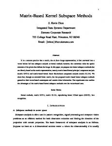
variance obtained from 500 Monte Carlo runs. Each experiment has been performed using N = 1000 data points. The future and past horizon have been chosen (somewhat arbitrarily) as follows: t − t0 = 5 and T − t = 5 for the ARX example and t − t0 = 10, T − t = 5 for the ARMAX one. Note that in this second case A¯2 = A2 − K2 C2 = 0.5 − 1 = −0.5 6= 0 and therefore strictly speaking the results of the paper do not apply. However the past horizon t − t0 is chosen equal to 10 so that 10 ' 9.8 · 10−4 is negligible to all practical purposes. A¯10 2 = (−0.5)

The experimental results show that indeed the variance computed using the formulas of this paper is in very good agreement with the sample variance obtained from the simulations. The original algorithm by Jansson [30] is indistinguishable from the “geometric version” called “whitening filter” in this paper. The asymptotic variance of “whitening filter” (computed using the formulas of this paper and estimated from the simulations) is indistinguishable from the Cram´er-Rao lower bound for the first three examples. In the ARMAX case with colored reference the Cram´er-Rao lower bound is instead smaller than the asymptotic variance for both algorithms analyzed in this paper (see figure 2, right plot). The interested reader may find in [10] an analysis of the “whitening filter” approach in the feedback free case. X. C ONCLUSIONS We have derived the asymptotic covariance of the system parameters estimated by (a version of) the algorithms proposed in [40], [30], [17] under a simplifying assumption. The tools developed in this paper allows however to deal with the general case ((t − t0 ) finite and no assumptions on A¯ or on the feedback channel), which we postpone to future work. In fact if the nilpotency assumptions are not satisfied,

July 14, 2005

DRAFT

30

White Reference

Colored Reference

Asymptotic Variance vs. Sample Variance

1

Asymptotic Variance vs. Sample Variance

0

10

10

0

10

Transfer function variance

Transfer function variance

−1

−1

10

10

−2

10

−2

10

−3

10

Fig. 1.

−3

0

0.5

1

1.5 2 normalized frequency ω

2.5

3

10

0

0.5

1

1.5 2 normalized frequancy ω

2.5

3

EXAMPLE 1 (ARX of order 1): Asymptotic Variance and Sample Variance (Monte Carlo estimate) vs. normalized

frequency (ω ∈ [0, π]) Solid with triangles (4) PEM, dashed with stars (∗): “innovation-estimation”, dashed with crosses (+): “whitening-filter” algorithm , dotted with circles (o): Jansson’s algorithm, dotted with crosses (+): asymptotic variance for “whitening-filter”, dotted with stars (∗): asymptotic variance for “innovation-estimation”, dotted with triangles (4): Cram´er Rao lower bound.

˜wf the estimators will be (asymptotically) biased (A˜ql ∞ 6= 0, A∞ 6= 0, etc.) and the deviation from the

asymptotic values described by more complicated expressions (see Propositions 7.1 and B.4). However, as some simulation results confirm, the approximation is reasonable also the system is not of the ARX type. A PPENDIX A £ ¤ ˆ ˆ Proof of Lemma 8.2. Recall that, since ²ˆN (t) ∈ Z[t0 ,t) , ²ˆN (t) = E ˆN (t) | Z[t0 ,t) . kG[t,T ] ²

Therefore, using the definition of vN in (51) we can write (∆vx )N from Proposition 6.1 in compact form as follows: (∆vx )N

£ + ¤ ˆ −L Hs E ˆ ˆ = Γ ˆN | Z[t0 ,t+1) + N kG[t+1,T ] ² ³ ´ £ + ¤ ql ˆ −L Hs E ˆ ˆ + KN [I 0] − Aˆql Γ ˆN | Z[t0 ,t) = N N kG[t,T −1] ² ¤ £ + ¤ £ + ˆ ql E ˆ ˆ ˆ ql E ˆ ˆ | Z | Z + M ² ˆ = M ² ˆ [t ,t+1) [t ,t) x1 x2 kG 0 0 N N kG[t,T −1] [t+1,T ]

(A.79)

ˆ ql , M ˆ ql . where the last equality defines M x2 x1

July 14, 2005

DRAFT

31

White Reference

Colored Reference

Asymptotic Variance vs. Sample Variance

1

Asymptotic Variance vs. Sample Variance

0

10

10

0

10

Transfer function variance

Transfer function variance

−1

−1

10

10

−2

10

−2

10

−3

10

Fig. 2.

−3

0

0.5

1

1.5 2 normalized frequency ω

2.5

3

10

0

0.5

1

1.5 2 normalized frequency ω

2.5

3

EXAMPLE 2 (ARMAX of order 1): Asymptotic Variance and Sample Variance (Monte Carlo estimate) vs. normalized

frequency (ω ∈ [0, π]) Solid with triangles (4) PEM, dashed with stars (∗): “innovation-estimation”, dashed with crosses (+) “whitening-filter” algorithm , dotted with circles (o): Jansson’s algorithm, dotted with crosses (+): asymptotic variance for “whitening-filter”, dotted with stars (∗): asymptotic variance for “innovation-estimation”, dotted with triangles (4): Cram´er Rao lower bound.

Similarly we have

³

(∆vy )N

´ £ + ¤ ql ˆ −L ˆ ˆ [I 0] − CˆN ΓN Hs · E ˆN | Z[t0 ,t) = kG[t,T −1] ² £ + ¤ ˆ yql E ˆ ˆ = M ˆN | Z[t0 ,t) kG[t,T −1] ²

=

(A.80)

ˆ yql . where the last equality defines M

Rewriting (A.79) as follows ¡ ¢ ¡ ¢ ˆ ql Σ ˆ ˆ −1 ˆ −1 + z[t ,t+1) ˆ ql ˆ ¯|g+ Σ (∆vx )N = M x1 ²ˆ+ z|g+ Σzz|g+ z[t0 ,t) N + Mx2 Σ²ˆ+ z 0 ¯z ¯|g z N ˆ we obtain the sample conditional covariance Σ ˆ as reported in (60). Similar calculations hold for ∆vx ξ|g

the other sample covariances.

¥

Proof of Proposition 8.3. We just need to recall that, for matrices of suitable dimensions vec (ABC) = ¡ > ¢ C ⊗ A vec (B); therefore from (60) we get, ³ ´   ˆ ²ˆ+ z|g+ Σ ˆ −1 + ³ ´ h h³ ´ i h³ ´ i i vec Σ zz|g −1 ˆ  ˆ> ˆ ql ˆ> ˆ ql ³ ´ . vec Σ = Σ−1 ⊗M Σ−1 ⊗M ˆ Σξˆξ|g ˆ x1 x1 ˆ ˆ ∆vx ξ|g ˆ Σzξ|g ˆ Σzξ|g ξˆξ|g ξˆξ|g −1 ˆ ˆ vec Σ²ˆ+ z¯|g+ Σz¯z¯|g+ July 14, 2005

DRAFT

32

From standard results (see [19]) the asymptotic properties of the right hand side do not change if we substih³ ´ i h³ ´ i ql ql ql −1 ˆ > −1 > ˆ tute the sample value of Σ ˆˆ Σzξ|g ⊗ Mx1 with its asymptotic value MA1 := Σ ˆˆ Σzξ|g ⊗ Mx1 . ˆ ˆ ξ ξ|g

ξ ξ|g

Similar considerations hold also for the other formulas in (60). ¥

Proof of Proposition 8.5. We shall prove only (72), the other expressions follow completely analogous. Recall that

and

´ ´ ³ ´ ³ ³ −1 −1 ˆ ˆ k k vec Σet+k z|g Σzz|gk = Σzz|gk ⊗ I vec Σet+k z|g

µ · ³ ´ ³ ´> ¸¶ h³ ´ i ˆ e z|gk = vec E ˆ eN (t + k) zgk ˆ zgk = E ⊗ e (t + k) . vec Σ N t+k [t0 ,t) [t0 ,t) N

N

Recalling that, given column vectors a, b, c, d, it holds that vec(a·b> )vec> (c·d> ) = (b⊗a)·(d> ⊗c> ) = (b · d> ) ⊗ (a · c> ) and using the assumption A1 (see formula (58)), some standard manipulations (see

[41]) yield (τ = h − k ) h³ ´ i h³ ´ iT ˆ zgk ˆ zgh lim N E{E ⊗ e (t + k) E ⊗ e (t + h) } = Σzgk zgh (τ ) ⊗ Λe . N N [t0 ,t) [t0 ,t) N →∞

N

N

¥

A PPENDIX B In this appendix we derive the asymptotic variance expressions for the “whitening filter” approach. The proof follows very closely the one for the “innovation estimation” algorithm and therefore only the main parts shall be reported without proof, which can be easily adapted from the parallel results established for the “innovation estimation” algorithm. A decomposition similar to that of Lemma 5.4 holds if, instead of (46) and (47), we use (48) and (49). Lemma B.1: Let us define,





   ˆ ¯ Hw (t, T − 1) :=    

0

0

...

0

ˆt CΨ .. .

0 .. .

... .. .

0 .. .

ˆt ... CΦ(t, T − 2)Ψ

July 14, 2005

      

ˆ T −2 0 CΨ

DRAFT

33



    ¯ s (t, T − 1) :=  H   

I

0

...

0

ˆt −C Θ .. .

I .. .

... .. .

0 .. .

ˆt ... −CΦ(t, T − 2)Θ

and



ˆ T −2 I −C Θ



   ¯ Hy (t, T −1) :=    

0

0

...

0

CK .. .

0 .. .

... .. .

0 .. .

CΦ(t, T − 2)K . . .

      





      

   ¯ Hu (t, T −1) :=    

0

0

...

0

CB .. .

0 .. .

... .. .

0 .. .

CΦ(t, T − 2)B . . .

CK 0

CB 0

Let us also define + ˆ (t, T − 1)w ¯ N (t) := H ¯ ˆN b w ˆ (t + 1, T )w ¯ (t + 1) := H ¯ ˆ+ b N

and

w

(B.81)

N

¯ s (t, T − 1)ˆ ¯ N (t) := H v ²+ N ¯ s (t + 1, T )ˆ ¯ N (t + 1) := H v ²+ N

(B.82)

+ Then the future output sequences yN := [yN (t)> , yN (t + 1)> , . . . , yN (T − 1)> ]> can be decomposed

as follows: + yN

¯ N (t) + v ¯ T − 1)ˆ ¯ N (t)+ = Γ(t, xN (t) − b ¯ u (t, T − 1)u+ + H ¯ y (t, T − 1)y+ + e ˆ+ +H N N N

(B.83)

and similarly y+ N

¯ N (t + 1) + v ¯ + 1, T )ˆ ¯ N (t + 1)+ = Γ(t xN (t + 1) − b ¯ u (t + 1, T )u+ + H ¯ y (t + 1, T )y+ + e ˆ+ +H N N N

(B.84)

Note that the dependence from the terms in Z[t,T ] and Z[t+1,T ] has a lower triangular structure. The state sequences ζˆN (t) and ζˆN (t + 1) are constructed according to (32). From equations (B.83) ¯ N and v ¯N (t) := ¯ N affect the state estimators. Defining Tˆ and (B.84) we can see how the error terms b ˆ¯ −L Γ(t ˆ¯ −L Γ(t, ¯ + 1, T ) a simple manipulation shows in fact that ¯ T − 1) and Tˆ¯ (t + 1) := Γ Γ N

N

N

¯N (t)ˆ ζˆN (t) = Tˆ xN (t) + ∆¯ xN (t)

(B.85)

¯N (t + 1)ˆ ζˆN (t + 1) = Tˆ xN (t + 1) + ∆¯ xN (t + 1)

(B.86)

and

July 14, 2005

DRAFT

      

34

where18 £ ¤ ˆ −L £ ¤ ˆ¯ −L E ¯ N (t) | Z[t ,t) + Γ ˆkZ ¯ E ˆkZ ¯ N (t) | Z[t0 ,t) ∆¯ xN (t) = −Γ v b [t,T −1] 0 [t,T −1] N N

and £ ¤ ˆ −L £ ¤ ˆ¯ −L E ¯ N (t + 1) | Z[t ,t+1) + Γ ˆkZ ¯ E ˆkZ ¯ N (t + 1) | Z[t0 ,t+1) ∆¯ xN (t + 1) = −Γ b v [t+1,T ] 0 [t+1,T ] N N

These decompositions are the starting point for obtaining recursions for ζˆN (t) involving the system parameters. The result, which we summarize in the next Proposition, follows from (B.85), (B.86) and Proposition 5.3. wf wf ˆ ˆ−1 ˆ ˆ−1 Proposition B.2: Let Awf N := TN (t + 1)ATN (t + 1), BN := TN (t + 1)B , CN := C TN (t + 1), wf wf wf wf KN := TˆN (t + 1)K , A¯wf N := AN − KN CN be the state matrices in the (data dependent) basis

TˆN (t + 1) and ¯ x )N (∆b

(∆¯ vx )N ¯ y )N (∆b (∆¯ vy )N

£ ¤ ˆ¯ −L E ¯ N (t + 1) | Z[t ,t+1) + ˆkZ := Γ b [t+1,T ] 0 N £ ¤ ¯ ¯ˆ −L ˆ ˆ ˆ ˆ N (t) −Awf N ΓN EkZ[t,T −1] bN (t) | Z[t0 ,t) − TN (t + 1)Ψt w £ ¤ ¯ˆ −L E ˆkZ ¯ N (t + 1) | Z[t0 ,t+1) + := Γ v [t+1,T ] N £ ¤ wf ¯ˆ −L ˆ ¯ N (t) | Z[t0 ,t) + KN −Awf ²ˆN (t) N ΓN EkZ[t,T −1] v £ ¤ wf ¯ ˆ −L E ¯ N (t) | Z[t ,t) ˆkZ := −CN Γ b [t,T −1] 0 N £ ¤ wf ¯ −L ˆ ˆ ¯ (t) | Z := ²ˆ (t) − C Γ E v N

N

N

kZ[t,T −1]

N

[t0 ,t)

wf wf ˆ t and ∆TˆN := TˆN (t + 1)Tˆ−1 (t), the estimated state sequences Defining KN (t) := KN + TˆN (t + 1)Θ N

ζˆN (t) and ζˆN (t + 1) satisfy the following recursion:  wf wf  ˆ  ζˆN (t + 1) = Awf eN (t)+  N ζN (t) + BN uN (t) + KN (t)ˆ     ¯ x )N + (∆¯ ˆ ˆ −(∆b vx )N + Awf N (I − ∆TN )ζN (t) (B.87) wf ˆ   ˆ y (t) = C ζ (t) + e (t) N N  N N    wf  ¯ −(∆by )N + (∆¯ vy )N + CN (I − ∆TˆN )ζˆN (t) ˜ wf ˜ wf The errors A˜wf N , BN , CN follows from the relation above similarly to the “innovation estimation”

algorithm presented in the main part of the paper. The main difference regards the presence in the error of a term originating from the different choice of basis TˆN (t) and TˆN (t + 1). £ ¤ £ ¤ ˆkZ ˆkZ These expressions rely on the fact that E ²ˆN (t + k) | Z[t0 ,t) = E ²ˆN (t + k) | Z[t0 ,t) and [t,T ] [t,t+k) £ ¤ £ ¤ ˆkZ ˆkZ ˆ N (t + k − 1) | Z[t0 ,t) = E ˆ N (t + k − 1) | Z[t0 ,t) . The first is proved in Lemma B.6, while the second E w w [t,T ] [t,t+k) 18

is left to the reader.

July 14, 2005

DRAFT

35

¯ x )N +(∆¯ ¯ y )N + ˆ ˆ Proposition B.3: Let (∆¯ x)N := −(∆b vx )N +Awf y)N := −(∆b N (I−∆TN )ζN (t) and (∆¯ wf ˜ wf ˜ wf (∆¯ vy )N +CN (I −∆TˆN )ζˆN (t). The error matrices A˜wf N , BN , CN obtained solving (33) (or equivalently

(B.87)) satisfy A˜wf N

ˆ ˆ Σ ˆ −1 = Σ ∆¯ xζ|g ˆˆ

˜ wf B N

ˆ ˆ −1 = Σ ˆ e) Σ ∆¯ xu|(ζ,ˆ

ζ ζ|g ˆ e) uu|(ζ,ˆ

(B.88)

wf ˆ ˆΣ ˆ −1 C˜N = Σ ∆¯ yζ ζˆζˆ Proof: The proof follows the same lines as that of Proposition 6.2 and will be omitted.

Unfortunately the analysis of the “whitening filter” based method is complicated by the fact that the estimated states at time t and time t + 1 correspond in general to different choice of basis (see equations (B.85) and (B.86)) which is reflected in (B.87) by the terms containing (I − ∆TˆN ). This difference unfortunately does not even disappear as N → ∞ and therefore contributes to the “bias” term. Under the simplifying assumption that A¯ is nilpotent then TˆN (t) = TˆN (t + 1). The same equality holds asymptotically if t − t0 increases at a suitable rate with N . Remark B.8 To the author’s experience both the bias and the fluctuations introduced by the factor ∆TˆN seem to have only marginal effect. A somewhat qualitative explanation of this statement could be as follows. The matrices19 CΦ(t, t + k) and CΦ(t + 1, t + 1 + k) which constitute the k -th block row ¯ T − 1) and Γ(t ¯ + 1, T ) contain in corresponding positions time varying matrices of respectively Γ(t, K(s) and K(s + 1) which satisfy Riccati-type recursions. If the Riccati recursion is in steady state, i.e. ¯ T − 1) = Γ(t ¯ + 1, T ). In the non steady-state conditions it K(s) = K(s + 1) ∀ s > t − t0 then Γ(t,

may still be reasonable to assume that one iteration of the Riccati equation does not change things too much. Of course this is just a qualitative statement, but somehow explains the experimental results in [17] where satisfying results are obtained also when the eigenvalues of A − KC are close to the unit circle provided those of F − LH are nearly zero (see simulation Example 4 in [17]).

♦

˜ wf ˜ wf Proposition B.4: Let ∆T := ∆Tˆ∞ and ∆T˜N := ∆T − ∆TˆN . Then the error matrices A˜wf N , B N , CN ˜wf ˜wf ˜ wf ˜ wf ˜ wf ˜ wf ˜ wf ˜ wf admit the decompositions A˜wf N = A∞ + ∆AN , BN = B∞ + ∆BN , CN = C∞ + ∆CN where wf −1 A˜wf ∞ = −Σ∆b ¯ x ζ|g ˆ Σ ˆˆ + A∞ (I − ∆T ) wf ˜∞ B

=

wf C˜∞ =

19

Recall that Φ(t, s) :=

July 14, 2005

Qs−1−t i=0

ζ ζ|g −1 −Σ∆b¯ x u|(ζ,ˆ ˆ e) Σuu|(ζ,ˆ ˆ e) wf −Σ∆b¯ y ζˆΣ−1 ˆx ˆ + C∞ (I x

− ∆T )

(A − K(s − 1 − i)C).

DRAFT

36

and

∆A˜wf N ˜ wf ∆B N wf ∆C˜N

· −1 ˜ ¯ ˆ Σ−1 + A˜wf ˆ ˜ ˆ Σ−1 + Σ = Σ ∞ Σζˆζ|g ˆ Σ ˆˆ + ˆˆ ∆bx ζ|g ˆˆ ∆¯ vx ζ|g ζ ζ|g wf +A∞ ∆T˜N +

(Awf N

−

ζ ζ|g wf A∞ )(I −

ζ ζ|g

∆T )

· −1 ˜ ¯ = Σ ˆ e) Σ ∆bx u|(ζ,ˆ ·

=

−1 ˜ wf ˜ ˆ e) Σuu|(ζ,ˆ ˆ e) ˆ e) + B∞ Σuu|(ζ,ˆ uu|(ζ,ˆ wf ˜ −1 ˜ ¯ ˆΣ−1 + C˜∞ ˆ Σ ΣζˆζˆΣ−1 +Σ ∆by ζ ζˆζˆ ∆¯ vy ζˆΣζˆζˆ + ζˆζˆ wf wf wf +C∞ ∆T˜N + (CN − C∞ )(I − ∆T )

−1 ˆ +Σ ˆ e) Σ ∆¯ vx u|(ζ,ˆ

ˆ e) uu|(ζ,ˆ

·

where = denotes equality up to terms which are o( √1N ) in probability20 . Note that in this case the following parts of the error √ ˜ ˆ Σ−1 + Awf ∆T˜N + (Awf − Awf )(I − ∆T ) ˜ ¯ ˆ Σ−1 + A˜wf Σ N (Σ ∞ ζˆζ|g ∞ ∞ N ˆ ˆ ∆bx ζ|g ζˆζ|g ζˆζ|g √ −1 −1 ˜ ¯ ˜ wf ˜ N (Σ ˆ e) Σuu|(ζ,ˆ ˆ e) Σuu|(ζ,ˆ ˆ e) + B∞ Σuu|(ζ,ˆ ˆ e) ) ∆bx u|(ζ,ˆ √ wf wf ˜ wf wf ˜ ¯ ˆΣ−1 + C˜∞ ˜ N (Σ ΣζˆζˆΣ−1 ˆˆ + C∞ ∆TN + (CN − C∞ )(I − ∆T )) ∆by ζ ˆˆ ζζ

ζζ

go to zero in probability when A¯t−t0 → 0 at a suitable rate (see [8]) with N . Under this condition only the terms related to ∆¯ vx and ∆¯ vy have to be accounted for variance. Both this approach and the computation of the variance in the general case (for t − t0 finite) would introduce further technical complications. For reasons of space and ease of exposition we prefer at this point to make the assumption that ˜ wf ˜ wf A¯t−t0 = 0 holds. This, as we have shown in [17], implies that A˜wf ∞ = 0, B∞ = 0, C∞ = 0 (and also ¢ ¢ ¡ ¡ ¯y ¯x = 0, ∆TˆN = ∆T = I); see Proposition B.2, Lemma 5.2 and equation (B.81). = 0, ∆b ∆b N N

Recall now that under the assumption that A¯t−t0 = 0 ˜wf A˜wf N = ∆AN ˜ wf = ∆B ˜ wf B N N wf C˜N

=

wf ∆C˜N

· −1 ˆ = Σ ˆ Σ ˆˆ ∆¯ vx ζ|g

ζ ζ|g

·

−1 ˆ = Σ ˆ e) Σ ∆¯ vx u|(ζ,ˆ

ˆ e) uu|(ζ,ˆ

·

=

−1 ˆ Σ ∆¯ vy ζˆΣζˆζˆ

ˆ ˆ ˆ we just need to study the asymptotic properties of Σ ˆ , Σ∆¯ ˆ e) and Σ∆¯ ∆¯ vx ζ|g vx u|(ζ,ˆ vy ζˆ. ¯ := Proposition B.5: Let introduce the shorthands z+ := z[t,T −1] , z+ := z[t+1,T ] , z := z[t0 ,t) , z ³ ´ wf wf wf wf wf −L −L ˆ ˆ ˆ ¯ ¯ ˆ ¯ ¯ ˆ z[t ,t+1) . Let M := x1 := KN [I 0] − AN ΓN Hs (t, T − 1) , Mx2 := ΓN Hs (t + 1, T ) and My ´ ³ 0 wf ¯ −L ˆ H ¯ (t, T − 1) . [I 0] − C Γ N

N

s

Let as usual denote the asymptotic values (in probability as N → ∞ ) of matrices removing the “hat” wf ˆ wf ) and let from the symbol denoting the sample version21 (e.g. Mx2 := limN →∞ M x2 20

wf wf wf wf wf We remind the reader that Awf which correspond to the ∞ , B∞ , C∞ denote the asymptotic values of AN , BN , CN

asymptotic choice of basis in (32) for N → ∞. 21

We refer the reader to Remark VIII.7 concerning the issue of convergence.

July 14, 2005

DRAFT

37

wf MA1

:=

wf MA2

:=

wf MB1

:=

wf MB2

:=

MCwf

:=

h³ ´ i wf > Σ−1 Σ ⊗ M x1 ˆ ˆˆ h³ ζ ζ|g z¯ζ|g ´ i wf −1 > Σ ˆˆ Σzζ|g ⊗ M x2 ˆ h³ ζ ζ|g ´ i wf Σ−1 ˆ Σ> ⊗ M x1 ˆ i h³ uu|(ζ,ˆe) zu|(ζ,ˆe) ´ wf −1 > ⊗ M Σ Σ x2 ˆ ˆ h³ uu|(ζ,ˆe) ´ z¯u|(ζ,ˆe) i wf −1 Σ ˆ ˆ Σ> ⊗ My zζˆ

(B.89)

ζζ

Then the following first order approximation (up to o( √1N ) terms in probability) of vectorized sample covariances can be used to compute the asymptotic distribution: ´   ³ ˆ −1 + ˆ ²ˆ+ z|z+ Σ ³ ´ h i vec Σ · zz|z −1 wf wf ˆ  ³ ´  = MA1 vec Σ MA2 ˆ Σζˆζ|z ˆ ∆¯ vx ζ|g −1 ˆ ˆ vec Σ²ˆ+ z¯|z+ Σz¯z¯|z+ ´   ³ ˆ ²ˆ+ z|z+ Σ ˆ −1 + ³ ´ h i vec Σ (B.90) · zz|z −1 wf wf ˆ  ³ ´  vec Σ ˆ e) Σuu|(ζ,ˆ ˆ e) = MB1 MB2 ∆¯ vx u|(ζ,ˆ ˆ ²ˆ+ z¯|z+ Σ ˆ −1 + vec Σ ¯z ¯|z z ³ ´ ³ ´ · wf −1 −1 ˆ ˆ ˆ vec Σ ∆¯ vy ζˆΣζˆζˆ =MC vec Σ²ˆ+ z|z+ Σzz|z+ Proof: Since the proof of this proposition follows the same lines of the proof of Lemma 8.2 and Proposition 8.3 it will be omitted. The last effort left is to compute the asymptotic covariance of  ³ ´  ˆ ²ˆ+ z|z+ Σ ˆ −1 + vec Σ zz|z  ´  ³ ˆ −1 + ˆ ²ˆ+ z¯|z+ Σ vec Σ

(B.91)

¯z ¯|z z

Using the same permutation matrices P and P¯ defined in (64) it is possible to write (B.91) in terms n o o n ˆ −1 + for i = 1, .., T − t. ˆ ²ˆ z|z+ Σ ˆ −1 + , i = 0, .., T − t − 1 and vec Σ ˆ ²ˆ z¯|z+ Σ of vec Σ t+i t+i ¯z ¯|z z zz|z An instrumental result is the following:

£ ¤ ˆkZ Lemma B.6: The oblique projection E ²ˆN (s + k) | Z[t0 ,s) satisfies the following: [s,T ] £ ¤ £ ¤ ˆkZ ˆkZ E ²ˆN (s + k) | Z[t0 ,s) = E ²ˆN (s + k) | Z[t0 ,s) = [s,T ] [s,s+k−1] £ ¤ ˆkZ = E eN (s + k) | Z[t0 ,s) . [s,s+k−1]

(B.92)

Let define the shorthands zk := z[t,t+k) and zk := z[t+1,t+k) . Then (B.92) is equivalent to the equation for the coefficients ˆ ²ˆ z|z+ Σ ˆ −1 + Σ t+k zz|z

ˆ e z|zk Σ ˆ −1 k ˆ ²ˆ z|zk Σ ˆ −1 k = Σ = Σ t+k t+k zz|z zz|z

(B.93)

ˆ z¯z¯|z+ ˆ ²ˆ z¯|z+ Σ Σ t+k

ˆ ²ˆ z¯|zk Σ ˆ −1 k = Σ ˆ e z¯|zk Σ ˆ −1 k = Σ t+k t+k ¯z ¯|z ¯z ¯|z z z

(B.94)

and

July 14, 2005

DRAFT

38

ˆ N (t + k) | Z[t ,t+k) ] Proof: The proof follows easily from the fact that ²ˆN (t + k) = E[e 0

It follows from (B.93) and (B.94) and the discussion after formula (B.91) that the asymptotic variance we are seeking can be expressed in terms of variances and covariances of terms of the form √ √ √ ˆ wf := N Σ ˆ e z|zk Σ−1 k =· N Σ ˆ e z|zk Σ ˆ −1 k NR t+k t+k k zz|z zz|z

and

√ √ √ ˆ¯ wf := N Σ ˆ e z¯|zk Σ−1 k =· N Σ ˆ e z¯|zk Σ ˆ −1 k NR t+k t+k k ¯z ¯|z ¯z ¯|z z z

k = 0, . . . , T − t − 1

k = 1, . . . , T − t

which we compute in the next proposition. Proposition B.7: Let us assume that the assumptions A1 and A2 hold. Let us define h i ⊥ zzk := E z | Z [t +τ,t+τ ) 0 [t0 +τ,t+τ ) [t+τ,t+τ +k] , h i ⊥ ¯zk z := E z | Z [t +τ,t+1+τ ) 0 [t0 +τ,t+1+τ ) [t+1+τ,t+τ +k] , · ³ ´> ¸ zk zh Σzzk zzh (τ ) := E z[t0 +τ,t+τ ) z[t0 ,t) . Similar definitions hold for Σz¯zk z¯zh (τ ) and Σzzk z¯zh (τ ). Let also23 Qwf := k ´ ³ Σ−1 ¯z ¯|zk ⊗ I and τ := h − k , then: z

22

³ ´ ¯ wf := Σ−1 ⊗ I , Q k k zz|z

³ ´ √ ³ ´ ³ ´> √ ˆ wf , N vec R ˆ wf } = Qwf (Σzzk zzh (τ ) ⊗ Λe ) Qwf Σwf (k, h) := AsCov { N vec R 11 k h k h

(B.95)

Similarly ³ ´ ³ ´ ³ ´> √ ˆ¯ wf , √N vec R ˆ ¯ wf } = Q ¯ wf (Σz¯zk z¯zh (τ ) ⊗ Λe ) Q ¯ wf N vec R Σwf (k, h) := AsCov { 22 k h k h

(B.96)

As far as the cross terms are concerned, we have ³ ´ √ ³ ´ ³ ´> √ ˆ ˆ wf , N vec R ¯ wf } = Qwf (Σzzk z¯zh (τ ) ⊗ Λe ) Q ¯ wf Σwf 12 (k, h) := AsCov { N vec Rk h k h

(B.97)

Proof: It is essentially analogous to the proof of Proposition 8.5 and for reasons of space will be omitted. Defining



Σwf 11 (0, 0) .. .

  Σwf :=  11 

... .. .

Σwf 11 (T − t − 1, 0) . . . zk

22

The superscript

23

Note that Σzz|zk = Σzzk zzk (0).

July 14, 2005

Σwf 11 (0, T − t − 1) .. .

   , 

(B.98)

Σwf 11 (T − t − 1, T − t − 1)

is meant to remind that the process z is taken conditionally on the k lags of the joint future.

DRAFT

39



Σwf 22 (1, 1) .. .

  Σwf :=  22 

Σwf 22 (T − t, 1) . . . 

and

  Σwf 12 :=  

Σwf 22 (1, T − t) .. .

... .. .

Σwf 12 (0, 1) .. .

  , 

(B.99)

Σwf 22 (T − t, T − t) 

Σwf 12 (0, T − t) .. .

... .. .

Σwf 12 (T − t − 1, 1) . . .



  , 

(B.100)

Σwf 12 (T − t − 1, T − t)

from Proposition B.7 it follows that  ´    ³ ˆ ²ˆ+ z|z+ Σ ˆ −1 +  √ vec Σ P zz|z ³ ´  = AsVar N   ˆ ²ˆ+ z¯|z+ Σ ˆ −1 + 0 vec Σ ¯z ¯|z z



 wf Σwf Σ P 12   ³ 11´>  Σwf Σwf P¯ 0 12 22 0

0 P¯

> 

(B.101) Collecting the results obtained so far we have basically proven the main result of the paper. Proof of Theorem 8.1. [Whitening filter approach]

³ ´ √ For convenience we report, before starting the proof, the asymptotic variance formulas for N vec A˜wf N , ³ ´ ³ ´ √ √ ˜ wf and N vec C˜ wf . The formulas are the same as those reported in Theorem 8.1 for N vec B N N

the “innovation estimation” algorithm, provided we substitute the superscript

ql

with the superscript

wf .

Letting 

wf MA1 P

  wf M wf :=  MB1 P  MCwf P

then

³ ´   ˜wf  vec A  N  √  ³ ´  ˜ wf AsVar N  vec B N   ³ ´   wf  ˜ vec CN



wf ¯ MA2 P

 wf ¯  MB2 P   0

     wf wf   Σ Σ ¡ ¢ 11 12   M wf >  = M wf  ³ wf ´> wf   Σ12 Σ22  

(B.102)

Recalling now that under the assumption that A¯t−t0 = 0 ˜wf A˜wf N = ∆AN ˜ wf = ∆B ˜ wf B N N wf wf C˜N = ∆C˜N

· −1 ˆ = Σ ˆ Σ ˆˆ ∆¯ vx ζ|g

ζ ζ|g

·

−1 ˆ = Σ ˆ e) Σ ∆¯ vx u|(ζ,ˆ

ˆ e) uu|(ζ,ˆ

·

−1 ˆ = Σ ∆¯ vy ζˆΣ ˆˆ ζζ

asymptotic normality follows again from standard results on asymptotic properties of sample covariances [41][p. 550]. Using Propositions B.5, B.7 and equation (B.101) the asymptotic variance formula follows. July 14, 2005

DRAFT

40

¥ ˆ s = 0 ∀s ≥ t. This Remark B.9 It is worth noting that under the stated assumption that A¯t−t0 = 0 also Θ ¯ s (t, T − 1) = H ¯ s (t + 1, T ) = I which simplifies significantly the variance expressions. The implies that H ˆ t disappears. The same reason for this simplification is that, in the state recursion (48) the term due to Θ

does not happen for the “innovation estimation” algorithm. We believe this may be the starting point for further analysis of these formulas. For reasons of space we postpone this discussion to future work. ♦

ACKNOWLEDGMENT The author would like to thank Giorgio Picci for many discussions on the subject and for his continuing support and encouragement over these years and the colleagues in Padova for suggestions on how to improve the manuscript. The author is indebted with the editor (L. Ljung) of the special issue to which the paper was originally submitted and with the reviewers for their careful reading and many insightful comments. R EFERENCES [1] D. Bauer, “Some asymptotic theory for the estimation of linear systems using maximum likelyhood methods or subspace algorithms,” Ph.D. dissertation, TU Wien, Austria, 1998. [2] ——, “Comparing the cca subspace method to pseudo maximum likelihood methods in the case of no exogenous inputs,” Journal of Time Series Analysis (submitted), 2002. [3] ——,

“Subspace

algorithms,”

2003,

slides

of

the

Semiplenary

Lecture

given

at

SYSID,

available

at

www.sysid2003.nl/plenaries/sp4.pdf. [4] ——, “Subspace methods,” in Proc.of IFAC Symposium on System Identification, Rotterdam, The Netherlands, August 2003, pp. 763–773. [5] ——, “Asymptotic properties of subspace estimators,” Automatica, vol. 41, pp. 359–376, 2005. [6] D. Bauer, M. Deistler, and W. Scherrer, “On the impact of weighting matrices in subspace algorithms,” in Proceedings of IFAC International Symposium on System Identification, Santa Barbara, June 2000, p. N.A. [7] D. Bauer and M. Jansson, “Analysis of the asymptotic properties of the moesp type of subspace algorithms,” Automatica, vol. 36, pp. 497–509, 2000. [8] D. Bauer and L. Ljung, “Some facts about the choice of the weighting matrices in larimore type of subspace algorithm,” Automatica, vol. 36, pp. 763–773, 2001. [9] P. Caines and C. Chan, “Estimation, identification and feedback,” in System Identification: Advances and Case Studies, R. Mehra and D. Lainiotis, Eds.

Academic, 1976, pp. 349–405.

[10] A. Chiuso, “On the relation between cca and predictor based subspace identification,” in submitted to CDC-ECC 2005, 2005, available at http://www.dei.unipd.it/∼chiuso.

July 14, 2005

DRAFT

41

[11] A. Chiuso and G. Picci, “Constructing the state of random processes with feedback,” in Proc. of the IFAC Int. Symposium on System Identification (SYSID), Rotterdam, August 2003. [12] ——, Geometry of Oblique Splitting, Minimality and Hankel Operators, ser. Lect. Notes in Control and Information Sciences.

Springer, 2003, no. 286, pp. 85–124.

[13] ——, “The asymptotic variance of subspace estimates,” Journal of Econometrics, vol. 118, no. 1-2, pp. pp. 257–291, 2004. [14] ——, “Asymptotic variance of subspace methods by data orthogonalization and model decoupling: A comparative analysis,” Automatica, vol. 40, no. 10, pp. pp. 1705–1717, 2004. [15] ——, “Numerical conditioning and asymptotic variance of subspace estimates,” Automatica, vol. 40, no. 4, pp. pp. 677–683, 2004. [16] ——, “On the ill-conditioning of subspace identification with inputs,” Automatica, vol. 40, no. 4, pp. pp. 575–589, 2004. [17] ——, “Consistency analysis of some cloded-loop subspace identification methods,” Automatica, vol. 41, no. 3, pp. 377–391, 2005. [18] C. T. Chou and M. Verhaegen, “Closed-loop identification using canonical correlation analysis,” in Proceedings of the European Control Conference, Karlsruhe, 1999, pp. CD–ROM, F162. [19] T. Ferguson, A Course in Large Sample Theory. Chapman and Hall, 1996. [20] U. Forsell and L. Ljung, “Closed loop identification revisited,” Automatica, vol. 35, pp. 1215–1242, 1999. [21] M. Gevers, L. Ljung, and P. V. den Hof, “Asymptotic variance expressions for closed-loop identification,” Automatica, vol. 37, no. 5, pp. 781–786, 2001. [22] M. Gevers and B. Anderson, “Representation of jointly stationary feedback free processes,” Intern. Journal of Control, vol. 33, pp. 777–809, 1981. [23] ——, “On jointly stationary feedback-free stochastic processes,” IEEE Trans. Automat. Contr., vol. 27, pp. 431–436, 1982. [24] G. Golub and C. V. Loan, Matrix Computation, 2nd ed. The Johns Hopkins Univ. Press., 1989. [25] C. Granger, “Economic processes involving feedback,” Information and Control, vol. 6, pp. 28–48, 1963. [26] T. Gustafsson, “Subspace-based system identification: weighting and pre-filtering of instruments,” Automatica, vol. 38, pp. 433–443, 2002. [27] E. Hannan and M. Deistler, The Statistical Theory of Linear Systems. Wiley, 1988. [28] E. Hannan and D. Poskitt, “Unit canonical correlations between future and past,” The Annals of Statistics, vol. 16, pp. 784–790, 1988. [29] M. Jansson, “Asymptotic variance analysis of subspace identification methods,” in Proceedings of SYSID2000, S. Barbara Ca., 2000. [30] ——, “Subspace identification and arx modelling,” in Proceedings of SYSID 2003, Rotterdam, 2003. [31] M. Jansson and B. Wahlberg, “On consistency of subspace methods for system identification,” Automatica, vol. 34, pp. 1507–1519, 1998. [32] T. Katayama, H. Kawauchi, and G. Picci, “Subspace identification of closed loop systems by orthogonal decomposition,” To appear, Automatica (brief paper), 2003. [33] W. Larimore, “Canonical variate analysis in identification, filtering, and adaptive control,” in Proc. 29th IEEE Conf. Decision & Control, Honolulu, 1990, pp. 596–604. [34] W. Lin, S. Qin, and L. Ljung, “A framework for closed-loop subspace identification with innovation estimation,” Texas-Wisconsin Modeling and Control Consortium, Tech. Rep. 07, 2004, available at www.che.wisc.edu/jbr-group/techreports/twmcc-2004-07.pdf.

July 14, 2005

DRAFT

42

[35] A. Lindquist and G. Picci, “Canonical correlation analysis, approximate covariance extension and identification of stationary time series,” Automatica, vol. 32, pp. 709–733, 1996. [36] L. Ljung, System Identification; Theory for the User.

Prentice Hall, 1997.

[37] L. Ljung and T. McKelvey, “Subspace identification from closed loop data,” Signal Processing, vol. 52, no. 2, pp. 209–216, 1996. [38] M. Moonen, B. De Moor, L. Vandeberghe, and J. Vandewalle, “On- and off-line identification of linear state-space models,” Int. J. of Control, vol. 49, no. 1, pp. 219–232, 1989. [39] G. Picci and T. Katayama, “Stochastic realization with exogenous inputs and “subspace methods” identification,” Signal Processing, vol. 52, pp. 145–160, 1996. [40] S. Qin and L. Ljung, “Closed-loop subspace identification with innovation estimation,” in Proceedings of SYSID 2003, Rotterdam, 2003. [41] T. S¨oderstr¨om and P. Stoica, System Identification.

Prentice-Hall, 1989.

[42] A. C. Van der Klauw, M. Verhaegen, and P. P. J. Van den Bosch, “State space identification of closed loop systems,” in Proc. 30th IEEE Conf. on Dec. & Control, Brighton, U.K., 1991, pp. 1327–1332. [43] P. Van Overschee and B. De Moor, “Subspace algorithms for the stochastic identification problem,” Automatica, vol. 29, pp. 649–660, 1993. [44] ——, “N4SID: Subspace algorithms for the identification of combined deterministic– stochastic systems,” Automatica, vol. 30, pp. 75–93, 1994. [45] ——, Subspace Identification for Linear Systems.

Kluwer Academic Publications, 1996.

[46] ——, “Closed loop subspace systems identification,” in Proceedings of 36th IEEE Conference on Decision & Control, San Diego, CA, 1997, pp. pp. 1848–1853. [47] M. Verhaegen, “Application of a subspace model identification technique to identify lti systems operating in closed-loop,” Automatica, vol. 29, pp. 1027–1040, 1993. [48] ——, “Identification of the deterministic part of mimo state space models given in innovations form from input-output data,” Automatica, vol. 30, pp. 61–74, 1994. [49] M. Verhaegen and P. Dewilde, “Subspace model identification, part 1. the output-error state-space model identification class of algorithms; part 2. analysis of the elementary output-error state-space model identification algorithm,” Int. J. Control, vol. 56, pp. 1187–1210 & 1211–1241, 1992. [50] ——, “Subspace model identification, part 3. analysis of the ordinary output-error state-space model identification algorithm,” Int. J. Control, vol. 58, pp. 555–586, 1993. [51] M. Viberg, “Subspace-based methods for the identification of linear time-invariant systems,” Automatica, vol. 31, no. 12, pp. 1835–1851, 1995. [52] M. Viberg, B. Wahlberg, and B. Ottersten, “Analysis of state space system identification methods based on instrumental variables and subspace fitting,” Automatica, vol. 33, no. 9, pp. 1603–1616, 1997.

July 14, 2005

DRAFT