Attributed Typed Triple Graph Transformation with Inheritance in the Double Pushout Approach Esther Guerra Departamento de Inform´atica Universidad Carlos III de Madrid E-mail:
[email protected] Juan de Lara Escuela Polit´ecnica Superior, Ing. Inform´atica Universidad Aut´onoma de Madrid E-mail:
[email protected] 18th October 2006 Resumen Las gram´ aticas de grafos triples fueron propuestas por Andy Sch¨ urr con el objetivo de reescribir grafos triples [Sch¨ urr, 1994]. Son u ´tiles para mantener relaciones entre dos modelos que se est´ an manipulando. Este documento presenta una formalizaci´ on de las gram´ aticas de grafos triples basada en el enfoque algebraico Double Pushout. Comenzaremos definiendo un grafo triple en base al concepto de E − graf o propuesto en [Ehrig et al., 2004b], el cual nos permite tener atributos en nodos y relaciones. A continuaci´ on usaremos los resultados obtenidos en [Ehrig et al., 2004a], donde las categor´ıas y los sistemas de reemplazo de alto nivel (HLR) adhesivos se utilizan como marco para la transformaci´ on de grafos. De este modo, la mayor´ıa de los resultados obtenidos para la categor´ıa de los grafos pueden ser extrapolados y aplicados a cualquier categor´ıa HLR adhesiva. Por esta raz´ on nuestra formalizaci´ on demuestra que grafos triples y morfismos de grafo triples son una categor´ıa HLR adhesiva, demostrando para ello que grafos triples y morfismos de grafo triples son isomorfos a una categor´ıa coma. Adem´ as, extendemos la noci´ on de regla de gram´ atica de grafos triple con condiciones de aplicaci´ on, y con un concepto de herencia similar al propuesto en [Bardohl et al., 2004], pero permitiendo tambi´en herencia en relaciones. Abstract Andy Sch¨ urr proposed triple graph grammars with the purpose of rewriting triple graphs [Sch¨ urr, 1994]. They are useful as a means to maintain the relations between two models that are being manipulated. This document presents a formalization of triple graph grammars based on UC3M-TR-CS-06-01
1
the Double Pushout algebraic approach. We first start by defining triple graphs using the concept of E − graph proposed in [Ehrig et al., 2004b], which allows attributes in edges and nodes. Then, we use the results in [Ehrig et al., 2004a], which introduce adhesive high-level replacement (HLR) categories and systems as a framework for graph transformation. In this way, most results from the category of graphs are lifted to adhesive HLR categories. Therefore, our formalization uses the fact that triple graphs and triple morphisms can be shown to be an adhesive HLR category, by demonstrating that triple graphs and morphisms are isomorphic to a comma category. In addition, we provide triple graph grammar rules with application conditions, and with an inheritance concept similar to the one proposed in [Bardohl et al., 2004], but allowing also inheritance of edges.
1
Introduction
Graph transformation [Ehrig et al., 1999][Ehrig et al., 2006] is a formal, high level, graphical and declarative means to manipulate graphs. Graph transformation systems are made of a set of graph transformation rules, each having graphs in their left and right hand sides (LHS and RHS). In order to apply a rule to a graph (called host graph), an occurrence of the LHS should be found in it. If some is found, then the rule is applied by replacing such occurrence by the RHS. The theory of graph transformation has been developing in the last 30 years [Ehrig et al., 1999]. The available results allow checking if two rules can be applied in any order yielding the same result (parallel and sequential independence), to check confluence (if a graph transformation system is deterministic), to amalgamate rules together through a common part (concurrency theorem), to check termination (under certain circumstances [Ehrig et al., 2005b]), etc. See [Ehrig et al., 2006] for a comprehensive review of the main results. Andy Sch¨ urr proposed triple graph grammars (TGGs) with the purpose of rewriting triple graphs [Sch¨ urr, 1994]. These are structures made of three graphs called source, target and correspondence respectively. The latter is used to maintain relationships between the elements of the other two graphs. Triple graph grammars have been used for model transformation [Taentzer et al., 2005] (translation of models from a source to a target formalism) and have the potential to be incremental. We have also used triple graphs to model multi-view visual languages [Guerra et al., 2005] and to relate the concrete and abstract syntax of visual languages [Guerra and de Lara, 2004]. TGGs are becoming ever more popular as model-driven software development (MDSDM) techniques [Stahl and V¨olter, 2006] gain more attention. In MDSD, model to model and model to platform (i.e. code) transformations play a central role. The OMG promotes the model-driven architecture (MDA) [MDA] as a particular implementation of MDSD using some of the OMG’s standards: UML, MOF and QVT [QVT]. The latter is a specification of a language for queries, views and transformations. The language for transformations combines both imper-
UC3M-TR-CS-06-01
2
ative and declarative constructs, but it is not formally defined. It is our belief that the theory of TGGs has the potential to provide such formalization. The aim of this report is to extend and formalize the concept of triple graph grammar presented in [Sch¨ urr, 1994]. In this way, in the new extension, we consider attributes in nodes and edges of triple graphs, and allow nodes in the correspondence graph to have morphisms either to nodes or to edges of the other graphs, as well as to remain undefined. We consider typing of triple graphs by a triple type graph (similar to the concept of type graph [Corradini et al., 1996] or meta-model [Atkinson and K¨ uhne, 2002]). Type graphs are provided with node inheritance relations, in a similar way as done in [Bardohl et al., 2004]. Moreover, we also provide edge type inheritance. We formalize triple graph transformation using the double pushout approach [Ehrig et al., 2006]. This is done by proving that triple graphs are indeed an adhesive HLR category. Moreover, as we have inheritance in type graphs, we allow rules to have abstract elements in their LHS. In this way, these elements can be matched to an instance of their subtypes. For the theoretic discussions, we have followed and extended the works in [Ehrig et al., 2006] and [Bardohl et al., 2004]. Triple graph grammars techniques were proposed in [Sch¨ urr, 1994] a means to derive lower-level, operational rules from creation grammars (i.e. grammars that model the synchronized creation of elements in the source and target graphs). The derived lower-level operational rules perform forward or backwards translations, incremental updates or so called consitency observing analyzers. In the present work, we provide a richer graph concept and a formalization of triple graph transformation in the DPO approach. However, the algorithms for derivation of operational rules for this richer graphs we propose are up to future work. The rest of the document is organized as follows. Section 2 starts by presenting attributed typed graphs, which will be used later for our formalization of triple graphs. Section 3 formalizes triple graphs, with typing and attributes in nodes and edges. Section 4 shows how to build pushouts and pullbacks in this structure. These categorical constructions are needed in order to define graph transformation systems. Section 5 proves that the category of triple graphs and morphisms are indeed an adhesive HLR category. This means that we can use most of the theory of graph transformation systems, which has been lifted from graphs to HLR categories [Ehrig et al., 2004a]. Section 6 presents the basic concepts of graph transformation explicitly for triple graphs. Although this is not necessary, since one could follow the theory of HLR, we show it for illustrative purposes. Section 7 adds the inheritance concept to triple graphs. Finally, section 8 presents the conclusions.
2
Attributed Typed Graphs
In this section, we define node and edge attributed typed graphs, following the notion of E − graph developed in [Ehrig et al., 2004b]. These definitions are included here, as we will use them later in section 3 as a basis for triple graphs. E-graphs are extended graphs that allow attributes in both nodes and edges.
UC3M-TR-CS-06-01
3
Attribute values are stored in set VD , and two additional kind of edges model attribution: the node and edge attribution edges. The first ones allow nodes to have attributes, while the second ones model edge attributes. Definition 1 (E-graph, taken from [Ehrig et al., 2006]) An E-graph is a tuple G = (VG , VD , EG , EN A , EEA , (sourcej , targetj )j∈{G,N A,EA} ), where: • VG is a set of graph nodes. • VD is a set of data nodes. • EG is a set of graph edges. • EN A is a set of “node attribution” edges. • EEA is a set of “edge attribution” edges. • sourceG : EG → VG , targetG : EG → VG . • sourceN A : EN A → VG , targetN A : EN A → VD . • sourceEA : EEA → EG , targetEA : EEA → VD .
EO G
sourceG targetG
// V G O
sourceEA
sourceN A
EEAE EE EE E targetEA EE "
VD
EN A y y yy yy y| y targetN A
Figure 1: An E-graph. Figure 2 shows an example of E-graph (using a graphical representation) depicting a sequence diagram. The diagram consist of two objects with one activation box each. The activation boxes are connected by message “msg1”. Node ActivationBox1 receives the start message (i.e. the entry point of the diagram). In addition to E-graphs, we also define mappings between two E-graphs. An E-graph morphism is a tuple of set morphisms, one for each set in the E-graph (VG , VD , EG , EN A , EEA ). In addition, the structure of the E-graph should be preserved, that is, the sourcei and targeti functions should commute with the morphisms. Definition 2 (E-graph morphism, taken from [Ehrig et al., 2006]) i i i i i Given two E-graphs Gi = (VGi , VDi , EG , EN A , EEA , (sourcej , targetj )j∈{G,N A,EA} ), 1 2 with i = 1, 2, an E-graph morphism f : G → G is a tuple (fVG , fVD , fEG , fEN A , fEEA ) UC3M-TR-CS-06-01
4
"object1"
"class1"
oname1
"object2" oname2
class1
Object1
StartPoint
ActivationBox1
Data Nodes (V D ) Graph Edges (E G ) Node Attribution Edges (E NA )
objectLifeLine2
mname
message
name
Graph Nodes (V G)
class2
Object2
"msg1"
objectLifeLine1 startMessage
"class2"
ActivationBox2
Edge Attribution Edges (E EA )
type
"msg0"
synchronous
Figure 2: An E-graph representing a Sequence Diagram. with fVi : Vi1 → Vi2 and fEj : Ej1 → Ej2 with i ∈ {G, D}, j ∈ {G, N A, EA}, where f commutes for all source and target: • fVG ◦ source1G = source2G ◦ fEG • fVG ◦ target1G = target2G ◦ fEG • fEG ◦ source1EA = source2EA ◦ fEEA • fVD ◦ target1EA = target2EA ◦ fEEA • fVG ◦ source1N A = source2N A ◦ fEN A • fVD ◦ target1N A = target2N A ◦ fEN A f EG
1 EG O
source1G target1G
source1EA
E1 GF EABBB BB BB B! target1EA @A
// V 1 G O
fVG
source1N A
VD1
1 EN A || | | || 1 }|| targetN A
/ V2 G O
source2G target2G
fVD
2 / EG O source2EA
source2N A fEN A
$/
2 / E2 o EEA N AB BB | | BB || BB ||target2 B! | target2N A EA }| / V2
ED
D
f EEA
BC
Figure 3: An E-graph morphism. Figure 4 shows an example of E-graph morphism. Nodes and edges in the E-graphs have been provided with a numeric label for matching purposes. Note UC3M-TR-CS-06-01
5
that this is a non-injective morphism since graph nodes 2 and 3 have the same image. 1
StartPoint
2 startMessage 7
3 message 8
ActivationBox1
9 name 4
10 type 5
"msg0"
synchronous
ActivationBox2
11 mname 6
"msg1"
f V = {(1, 1’), (2, 2’), (3, 2’)} G
f V = {(4, 3’), (5, 5’), (6, 4’)} D f E = {(7, 6’), (8, 7’)} G
f E ={} NA
f E = {(9, 8’), (10, 10’), (11, 9’)} EA
1’
StartPoint
2’ startMessage 6’
ActivationBox
8’ name 3’
type 7’ message
"msg0"
mname
10’ 9’
4’
"msg1" 5’
synchronous
Figure 4: An E-graph morphism. E-graphs and E-graph morphisms form a category, where the former are the objects and the latter the arrows. It is indeed a category, as the identity arrow is the identity morphism, and the composition of morphisms is associative. Definition 3 (Category EGraph, taken from [Ehrig et al., 2006]) E-graphs together with E-graph morphisms form the category EGraph. Although E-graphs allow attributes in nodes and edges, we combine E-graphs together with an algebra over an appropriate signature in order to structure the attribute values (the elements of VD ). Having an algebra allows us to distinguish types (sorts like integer, string, and so forth) for attribution, as well as operations. Therefore, we assume that an E-graph has an associated data signature DSIG, which contains the appropriate declaration of sorts and operations. Some of the declared sorts will be used for attribution, and the carrier sets of the attribution sorts must be exactly the elements of VD . Please note that it may be possible to have an infinite number of elements in VD . Definition 4 (Attributed Graph, taken from [Ehrig et al., 2006]) Given a data signature DSIG = (SD , OPD ) which contains sorts for attri0 bution SD ⊆ SD , an attributedUgraph AG = (G, D) consists of an E-graph G and a DSIG − algebra D with s∈S 0 Ds = VD . D
Figure 5 shows an example of attributed graph AG = (G, D) representing a sequence diagram. It uses a data signature DSIG, which is defined as: DSIG = Char+String+ sorts : MessageType UC3M-TR-CS-06-01
6
opns : synchronous: → MessageType asynchronous: → MessageType destroy: → MessageType That is, sort M essageT ype declares three constants synchronous, asynchronous 0 = {String, M essageT ype}; and destroy. The data sorts used for attribution are SD Char is an auxiliary type. "object1":String
"class1":String
oname1
"object2":String
class1
oname2
Object1
startMessage
objectLifeLine2 message
ActivationBox1
name
mname
"msg0":String
class2
Object2
objectLifeLine1
StartPoint
"class2":String
"msg1":String
ActivationBox2 type
synchronous:MessageType
Figure 5: An attributed graph. We define attributed graph morphisms between two attributed graphs as a tuple of two mappings. The first one is an E-graph morphism, the second one is an algebra homomorphism. Definition 5 (Attributed Graph morphism, taken from [Ehrig et al., 2006]) Given two attributed graphs AGi = (Gi , Di ) with i = 1, 2, an attributed graph morphism f : AG1 → AG2 is a pair f = (fG , fD ) where fG : G1 → G2 is an E-graph morphism and fD : D1 → D2 is an algebra homomorphism, such 0 that the diagram in Figure 6 commutes for all s ∈ SD . Ds1Ä _
fD,s
/ D2 sÄ _
= ² VD1
fG,VD
² / V2 D
Figure 6: Condition for attributed graph morphisms. Note how, in Figure 6, the inclusion of Dsi in VDi is given by the definition of attributed graph. Attributed graphs and attributed morphisms form a category, where the former are the objects and the latter the arrows. As before, it is indeed a category as the identity arrow is the identity attributed morphism, and the composition of attributed morphisms is associative. UC3M-TR-CS-06-01
7
Definition 6 (Category AGraph, taken from [Ehrig et al., 2006]) Given a data signature DSIG as above, attributed graphs together with attributed graph morphisms form the category AGraph. For the typing of attributed graphs we use the concept of type graph [Corradini et al., 1996]. This can be modelled as a distinguished attributed graph AT G, which is attributed over the final DSIG−algebra Z. That is, the carrier sets of each sort in Z have a unique element, which is the type name. Note how, the concept of type graph is similar to the one of meta-model [Atkinson and K¨ uhne, 2002], but the latter includes inheritance, multiplicities and other constraints, possibly using a constraint language. In section 7 we extend (triple) type graphs with inheritance of nodes and edges. Definition 7 (Attributed Type Graph, taken from [Ehrig et al., 2006]) An attributed type graph is an attributed graph AT G = (T G, Z), where Z is the final DSIG − algebra with carrier sets Zs = {s} ∀s ∈ SD . Figure 7 shows an example of attributed type graph AT G = (T G, Z) for the definition of UML sequence diagrams, where Z is the final algebra for the signature DSIG = Char + String + M essageT ype used in the example corresponding to Figure 5. This type graph models the concrete syntax of sequence diagrams, that is, it is not equal to the UML 1.5 meta-model since this latter models the abstract syntax, but not the concrete one. Basically, the type graph declares objects that can be linked to activation boxes. Activation boxes can be linked through life lines and through messages. They can also be linked to objects through create messages. Finally, the sequence diagram should have a start point with a start message. lifeLine
StartPoint
startMessage name
String
Types for Graph Nodes (V G)
createMessage
ActivationBox message mname
type
Object
Data Nodes (V D )
objectLifeLine
Graph Edges (E G ) MessageType class oname
Node Attribution Edges (E NA ) Edge Attribution Edges (E EA )
Figure 7: Attributed type graph for Sequence Diagrams. Now, we define graphs conformant to a type graph. This notion is similar to the relation between a model and its meta-model. We say that a graph is conformant to a type graph (or is an instance of it) if there is an attributed morphism from the graph to the type graph. In fact, from now on, we will work with tuples where the first element is the graph itself and the second one the typing morphism. This indeed can be formalized as a slice category. Definition 8 (Attributed Typed Graph, taken from [Ehrig et al., 2006]) UC3M-TR-CS-06-01
8
An attributed typed graph over AT G is an object T AG = (AG, t) in the slice category AGraph/ATG, where AG = (G, D) is an attributed graph and t : AG → AT G is an attributed graph morphism called the typing of AG. Now, we define morphisms between attributed typed graphs. These are attributed morphisms with the restriction that the typing should be preserved from the source to the target graph. Definition 9 (Attributed Typed Graph morphism, taken from [Ehrig et al., 2006]) Given two attributed typed graphs T AGi = (AGi , ti ) over AT G, an attributed typed graph morphism f : (AG1 , t1 ) → (AG2 , t2 ) is an attributed graph morphism f : AG1 → AG2 such that t2 ◦ f = t1 as Figure 8 shows. AG1H HH 1 HHt HH HH # f AT ; G v v vv vv 2 v ² vv t AG2 Figure 8: Condition for attributed typed graph morphisms. Figure 9 shows an attributed typed graph (AG, t). Nodes and edges are labelled with its type (in the usual UML notation for instances). As stated before, attributed instance graphs can be infinite, since data set String for attribution is infinite and all the values have to be part of the graph. Otherwise, attribute computation is not possible. In the figure, we only show those data elements used for attribution. "object1":String
"class1":String
: oname
"object2":String
: class
: oname
: Object
: startMessage : name
"msg0":String
: class
: Object
: objectLifeLine
: StartPoint
"class2":String
: ActivationBox
: objectLifeLine : message
: mname
"msg1":String
: ActivationBox : type
synchronous:MessageType
Figure 9: Attributed typed graph, with respect to the attributed type graph in Figure 7. Attributed typed graphs and attributed typed morphisms form a category, where the former are the objects and the latter the arrows. As before, it is indeed UC3M-TR-CS-06-01
9
a category as the identity arrow is the identity attributed typed morphism, and the composition of attributed typed morphisms is associative. Moreover, it is built using a slice category construction. Definition 10 (Category AGraphATG , taken from [Ehrig et al., 2006]) Attributed typed graphs over an attributed type graph AT G, together with attributed typed graph morphisms, form the category AGraphATG .
3
Attributed Typed Triple Graphs
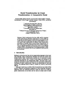
In this section, we use the previous concepts in order to formalize triple graphs. We start by defining the notion of TriE-graph, which is made of three E-graphs and two correspondence functions c1 and c2 . One of the three graphs is called correspondence graph. The correspondence functions are defined from the nodes in the correspondence graph to the nodes and edges in the other two graphs. In addition the functions can be undefined, what is modelled with a special element in the codomain (named “·”). Therefore, we have extended the actual notion of triple graphs [Sch¨ urr, 1994] in several ways. On the one hand, we use a definition that contemplates attributes in nodes and edges. On the other hand, our correspondence functions are more flexible as the codomain includes nodes, edges, and the special element for modelling that the function is undefined. Being able to relate links with both nodes and edges is crucial in our approach. Suppose we have two attributed edges between the same source and target nodes in the source graph, that we want to relate with other edges (also with attributes) in the target graph. Relating only the source and target nodes is not enough, as then we do not know which edge in the source graph is related to which one in the target graph. Therefore it is necessary to be able to directly map edges. This situation is depicted in Figure 10. To the left it is shown how mapping the source and target nodes is not enough, as we don’t know whether the edge with attribute ValueA is mapped to the edge with value 1 or 2. The situation is solved in the triple graph to the right by mapping the edges. On the other hand, as in [Guerra and de Lara, 2004], the source graph may represent the concrete syntax graph, and the target graph the abstract syntax. In this casen the user interacts with the concrete graph, and he may delete elements which are already related to elements in the abstract graph. When such operation is performed, the mapping of the correspondence node becomes undefined. Keeping the correspondence node with just one mapping is useful as we may later want to delete the element in the target graph, and probably some others related to it. Moreover, being able to know that a mapping is undefined is also a very useful negative test in triple graph grammar rules. Definition 11 (TriE-graph) A TriE-graph T riG = (G1 , G2 , GC , c1 , c2 ) is made of three E-graphs Gi = (VGi , VDi , EGi , EN Ai , EEAi , (sourceji , targetji )j∈{G,N A,EA} ) for i ∈ {1, 2, C}, with VD1 = VD2 = VDC , and two functions cj : VGC → VGj ∪ EGj ∪ {·} (for j = 1, 2). UC3M-TR-CS-06-01
10
2
2 slot
slot t1 :B
t2 :B
t1 :B
t2 :B slot
slot 1
1
c1:A
c2:A
c1:A
c3:D
"value A"
c2:A
"value A"
val s1 :C
c4:D
val s2 :C
val "value B"
s1 :C
s2 :C val "value B"
Figure 10: Insufficient Mapping of Nodes(left). Mapping of Edges (right) Graph G1 is called source, G2 is called target and GC is called correspondence. Functions c1 and c2 are called source and target correspondence functions respectively. We use the auxiliary sets edgesi = {x ∈ VGC |ci (x) ∈ EGi }, nodesi = {x ∈ VGC |ci (x) ∈ VGi } and undefi = {x ∈ VGC |ci (x) = ·} for i = 1, 2. The latter set is used to denote that the correspondence function ci for an element x is undefined. The previous two sets are used to denote that the codomain of the correspondence function ci for an element x are edges or nodes, respectively. Morphisms c1 and c2 represent m-to-n relationships between nodes and edges in G1 and G2 via GC in the following way: x ∈ VG1 ∪ EG1 is related to y ∈ VG2 ∪ EG2 ⇐⇒ ∃z ∈ VGC | x = c1 (z) and y = c2 (z). Note also that all the data sets VDi are assumed to be equal. We could have used just one set for each one of the three graphs, but having independent E-graphs makes it possible to reuse some of the concepts developed in [Ehrig et al., 2004b] for E-graphs. Figure 12 shows a TriE-graph for the definition of the abstract and concrete syntax of UML sequence diagrams. The target graph G2 in the upper part corresponds to the abstract syntax, the source graph G1 in the lower part corresponds to the concrete syntax, and finally, the correspondence graph GC in the middle contains elements relating G1 and G2 by means of the correspondence functions. Note that, although VD1 = VD2 = VDC , for clarity, we have represented the elements of these sets in each one of the E-graphs. However, the elements of the three sets are the same. Therefore, node “class100 in VD2 is the same as node “class100 in VD1 . Now, we define mappings between two TriE-graphs. These are made of three E-graph morphisms plus additional constraints regarding the preservation of the correspondence functions. Definition 12 (TriE-graph morphism) UC3M-TR-CS-06-01
11
{·} O O c1 |edges1 c1 |undef1
c1 |nodes1
EG1 O
|
sourceG1
// V G1 O
targetG1
y
sourceGC
EGC O
EEA1 EN A1 @@ ~ @@ ~ ~ @@ ~ ~ targetEA1 @Ã ~~~ targetN A1 VD1
c2 |nodes2
/E // V G C O c2 |edges2 GO 2
targetGC
sourceN AC
sourceN A1 sourceEAC
sourceEA1
c2 |undef2
sourceG2 targetG2
sourceEA2
EN AC EEAC AA | AA | AA || | | targetEAC AA Ã ~|| targetN AC VDC
% // V G2 O sourceN A2
EEA2 EN A2 @@ ~ @@ ~ ~ @@ ~ ~ targetEA2 @Ã ~~~ targetN A2 VD2
Figure 11: A TriE-graph. SynchronousInvocationAction1 action1
Message1
"class1" cname1
"msg0"
mname1
action2
Class1
conformingStimulus1
Message2
classifier1
receiver1
Stimulus1
SynchronousInvocationAction2
Class2
Stimulus2
receiver2
oname1
Corr_Object1
Corr_Message
Corr_Object2
"object1"
"class1"
"object2"
"class2"
oname1
class1
oname2
class2
Object2
objectLifeLine1 startMessage name
"msg0"
Object2
"object2"
Object1
StartPoint
classifier2
oname2
"object1"
Corr_StartMessage
cname2
"msg1"
mname2
conformingStimulus2 sender
Object1
"class2"
ActivationBox1
objectLifeLine2
message mname
"msg1"
ActivationBox2 type
synchronous
Figure 12: TriE-graph for the concrete and abstract syntax of Sequence Diagrams.
UC3M-TR-CS-06-01
12
Given two TriE-graphs T riGi = (Gi1 , Gi2 , GiC , ci1 , ci2 ) with i = 1, 2, a TriEgraph morphism f : T riG1 → T riG2 is a tuple f = (f 1 , f 2 , f c ) made of three E-graph morphisms f i : G1i → G2i (i ∈ {1, 2, C}) such that: • fVi G ◦ c1i |nodes1i = c2i ◦ fVCG |nodes1i for i = 1, 2. i
•
fEi G i
C
◦
c1i |edges1i
=
c2i
◦
fVCG |edges1i C
for i = 1, 2.
• c1i |undefi1 = c2i ◦ fVCG |undefi1 for i = 1, 2. C
as shown in Figure 13. i fE
Gi
1 EG O i
c1i |edges1
fVC
GC
|edges1
fVi
Gi
VG1i O
c1i |nodes1
c2i
=
i
VG1C
2 / VG2 ∪ EG ∪ {·} i O i
VG1C
fVC
GC
i
{·} O
ÂÄ
id
c1i |undef 1
VG1C
fVC
|
|nodes1
/ VG2 C
i
2 / VG2 ∪ EG ∪ {·} i O i
=
i
c2i
=
i
/ VG2 C
2 / VG2 ∪ EG ∪ {·} i O i
1 GC undefi
c2i
/ VG2 C
Figure 13: Conditions for TriE-graph morphisms. Remark: note that f 1 , f 2 and f C are E-graph morphisms and thus put additional constraints (not explicitly shown in Figure 13) regarding the preservation of the three E-graph structures making each TriE-graph. TriE-graphs and TriE-graph morphisms form a category, where the former are the objects and the latter the arrows. As before, it is indeed a category as the identity arrow is the identity TriE-graph morphism, and the composition of TriE-graph morphisms is associative. Definition 13 (Category TriEGraph) TriE-graphs together with TriE-graph morphisms form the category TriEGraph. Proof Category U TriEGraph is made of the class of all TriE-graphs together with the class (A,B)∈T riEGraph×T riEGraph [A, B]T riEGraph of all TriE-graph morphisms, where [A, B]T riEGraph is the set of all TriE-graph morphisms from A to B. In order to demonstrate that TriEGraph is a category, we have to check: (i) that TriE-graph morphisms can be composed, (ii) that they are associative and (iii) the existence of identity morphisms.
UC3M-TR-CS-06-01
13
(i) Composition of TriEGraph morphisms. Given two TriE-graph morphisms f : T riG1 → T riG2 and g : T riG2 → T riG3 , the composition g ◦ f = (g 1 ◦ f 1 , g 2 ◦ f 2 , g c ◦ f c ) : T riG1 → T riG3 can be defined by composing the three E-graph morphisms in f and g. As the following three formulae show, the resulting morphism h fulfills the three conditions of definition 12: • (gVi G ◦ fVi G ) ◦ (c1i |nodes1i ) = c3i ◦ gVCG |nodes2i ◦ fVCG |nodes1i = c3i ◦ ((gVCG ◦ i i C C C fVCG )|nodes1i ) for i = 1, 2. See Figure 14. Note that equality gVCG |nodes2i ◦ C C fVCG |nodes1i = (gVCG ◦ fVCG )|nodes1i holds because TriE-Graph morphisms C C C require that fVCG |nodes1i (VG1C ) be a subset of nodes2i (see condition 1 of C definition 12). The commutativity of the outer square follows from the commutativity of the two inner squares. i gV
Gi
fVi
VG1i O
c1i |nodes1 i
VG1C
Gi
◦fVi
Gi
2 / VG2 ∪ EG ∪ {·} i i `BB BB BB c2i BB = BB BB C
fV
| 1 GC nodesi
C gV
i gV
Gi
VG2i
E c2i |nodes2 i gC
VG |nodes2 i C
/ VG2 C
C C | | 2 ◦fV 1 =(gV GC nodesi GC nodesi GC
=
◦fVC
GC
) 3 / VG3 ∪ EG ∪ {·} i O i c3i
/ VG3 6 C
)|nodes1 i
Figure 14: Composition of TriE-graph morphisms: (a) condition for correspondence nodes mapped to nodes i • (gE ◦ fEi G ) ◦ (c1i |edges1i ) = c3i ◦ gVCG |edges2i ◦ fVCG |edges1i = c3i ◦ ((gVCG ◦ Gi i C C C C fVG )|edges1i ) for i = 1, 2. See Figure 15. Note that equality gVCG |edges2i ◦ C C fVCG |edges1i = (gVCG ◦ fVCG )|edges1i holds because TriE-Graph morphisms C C C require that fVCG |edges1i (VG1C ) be a subset of edges2i (see condition 2 of C definition 12). The commutativity of the outer square follows from the commutativity of the two inner squares.
• c1i |undefi1 = c3i ◦(gVCG |undefi2 ◦fVCG |undefi1 ) = c3i ◦((gVCG ◦fVCG )|undefi1 ) for C C C C i = 1, 2. See Figure 16. Note that equality gVCG |undefi2 ◦ fVCG |undefi1 = C C (gVCG ◦ fVCG )|undefi1 holds because TriE-Graph morphisms require that C C fVCG |undefi1 (VG1C ) be a subset of undefi2 (see condition 3 of definition 12). C The commutativity of the outer square follows from the commutativity of the two inner squares. UC3M-TR-CS-06-01
14
i gE
Gi
i fE
Gi
1 EG i
O
c1i |edges1 i
VG1C
i ◦fE
Gi
2 / VG2 ∪ EG ∪ {·} i i `BB BB BB c2i BB = BB BB C
fV
| 1 GC edgesi
C gV
|
2 GC edgesi
E c2i |edges2 i gC
|
1 GC edgesi
Gi
=
VG |edges2 i C
/ VG2 C
◦fVC
i gE
2 EG i
C =(gV
GC
◦fVC
GC
) 3 / VG3 ∪ EG ∪ {·} i O i c3i
/ 3 6 VG C
)|edges1 i
Figure 15: Composition of TriE-graph morphisms: (b) condition for correspondence nodes mapped to edges (ii) Associativity of TriEGraph morphisms. Given three TriE-graph morphisms f = (f 1 , f 2 , f C ) : G1 → G2 , g = (g 1 , g 2 , g C ) : G2 → G3 and h = (h1 , h2 , hC ) : G3 → G4 , we have to demonstrate that (h◦g)◦f = h◦(g ◦f ). This easily follows from the associativity of the three E-graph morphisms that make each TriE-graph morphism. Figure 17 shows the case for correspondence nodes mapped to nodes. It can be seen how the associativity of the TriE-graph morphisms reduces to the associativity of the f i and f C E-graph morphisms, which are associative because E-graphs form a category. The case for correspondence nodes mapped to edges and with undefined morphisms is similar to the one of Figure 17. Formally we have that: • ((hiVG ◦ gVi G ) ◦ fVi G ) ◦ c1i |nodes1i = (hiVG ◦ (gVi G ◦ fVi G )) ◦ c1i |nodes1i = i i i i i i C C 4 C C C c4i ◦ ((hC VGC ◦ (gVGC ◦ fVGC ))|nodes1i ) = ci ◦ (((hVGC ◦ gVGC ) ◦ fVGC )|nodes1i ), because each single morphism is an E-graph morphism and they are associative. i i • ((hiEG ◦ gE ) ◦ fEi G ) ◦ c1i |edges1i = (hiEG ◦ (gE ◦ fEi G )) ◦ c1i |edges1i = Gi Gi i i i i 4 C C C 4 C ci ◦ ((hVG ◦ (gVG ◦ fVG ))|edges1i ) = ci ◦ (((hVG ◦ gVCG ) ◦ fVCG )|edges1i ), C C C C C C because each single morphism is an E-graph morphism and they are associative. C C 4 C C • c1i |undefi1 = c4i ◦ (((hC VGC ◦ gVGC ) ◦ fVGC )|undefi1 ) = ci ◦ ((hVGC ◦ (gVGC ◦ C fVG )|undefi1 ), because each single morphism is an E-graph morphism and C they are associative.
Therefore we have that (h ◦ g) ◦ f = h ◦ (g ◦ f ). (iii) Identities in TriEGraph. We have to show that for each TriE-graph G, there exists the identity morphism idG : G → G, such that for all TriE-graphs UC3M-TR-CS-06-01
15
id
)ª Ä {·} Â O c1i |undef 1
id
=
i
VG1C
( id / ÂÄ 2 3 3 / VG2 ∪ EG ∪ {·} V {·} Gi ∪ EGi ∪ {·} i i F _@@ O ¯ @@ ¯¯ @@ ¯ ¯ @@ c3i @@ ¯¯ c2i |undefi2 = c2i ¯ @@ @ ¯¯¯ C gV | fVC | 2 1 GC undefi GC undefi / 3 / VG2 C 7 VG C
C gV
|
2 GC undefi
◦fVC
|
1 GC undefi
C =(gV
GC
◦fVC
GC
)|undef 1 i
Figure 16: Composition of TriE-graph morphisms. (iii) condition for correspondence nodes with undefined mapping G1 , G2 and morphisms f : G1 → G2 , it holds that f ◦ idG1 = f and idG2 ◦ f = f . Given a TriE-graph G, the identity morphism idG = (id1G , id2G , idC G ) is built by taking the identity morphisms between each graph making the triple graph. Given an arbitrary TriE-graph morphism f = (f 1 , f 2 , f C ) : G → H, we have that: • Using E-graph identities, we have that f i ◦ idiG = f i , for i ∈ {1, 2, C}. 1 1 2 2 C C Therefore (f 1 , f 2 , f C ) ◦ (id1G , id2G , idC G ) = (f ◦ idG , f ◦ idG , f ◦ idG ) = 1 2 C (f , f , f ) and thus f ◦ idG = f . • Using E-graph identities again, we have that idiH ◦f i = f i , for i ∈ {1, 2, C}. 1 2 C 1 1 2 2 C C Therefore (id1H , id2H , idC H ) ◦ (f , f , f ) = (idH ◦ f , idH ◦ f , idH ◦ f ) = 1 2 C (f , f , f ) and thus idH ◦ f = f . 2 As in the case of E-graphs, we provide TriE-graphs with an algebra, in order to structure the attribution set and to provide appropriate operations for attribute computation. We assign one algebra for the whole TriE-graph, in such a way that the attribute sets VDi contain the disjoint union of the algebra carrier sets. Definition 14 (Attributed Triple Graph) 0 Given a data signature DSIG = (SD , OPD ) with attribute value sorts SD ⊆ SD , an attributed triple graph T riAG = (T riG, D) consists of a TriE-graph T riGU= (G1 , G2 , GC , c1 , c2 ) and one algebra D of the given DSIG signature with s∈S 0 Ds = VDi for i ∈ {1, 2, C}. D
Note that VD1 = VD2 = VDC and that AGi = (Gi , D) for i ∈ {1, 2, C} are three attributed graphs. We could have used three different algebras for UC3M-TR-CS-06-01
16
((hiV
Gi
i ◦gV
Gi
)◦fVi
Gi
)|nodes1 =(hiV
Gi
i
i ◦(gV
Gi
◦fVi
Gi
))|nodes1 i
i ' gV hiV Gi Gi 2 3 3 4 2 3 / VG2 ∪ EG / / VG4 ∪ EG ∪ {·} V ∪ E ∪ {·} ∪ {·} V V G G G G i i i i i E E dII c2 dII c3 O i O fVi G I I i i i 1 I I 4 ci |nodes1 III III = = 2 3 ci i ci |nodes2i ci |nodes3i / VG2 / VG3 / 4 VG1C C C C 7 VG C fVC | gV | hC | 1 2 3 V
VG1i
GC nodesi
(hC V
GC
GC nodesi
C ◦(gV
GC
◦fVC
GC
))|nodes1 =((hC V
GC
i
GC nodesi
C ◦gV
GC
)◦fVC
GC
)|nodes1 i
Figure 17: Associativity of TriE-graph morphisms: (a) condition for correspondence nodes mapped to nodes each E-graphs in the TriE-graph, however, using a unique algebra simplifies the theory. Now, we define mappings between two attributed triple graphs. These are made of a TriE-graph morphism and one algebra homomorphism. Definition 15 (Attributed Triple Graph Morphism) Given two attributed triple graphs T riAGi = (T riGi , Di ) with i = 1, 2, an attributed triple graph morphism f : T riAG1 → T riAG2 (short ATT-morphism) is a tuple f = (fT riG , fD ) where fT riG : T riG1 → T riG2 is a TriE-graph morphism and fD : D1 → D2 is an algebra-homomorphism such that the diagram in 0 Figure 18 commutes for all s ∈ SD . Ds1Ä _
fD,s
/ D2 sÄ _
= ² VD1 j
fVj
Dj
² / VD2 j
Figure 18: Condition for attributed triple graph morphisms. Attributed triple graphs and attributed triple graph morphisms form a category, where the former are the objects and the latter the arrows. As before, it is indeed a category as the identity arrow is the identity attributed triple graph morphism, and the composition of this kind of morphisms is associative. UC3M-TR-CS-06-01
17
Definition 16 (Category TriAGraph) Attributed triple graphs together with attributed triple graph morphisms form the category TriAGraph. Proof Category U TriAGraph is made of the class of all TriAGraphs together with the class (A,B)∈T riAGraph×T riAGraph [A, B]T riAGraph of all TriAGraph morphisms, where [A, B]T riAGraph is the set of all ATT-morphisms from A to B. In order to demonstrate that TriAGraph is a category, we have to check: (i) that ATT-morphisms can be composed, (ii) that they are associative and (iii) the existence of identity morphisms. (i) Composition of TriAGraph morphisms. Given two ATT-morphisms f : T riAG1 → T riAG2 and g : T riAG2 → T riAG3 , the composition g ◦ f = (gT riG ◦fT riG = (g 1 ◦f 1 , g 2 ◦f 2 , g c ◦f c ), gD ◦fD ) : T riAG1 → T riAG3 can be defined by composing the TriE-graph morphisms and the algebra homomorphisms in f and g. That is, gT riG ◦fT riG is a TriE-graph morphism, as this kind of morphisms are closed under composition. On the other hand gD ◦ fD : D1 → D3 is again an algebra homomorphism, which fullfils the diagram shown in Figure 19, where the commutativity of both squares ensures the commutativity of the outer square. Therefore g ◦ f is an ATT-morphism. gD,s ◦fD,s
Ds1Ä _
fD,s
gD,s
/ D2 sÄ _
= ²
VD1 j
fVj
# / D3 sÄ _
= ² / VD2 j
Dj
j gV
Dj
◦fVj
j gV
Dj
² / VD3 j ;
Dj
Figure 19: Composition of TriAGraph morphisms. Condition for the algebra homomorphisms. (ii) Associativity of TriAGraph morphisms. Given ATT-morphisms f = (fT riG = (f 1 , f 2 , f C ), fD ) : G1 → G2 , g = (gT riG = (g 1 , g 2 , g C ), gD ) : G2 → G3 and h = (hT riG = (h1 , h2 , hC ), hD ) : G3 → G4 , we have to demonstrate that (h ◦ g) ◦ f = h ◦ (g ◦ f ). This easily follows from the associativity of the TriEgraph morphisms and the algebra homomorphisms that make each TriAGraph morphism. Formally we have that:
UC3M-TR-CS-06-01
18
(h ◦ g) ◦ f = ((hT riG , hD ) ◦ (gT riG , gD )) ◦ (fT riG , fD ) = (hT riG ◦ gT riG , hD ◦ gD ) ◦ (fT riG , fD ) = (hT riG ◦ gT riG ◦ fT riG , hD ◦ gD ◦ fD ) = (hT riG ◦ (gT riG ◦ fT riG ), hD ◦ (gD ◦ fD )) = (hT riG , hD ) ◦ (gT riG ◦ fT riG , gD ◦ fD ) = (hT riG , hD ) ◦ ((gT riG , gD ) ◦ (fT riG , fD )) = h ◦ (g ◦ f ). Therefore we have that (h ◦ g) ◦ f = h ◦ (g ◦ f ). (iii) Identities in TriAGraph morphisms. We have to show that for each TriAGraph G, there exists the identity morphism idG : G → G, such that for all TriAGraphs G1 , G2 and morphisms f : G1 → G2 , it holds that f ◦ idG1 = f and idG2 ◦ f = f . Given a TriAGraph G, the identity morphism idG = (idTGriG = (id1G , id2G , idC G ), idD ) is built by taking the TriE-graph identity morphism and the algebra identity homomorphism. Given an arbitrary TriAGraph morphism f = (fT riG = (f 1 , f 2 , f 3 ), fD ) : G → H, we have that: • idG ◦ f = (idTGriG , idD ) ◦ (fT riG , fD ) = (idTGriG ◦ fT riG , idD ◦ fD ) = (fT riG , fD ) = f . • f ◦ idH = (fT riG , fD ) ◦ (idTHriG , idH ) = (fT riG ◦ idTHriG , fD ◦ idH ) = (fT riG , fD ) = f . 2 Now, we provide attributed triple graphs a typing. This is modelled by a distinguished attributed triple graph called attributed type triple graph. This graph is attributed on the final algebra of the signature. Definition 17 (Attributed Type Triple Graph) An attributed type triple graph is an attributed triple graph T riAT G = (T riT G, Z), where Z is the final algebra of the DSIG signature with carrier sets Zs = {s} ∀s ∈ SD . Figure 20 shows an attributed type triple graph T riAT G = (T riT G, Z) for the definition of both abstract and concrete syntax of UML sequence diagrams. The data signature is DSIG = Char + String + M essageT ype (see example corresponding to Figure 7 for a detailed description of the data signature M essageT ype). The target graph in the upper part of the triple graph corresponds to the abstract syntax. The source graph in the lower part corresponds to the concrete syntax, while the correspondence graph in the middle relates concepts of both sides. Now, we define the relationship between attributed triple graphs and attributed type triple graphs. This is done in a similar way as in the previous section. That is, we consider tuples where the first element is the attributed triple graph, while the second contains the typing morphism from the attributed triple graph to the attributed type triple graph. Again, it can be formalized as a slice category. UC3M-TR-CS-06-01
19
action_sync
SynchronousInvocationAction
action_async action_crea action_del
Types for Graph Nodes (V G i )
CreateObjectAction
Data Nodes (V D i )
DestroyObjectAction
Graph Edges (E G i ) Node Attribution Edges (E NA i )
mname
Message
successor
AsynchronousInvocationAction
Edge Attribution Edges (E EA i )
String
activator conformingStimulus
oname sender
Stimulus
Object
cname classifier
Correspondence Functions (c1, c2) i = {1, 2, C}
Class
receiver
Corr_StartMessage
Corr_Message
Corr_CreateMessage
Corr_Object
lifeLine
StartPoint
startMessage name
String
createMessage
ActivationBox message mname
type
Object objectLifeLine
MessageType class oname
Figure 20: Attributed type triple graph for the concrete and abstract syntax of Sequence Diagrams. Definition 18 (Attributed Typed Triple Graph) An attributed typed triple graph (short ATT-graph) over T riAT G is an object T riT AG = (T riAG, t) in the slice category TriAGraph/TriATG, where T riAG = (T riG, D) is an attributed triple graph and t : T riAG → T riAT G is an attributed triple graph morphism called the typing of T riAG. Mappings between attributed typed triple graphs are like mappings between attributed triple graphs, but in addition, the typing has to be preserved. Definition 19 (Attributed Typed Triple Graph morphism) Given two ATT-graphs T riT AGi = (T riAGi , ti ) over an attributed type triple graph T riAT G, an attributed typed triple graph morphism (short ATTmorphism) f : (T riAG1 , t1 ) → (T riAG2 , t2 ) is an attributed triple graph morphism f : T riAG1 → T riAG2 such that t2 ◦ f = t1 , as Figure 21 shows. Figure 22 shows an ATT-graph over the attributed type graph in Figure 20. Nodes and edges are labelled with its type (in the usual UML notation for instances). ATT-graphs and ATT-morphisms form a category, where the former are the objects and the latter the arrows. As before, it is indeed a category as UC3M-TR-CS-06-01
20
T riAGM1 MMM 1 MtMM MMM & f T riAT G 8 qqq q q qq 2 ² qqq t T riAG2 Figure 21: Condition for attributed typed triple graph morphisms. : SynchronousInvocationAction
"class1":String
: action
"msg0":String
: cname
: mname : Message
: Class
: conformingStimulus
: Stimulus
: SynchronousInvocationAction
: receiver
"class2":String
: action
"msg1":String
: classifier
: Class
: conformingStimulus : sender
: Object
: cname
: mname : Message
: Stimulus
: receiver
: classifier
: Object
: oname
: oname
"object1":String
: Corr_StartMessage
"object2":String
: Corr_Object
"object1":String
: Corr_Message
"class1":String
: oname
: Corr_Object
"object2":String
: class
: oname
: Object
: StartPoint
: name
"msg0":String
: class
: Object
: objectLifeLine : startMessage
"class2":String
: ActivationBox
: objectLifeLine : message : mname
"msg1":String
: ActivationBox : type
synchronous:MessageType
Figure 22: Attributed typed triple graph, with respect to the attributed type triple graph in Figure 20. the identity arrow is the identity attributed typed triple morphism, and the composition of this kind of morphisms is associative. Definition 20 (Category T riAGraphT riAT G ) Attributed typed triple graphs over an attributed type triple graph T riAT G, together with attributed typed triple graph morphisms, form the category TriAGraphTriATG . Proof Follows from the fact that TriAGraphTriATG is a slice category. 2
UC3M-TR-CS-06-01
21
4
Pushouts and Pullbacks for Attributed Typed Triple Graphs
In this section, we show how pushouts and pullbacks in category TriAGraphTriATG are constructed (we closely follow [Ehrig et al., 2006]). Pushouts model the gluing of two objects through some common elements, and are needed for the construction of typed attributed graph transformations. In fact, we only need pushouts along a special class M of monomorphisms, which are injective in the graph part and isomorphisms in the data part. The reason for this, is that pushouts are constructed for modelling a rule application, and rules are reprel r sented in the DPO approach as: p = (L ←− K −→ R), with l and r injective (that is, belonging to class M of monomorphisms). Therefore, we only need pushouts along M morphisms. Of course, the match m : L → G can be noninjective. Note how, as TriE-graphs are indeed made of several sets, pushouts can be constructed componentwise by building the pushout of each set. Pullbacks are the dual construction of pushouts and model the intersection of two objects (triple graphs in our case) in a larger context. Pullbacks in TriAGraphTriATG are needed in the next section in order to show that this is an adhesive HLR category. In a similar way as pushouts, pullbacks can also be constructed componentwise. We first start defining the class M of special morphisms (indeed monomorphisms) in categories TriAGraph and TriAGraphTriATG . Definition 21 (Class M of monomorphisms in TriAGraph) A attributed triple morphism f : T riAG1 → T riAG2 with f = (fT riG = 1 (f , f 2 , f C ), fD ) belongs to class M if fT riG is an injective TriE-graph morphism (that is, injective in each component for each of the three graphs), and fD is a DSIG−algebra isomorphism. This implies that fVi D is also bijective. Definition 22 (Class M of monomorphisms in TriAGraphTriATG ) An ATT-morphism f : (T riAG1 , t1 ) → (T riAG2 , t2 ) belongs to class M if f : T riAG1 → T riAG2 belongs to M. Classes M of monomorphisms in TriAGraph and TriAGraphTriATG are closed under composition. Next, we show how to build pushouts in which one of the morphisms belongs to M. This is basically done by building pushouts in category Set (see for example [Ehrig et al., 2006]). Figure 23 shows an example of pushout in category Set. Sets A = {a1, a2, a3}, B = {b1, b2} and C = {c1, c2, c3, c4} with morphisms f : A → B and g : A → C ˙ ≡ , where ≡ is are given. The pushout P O is constructed as the quotient B ∪C| the smallest equivalence relation with (f (a), g(a)) ∈≡ for all a ∈ A. Fact 23 (Pushouts along M-morphisms in TriAGraph) Given the attributed triple morphisms f : T riAG0 → T riAG1 ∈ M and g : T riAG0 → T riAG2 , a pushout (T riAG3 , f 0 , g 0 ) in TriAGraph, with T riAGk = k k k (T riGk , Dk ), T riGk = (Gk1 , Gk2 , GkC , ck1 , ck2 ), and Gki = (VGki , VDki , EG , EN Ai , EEAi , i UC3M-TR-CS-06-01
22
f
A
B
a1
b1
a2 b2 a3
g
PO
C c1
{b2, c1, c2}
c2
{b1, c3}
c3 {c4}
c4
Figure 23: Example of pushout in category Set. (sourcekji , targetkji )j∈{G,N A,EA} ) for k ∈ {0, 1, 2, 3}, i ∈ {1, 2, C} can be constructed as follows (see Figure 24), where f 0 ∈ M and any other pushout T riAG0 is isomorphic to T riAG3 : f =((f 1 ,f 2 ,f C ),fD )∈M
T riAG0 = (T riG0 , D0 )
g=((g 1 ,g 2 ,g C ),gD )
² T riAG2 = (T riG2 , D2 )
/ T riAG1 = (T riG1 , D1 )
=
0 g 0 =((g 01 ,g 02 ,g 0C ),gD )
0 f 0 =((f 01 ,f 02 ,f 0C ),fD )∈M
² / T riAG3 = (T riG3 , D3 )
Figure 24: Construction of pushouts in TriAGraph. 1. (VG3i , fV0i3 , gV0i 3 ) is pushout of (VG0i , fVi 0 , gVi 0 ) in Sets for i ∈ {1, 2, C}. Gi
Gi
Gi
Gi
3 0i 0 i i 2. (EG , fE0i3 , gE 3 ) is pushout of (EG , fE 0 , gE 0 ) in Sets for i ∈ {1, 2, C}. i i Gi
Gi
0 i ) is pushout of (EN A i , fE 0
i , gE 0
) in Sets for i ∈
0i , gE 3
0 ) is pushout of (EEA , fEi 0 i
i , gE 0
) in Sets for i ∈
N Ai
3 4. (EEA , fE0i3 i
{1, 2, C}.
EAi
Gi
0i , gE 3
3 0i 3. (EN A i , fE 3
{1, 2, C}.
Gi
N Ai
EAi
N Ai
EAi
N Ai
EAi
5. (VD3 i , fV0i3 , gV0i 3 ) = (VD2 i , id, gV0i 2 ) with gV0i 2 = gVi 2 ◦ fV−1,i : VD1 i → VD3 i 0 Di
Di
for i ∈ {1, 2, C}.
Di
Di
Di
Di
−1 0 0 0 0 6. (D3 , fD , gD ) = (D2 , id, gD ) with gD = gD ◦ fD : D1 → D3 .
UC3M-TR-CS-06-01
23
7. The source3ji and target3ji operations (for j ∈ {G, N A, EA}, i ∈ {1, 2, C}) are uniquely determined by the pushouts in (1)-(5). 8. The c31 and c32 functions are also uniquely determined by the pushouts in (1)-(4). Proof The componentwise construction leads to a well-defined attributed triple graph T riAG3 and attributed triple morphisms f 0 and g 0 with f 0 ∈ M. The universal pushout property follows from the universal property of pushouts in 0 0 , gD ) are pushouts in Sets Sets. Note also that (VD3 i , fV0i3 , gV0i 3 ) and (D3 , fD Di
resp. DSIG − Alg.
Di
2 Figure 25 shows a simple example of a pushout in category TriAGraph. The example contains only nodes in VG and EG for simplicity. Note how g ∈ /M as both nodes 5 and 6 are mapped to node 9, and therefore nodes 11 and 12 are mapped into node 15. Consequently, function g 0 does not belong to M. 1
2
3
1
fV ={(1, 2)} G
5
6
C
fV ={(5, 7), (6, 8)}
7
8
13
14
G
2
fV ={(11, 13), (12, 14)} G
2
11
12
fE ={(a, c)} G
a
c 1
’1
gV ={(1, 4)}
gV ={(2, 17), (3, 18)}
G
G
C
’C
gV ={(5, 9), (6, 9)}
gV ={(7, 19), (8, 19)}
G
G
2
fE ={(a, b)} g2 ={(11, 15), (12, 15)} V G
’2
gV ={(13, 21), (14, 21)}
G
G
2
fE ={(c, d)} G
4
17
18
’1
fV ={(4, 17)}
10
9
G
’C
19
20
fV ={(9, 19), (10, 20)} G
’2
fV ={(15, 21), (16, 22)} G
15
16 b
2
fE ={(b, d)}
21
22
G
d
Figure 25: Example of pushout in category TriAGraph. Fact 24 (Pushouts along M-morphisms in TriAGraphTriATG ) Given ATT-morphisms f : (T riAG0 , t0 ) → (T riAG1 , t1 ) ∈ M and g : (T riAG0 , t0 ) → (T riAG2 , t2 ), the pushout ((T riAG3 , t3 ), f 0 , g 0 ) in TriAGraphTriATG can be UC3M-TR-CS-06-01
24
constructed as the pushout (T riAG3 , f 0 , g 0 ) of f : T riAG0 → T riAG1 ∈ M and g : T riAG0 → T riAG2 in TriAGraph, where t3 : T riAG3 → T riAT G is uniquely determined by the pushout properties of (T riAG3 , f 0 , g 0 ) in TriAGraph. Proof Follows from the construction of pushouts in slice categories. 2 Next, we consider the construction of pullbacks in which one of the morphisms belongs to M. Fact 25 (Pullbacks along M-morphisms in TriAGraph) Given the attributed triple morphisms f 0 : T riAG2 → T riAG3 ∈ M and 0 g : T riAG1 → T riAG3 , a pullback (T riAG0 , f, g) in TriAGraph, with T riAGk = k k k (T riGk , Dk ), T riGk = (Gk1 , Gk2 , GkC , ck1 , ck2 ), and Gki = (VGki , VDki , EG , EN Ai , EEAi , i k k (sourceji , targetji )j∈{G,N A,EA} ) for k ∈ {0, 1, 2, 3}, i ∈ {1, 2, C} can be constructed as follows (see Figure 24), where f 0 ∈ M and any other pullback T riAG0 is isomorphic to T riAG0 : 1. (VG0i , fVi 0 , gVi 0 ) is pullback of (VG3i , fV0i3 , gV0i 3 ) in Sets for i ∈ {1, 2, C}. Gi
Gi
Gi
Gi
0i 3 0i i 0 2. (EG , fEi 0 , gE 0 ) is pullback of (EG , fE 3 , gE 3 ) in Sets for i ∈ {1, 2, C}. i i
3.
{1, 2, C}. 0 4. (EEA , fEi 0 i
{1, 2, C}.
i , gE 0 NA
i
EAi
Gi
Gi
Gi
Gi
0 i (EN 0 A i , fEN A
i , gE 0
) is pullback of i
EAi
3 0i (EN 3 Ai , fEN A
3 ) is pullback of (EEA , fE0i3 i
0i , gE 3
) in Sets for i ∈
0i , gE 3
) in Sets for i ∈
i
EAi
N Ai
EAi
5. (VD0 i , fVi 0 , gVi 0 ) = (VD1 i , id, gVi 0 ) with gVi 0 = fV0−1,i ◦ gV0i 1 : VD0 i → VD2 i 2 Di
Di
Di
for i ∈ {1, 2, C}.
Di
Di
Di
0
0 6. (D0 , fD , gD ) = (D1 , id, gD ) with gD = gD ◦ fD−1 : D0 → D2 .
7. The source0ji and target0ji operations (for j ∈ {G, N A, EA}, i ∈ {1, 2, C}) are uniquely determined by the pullbacks in (1)-(4). 8. The c01 and c02 functions are also uniquely determined by the pullbacks in (1)-(4). Proof The componentwise construction leads to a well-defined attributed triple graph T riAG0 and attributed triple morphisms f and g with f ∈ M. The universal pullback property follows from the universal property of pullbacks in Sets. Note also that (VD0 i , fVi 0 , gVi 0 ) and (Di0 , fD , gD ) are pullbacks in Sets resp. DSIG − Alg.
Di
Di
2
UC3M-TR-CS-06-01
25
Fact 26 (Pullbacks along M-morphisms in TriAGraphTriATG ) Given the ATT-morphisms f 0 : (T riAG2 , t2 ) → (T riAG3 , t3 ) ∈ M and 0 g : (T riAG1 , t1 ) → (T riAG3 , t3 ), the pullback ((T riAG0 , t0 ), f, g) in TriAGraphTriATG can be constructed as the pullback (T riAG0 , f, g) of f 0 : T riAG2 → T riAG3 ∈ M and g 0 : T riAG1 → T riAG3 in TriAGraph, where t0 : T riAG0 → T riAT G is uniquely determined by t0 = t1 ◦ f = t2 ◦ g Proof Follows from the construction of pullbacks in slice categories. 2 Fact 27 (Pushouts along M-morphisms are pullbacks) Pushouts along M-morphisms in TriAGraph and TriAGraphTriATG are pullbacks. Proof Due to the fact that pushouts along injective functions in Sets are also pullbacks. 2
5
Attributed Typed Triple Graphs as Adhesive HLR Category
In this section, we give an alternative formalization of attributed triple graphs in terms of a comma category construction. This will facilitate proving that both TriAGraph and TriAGraphTriATG are adhesive HLR categories. This means that we can use the main results of graph transformation theory, as these results have been lifted from graphs to adhesive HLR categories [Ehrig et al., 2006]. Category TriAGraph is isomorphic to a comma category ComCat(V1 , V2 ; Id), where V1 and V2 are forgetful functors. The first one goes from category TriEGraph to category Set and “forgets” the triple graph structure, taking the set of data values of one of the graphs (as all the VDi sets are equal). The second functor V2 goes from category DSIG − Alg to Set, placing together in a set the elements of the carrier sets for attribution (disjointly). The resulting comma category has objects (T G, D, op : V1 (T G) → V2 (D)) which satisfy V1 (T G) = V2 (D) and op = id. This category, and therefore TriAGraphTriATG , can be proved to be an adhesive HLR category. This is formalized in the following facts, which are adapted from [Ehrig et al., 2006]. Fact 28 (Comma Category Construction for TriAGraph) Category TriAGraph is isomorphic to a subcategory ComCat(V1 , V2 ; Id) of the comma category ComCat(V1 , V2 ; I) with I = {1}. Construction: Let V1 and V2 be the forgetful functors: UC3M-TR-CS-06-01
26
• V1 : TriEGraph → Set, with V1 (T G) = VD1 , and V1 (f = (f 1 , f 2 , f C )) = fV1D . Note that, the choice of VD1 instead of VD2 or VDC is irrelevant, as 1 by construction, VD1 = VD2 = VDC . 0 Ds and V2 (fD ) = ]s∈S 0 fD . • V2 : DSIG − Alg → Set, with V2 (D) = ]s∈SD s D
ComCat(V1 , V2 ; Id) is the subcategory of ComCat(V1 , V2 ; I) with I = {1} where the objects (T G, D, op : V1 (T G) → V2 (D)) satisfy V1 (T G) = V2 (D) and op = id. Proof: For an attributed triple graph T riAG = (T riG = (G1 , G2 , GC , c1 , c2 ), D) with Gi = (VGi , VDi , EGi , EN Ai , EEAi , (sourceji , targetji )j∈{G,N A,EA} )), we have by 1 0 Ds = VD , for i ∈ {1, 2, C}. For morphisms f : T riAG → Definition 14 that ]s∈SD i T riAG2 with f = ((f 1 , f 2 , f C ), fD ), we have the commutativity of (1), (2) and (3) in Figure 26. Taking each sort in each signature and the data part of G1 , the commutativity of (3) in Figure 27 follows. Ds1Ä _
fD,s
/ D2 sÄ _
Ds1Ä _
(1) ² VD1 1
fV1
D1
fD,s
/ D2 sÄ _
Ds1Ä _
(2) ² / VD2 1
² VD1 2
fV2
D2
fD,s
/ D2 sÄ _
(3) ² / VD2 2
² VD1 C
fVC
DC
² / VD2 C
Figure 26: Condition for attributed triple graph morphisms.
1 0 D ]s∈SD s
id
²
VD1 1
]s∈S 0 fD,s D
(4) fV1
D1
/ ]s∈S 0 Ds2 D
id
² / VD2 1
Figure 27: Condition for attributed triple graph morphisms, source graph G1 . This is the compatibility condition of f and fD in the comma category construction. Using the condition V1 (T G) = V2 (D) of the comma category construc0 Ds , tion, and the definition of functors V1 and V2 , we have that VD1 1 = ]s∈SD which is exactly the condition for an attributed triple graphs (an object in UC3M-TR-CS-06-01
27
category TriAGraph see Definition 14). Moreover, taking the definition of 0 fD . the arrows in the comma category, we have that fV1D = ]s∈SD This is s 1 the condition for attributed triple graph morphisms shown in Figure 27, be0 fD . This implies that cause V1 (f = (f 1 , f 2 , f C )) = fV1D and V2 (fD ) = ]s∈SD s ComCat(V1 , V2 ; Id) ∼ TriAGraph. = 2 For the following fact, we use two results from [Ehrig et al., 2006] (Theorems 4.13.3 and 4.13.4). The first one states that if (C, M) is a (weak) adhesive HLR category, then for each category X the functor category ([X, C], M-functor transformation) is a (weak) adhesive HLR category. An M-functor transformation is a natural transformation t : F → G where all morphisms tX : F (X) → G(X) are in M. The second theorem states that the comma category (ComCat(F, G; I), M) with M = (M1 × M2 ) ∩ M orComCat(V1 ,V2 ;I) is an adhesive HLR category if F preserves pushouts along M1 -morphisms and G preserves general pullbacks. In case of weak adhesive HLR categories, it is enough that F preserves pushouts along M1 − morphisms and G preserves pullbacks along M2 -morphisms. Fact 29 (TriAGraph is an Adhesive HLR category) Let M1 be the class of injective TriE-graph morphisms and M2 the class of DSIG−isomorphisms. Then (TriEGraph, M1 ) is a functor category over (Set, M1 ) and hence adhesive HLR category. In a similar way, (DSIG − Alg, M2 ) is also an adhesive HLR category. This implies that ComCat(V1 , V2 ; I) with I = 1 and M = (M1 × M2 ) ∩ M orComCat(V1 ,V2 ;I) is an adhesive HLR category, provided that V1 preserves pushouts along M1 morphisms and V2 preserves pullbacks. Pushouts in category TriEGraph are constructed componentwise in Set; therefore, V1 preserves pushouts. As shown in [Ehrig et al., 2006], functor F : DSIG − Alg → Set preserves pullbacks; therefore, V2 preserves pullbacks. Finally, it can also be shown that a special choice of pushouts and pullbacks in TriEGraph and DSIG-Alg leads also to pushouts and pullbacks in the subcategory ComCat(V1 , V2 ; Id), therefore (ComCat(V1 , V2 ; Id), M) and (TriAGraph, M) are adhesive HLR categories. For the following fact, we use the result of Theorem 4.13.2 in [Ehrig et al., 2006], which states that the slice category (C/X, M ∩ C/X) is an adhesive HLR category, where M ∩ C/X are monomorphisms in C/X (monomorphisms in C are also monomorphisms in C/X but the converse is not necessarily true). Fact 30 (TriAGraphTriATG is an Adhesive HLR category) (TriAGraphTriATG , M) is a slice category of (TriAGraph, M), (with M the class of morphisms f = ((f 1 , f 2 , f C ), fD ) in which f i are injective and fD is a DSIG−Algebra homomorphism), and therefore an adhesive HLR category.
UC3M-TR-CS-06-01
28
6
Attributed Typed Triple Graph Transformation
Once proved that (TriAGraphTriATG , M) is an adhesive HLR category, we can instantiate the general graph transformation theory for HLR systems [Ehrig et al., 2006]. For illustrative purpose, we present only the basic concepts of graph transformation: production, derivation and grammar. Later, we extend productions with application conditions. Further results for HLR systems can be found in [Ehrig et al., 2006]. The main idea in the DPO approach is that rules are modelled using three components: L, K and R. The L component (the rule’s left hand side, LHS) represents the necessary elements to be found in the structure where the rule is applied (a graph, a triple graph, a Petri net, etc.). The kernel K contains the elements that are preserved by the rule application. Finally, R (the rule’s right hand side, RHS) contains the elements that should replace the identified part in the structure that is being rewritten. Note that L − K are the elements that should be deleted by the rule application, while R − K are the elements that should be added. In our case, L, K and R are ATT-graphs. Definition 31 (Triple Rule) Given an attributed type triple graph T riAT G with data signature DSIG an l r attributed typed triple graph rule (short triple rule) p = (L ← K → R) consists of ATT-graphs L, K and R with common DSIG-algebra TDSIG (X) (the DSIGtermalgebra with variables X) and injective ATT-morphisms l : K → L, and r : K → R. Remark: as l and r are injective ATT-morphisms, the DSIG-part of l and r is the identity on TDSIG (X). In order to apply a triple rule p to an ATT-graph G (called host ATTgraph), an occurrence of the LHS should be found in the graph. That is, an ATT-morphism m : L → G needs to be found. Once the morphism is found, the rule is applied in two steps. In the first one, the elements in m(L − l(K)) are deleted from G, yielding graph D. In the second step, the elements from R − r(K) are added to D, resulting in graph H. Notice that these two steps are modelled by two pushouts. As shown in the previous section, in TriAGraph and TriAGraphTriATG pushouts are built componentwise, by calculating the pushout of each set in each one of the three E-graphs. Definition 32 (Direct Triple Graph Derivation) l
r
Given a triple rule p = (L ← K → R), an ATT-graph G and an ATTmorphism m : L → G (called match), a direct triple graph derivation (short p,m direct derivation) G =⇒ H from G is given by the double pushout (DP O) diagram in category TriAGraphTriATG shown in Figure 28, where (1) and (2) are pushouts.
UC3M-TR-CS-06-01
29
l
Lo m
² Go
(1) d l
r
K
m∗
(2)
² D
∗
/R
r
² /H
∗
Figure 28: Direct derivation as DPO construction. Figure 29 shows an example of direct derivation. The rule simply connects an object with its corresponding class, creating an edge (labelled ”7” in R and H). Triple morphisms l, r, m, d, m∗ , l∗ and r∗ have been depicted with numbers. L
K
1
: Class name = className
1
: Class
name = className 2
name = className 7
2
2
: Object
: Object
: Object
name = objectName
name = objectName
name = objectName
5 3 : CorrespondenceObject
5 3 : CorrespondenceObject
6
l
6
4
: Object
5 3 : CorrespondenceObject
r
6
4
: Object
class = className name = objectName
class = className name = objectName
=
d 1
D
: Class name = "class_1"
4
: Object
class = className name = objectName
=
m G
R
1
: Class
m* 1
H
: Class name = "class_1"
1 : Class name = "class_1"
2
2
7
2
: Object
: Object
: Object
: Object
: Object
: Object
name = "object_1"
name = "object_2"
name = "object_1"
name = "object_2"
name = "object_1"
name = "object_2"
: Correspondence Object
5 3 l* : Correspondence Object
: Correspondence Object
5 3 * r : Correspondence Object
: Correspondence Object
5 3 : Correspondence Object
: Object
: Object
: Object
: Object
: Object
: Object
class = "class_1"
class = "class_1"
class = "class_1"
class = "class_1"
class = "class_1"
class = "class_1"
name = "object_1"
name = "object_2"
name = "object_1"
name = "object_2"
name = "object_1"
name = "object_2"
6
4
6
4
6
4
Figure 29: A direct derivation example. Note however, that in the first pushout (1), what we are really calculating is graph D, that is, a pushout complement. In order for the pushout complement to exist, besides the well-known dangling edge and identification conditions [Ehrig et al., 1999] (also known as gluing condition [Ehrig et al., 2006]) for each E-graph in the triple graph, an additional condition is needed concerning the correspondence functions. We first present the gluing condition for AGraph and AGraphATG , and next the condition for TriAGraph and TriAGraphATG . Definition 33 (Gluing Condition for AGraph and AGraphATG , taken from [Ehrig et al., 2006]) UC3M-TR-CS-06-01
30
l
r
1. Given an attributed graph production p = (L ← K → R), an attributed X X graph G and a match m : L → G in AGraph with X = (VGX , VDX , EG , EN A, X X X X EEA , (sourcej , targetj )j∈{G,N A,EA} , D ) for all X ∈ {L, K, R, G}. • The gluing points GP are those graph items in L that are not deleted K K K by p, i.e. GP = lVG (VGK ) ∪ lEG (EG ) ∪ lEN A (EN A ) ∪ lEEA (EEA ). • The identification points IP are those graph items in L that are identified by m, i.e. IP = IPVG ∪ IPEG ∪ IPEN A ∪ IPEEA with: IPVG = {a ∈ VGL |∃a0 ∈ VGL , a 6= a0 , mVG (a) = mVG (a0 )} IPEj = {a ∈ EjL |∃a0 ∈ EjL , a 6= a0 , mEj (a) = mEj (a0 )}, for all j ∈ {G, N A, EA} • The dangling points DP are those graph items in L, whose images are the source or target of an item that does not belong to m(L), i.e. DP = DPVG ∪ DPEG G L G 0 DPVG = {a ∈ VGL |(∃a0 ∈ EN A −mEN A (EN A ), mEN A (a) = sourceN A (a ))∨ 0 G L G 0 G 0 (∃a ∈ EG −mEG (EG ), mEG (a) = sourceG (a ) or mEG (a) = targetG (a ))} L G L 0 DPEG = {a ∈ EG |(∃a0 ∈ EEA −mEEA (EEA ), mEEA (a) = sourceG EA (a )} p and m satisfy the gluing condition in AGraph if all identification and all dangling points are also gluing points, i.e. IP ∪ DP ⊆ GP 2. Given p and m in AGraphATG , they satisfy the gluing condition in AGraphATG if p and m considered in AGraph satisfy the gluing condition in AGraph. Definition 34 (Gluing Condition in TriAGraph and TriAGraphATG ) l
r
1. Given a triple rule p = (L ← K → R), an attributed triple graph T riAG = 1 2 C G (T riG = (G1 , G2 , GC , cG 1 , c2 ), D) and a match m = (mT riG = (m , m , m ), X X X X X mD ) : L → G in TriAGraph with X = (VG , VD , EG , EN A , EEA , (sourceX j , i i i ) ) for all X ∈ {L , K , R , G }, for i ∈ {1, 2, C}. targetX i j j∈{G,N A,EA} • The correspondence gluing points CGP are the graph nodes and edges in source or target graphs of L, that are not deleted by p, i.e. CGP = 1 2 1 K1 2 K2 lV1 G (VGK ) ∪ lE (EG ) ∪ lV2 G (VGK ) ∪ lE (EG ). G G • The correspondence dangling points CDP are those graph nodes or edges in the source or target graphs of L, whose images are the target of a correspondence function ci from San element which does not belong C to mC CDP2 , with: VG (LVG ), i.e. CDP = CDP1 C C G CDPi = {a ∈ LiVG ∪ LiEG |∃x ∈ GC VG − mVG (LVG ) with ci (x) = i i (mVG ] mEG )(a)}, for i ∈ {1, 2} p and m satisfy the gluing condition in TriAGraph, if : • Matches m0i = (mi , mD ) : (Li , D) → (Gi , D) (for i ∈ {1, 2, C}) in AGraph satisfy the gluing condition for AGraph.
UC3M-TR-CS-06-01
31
• All correspondence dangling points are also correspondence gluing points, i.e. CDP ⊆ CGP 2. Given p and m in AGraphATG , they satisfy the gluing condition in AGraphATG if p and m considered in AGraph satisfy the gluing condition in AGraph. The correspondence gluing condition states that an element in the source or target graph cannot be deleted, if it is the target of a correspondence function from an element in the correspondence graph that is not deleted. Note that, in the second item of Definition 34.1, there is no need to consider the nodes in the correspondence graph that are source of a correspondence function. This is because if such a node is erased, the definition of the correspondence function for that node is also erased. The situation is quite similar to when an edge is deleted in a regular graph, then the definition for the source and target functions are deleted for that edge. However, care should be taken when deleting the target of source or target functions (targets of c1 and c2 functions), as the functions would not be well defined. Note also that there is no need for an “identification condition” for the correspondence function. If two nodes in the correspondence graph of L are identified into a single node of G, and one is deleted and the other not, then the rule cannot be applied, due to the identification condition in the correspondence graph. An example of this is shown in Figure 30, where nodes B and C are identified into node BC in the correspondence graph of triple graph G. The rule cannot be applied, as one is deleted and the other one is preserved. 1
C
L
L
2
1
L
K
C
K
2
1
K
R
C
R
2
R
B l D
A C
r D
A C
D
A C
m 1
C
G
G
A
BC
2
G
D
Figure 30: Forbidden rule application due to identification condition in the correspondence graph. Fact 35 (Existence and Uniqueness of Attributed (Typed) Triple Context Graphs) For an attributed (typed) graph triple rule p, an attributed (typed) graph G and a match m : L → G, the attributed (typed) triple context graph D with UC3M-TR-CS-06-01
32
P O(1) exists in TriAGraph (TriAGraphATG ), iff the gluing condition is satisfied in TriAGraph (TriAGraphATG ). If D exists, it is unique up to isomorphism l∈M Lo K m
(1)
k
² ² G o f ∈M D
Proof: ‘⇒’ Given the P O(1) then the properties of the gluing condition follow from the properties of pushouts along M-morphism in TriAGraph and TriAGraphATG : • As pushouts are built componentwise in TriAGraph (TriAGraphATG ), then the gluing condition is satisfied separately for each graph in the triple graph (see [Ehrig et al., 2006]). • Consider v ∈ CDP and assume v ∈ LiVG (that is, v is a node), with x ∈ C C G i GC VG − mVG (LVG ) and ci (x) = mVG (v) = b. As G is pushout, then f ∈ M and m are jointly surjective. Therefore, both b and x have preimages in D. Be v 0 ∈ DVi G and x0 ∈ DVCG with fVi G (v 0 ) = b and fVCG (x0 ) = x. As G is a pushout and l is injective (l ∈ M), then ∃1 v 00 ∈ KVi G , such that lVi G (v 00 ) = v and kVi G (v 00 ) = v 0 . Thus, v is not deleted. A similar reasoning holds for the case of v being an edge. Therefore CDP ⊆ CGP and all correspondence dangling points are also correspondence gluing points. ‘⇐’ If the gluing condition is satisfied we can construct D = (T riGD = D D D D D D D D D D D D (GD 1 , G2 , GC , c1 , c2 ), D ), with Gi = (VGi , VDi , EGi , EN Ai , EEAi , (sourcej,i , targetD j,i )j∈{G,N A,EA} ) (i = {1, 2, C}), with k, f , and typeD : D → T riAT G as
follows:
• VGDi = (VGDi − miVG (LiVG )) ∪ miVG ◦ lVi G (KVi G ). • VDDi = VDGi . i i • DE = (GEj − miEj (LEj )) ∪ m ◦ l(KE ), for j ∈ {G, N A, EA}. j j G D G D , target D . • sourceD G,i = sourceG,i |VG G,i = targetG,i |VG i
i
G D G • sourceD j,i = sourcej,i |EjD , targetj,i = targetj,i |EjD for j ∈ {N A, EA}. i
i
• DD = DG G C • cD i (x) = ci (x), ∀x ∈ DVG , for i = {1, 2}.
• k(x) = m(l(x)) for all items x in K • f inclusion
UC3M-TR-CS-06-01
33
• typeD = typeG |D 2 A triple derivation is a sequence of zero or more direct triple derivations and is depicted as G0 ⇒∗ Gn . A triple graph grammar is made of a set of triple rules and an initial ATT-graph, together with the data signature and the type graph. The language of the triple grammar consists of all the ATT-graphs that can be obtained by means of derivations, starting from the initial ATT-graph. Definition 36 (Triple Graph Grammar and Language) A triple graph grammar T GG = (DSIG, T riAT G, P, T riAS) is made of a data signature DSIG, an attributed type triple graph T riAT G, a set P of triple rules, and an initial ATT-graph T riAS typed over T riAT G. The language generated by T GG is given by L(T GG) = {T riAG|T riAS ⇒∗ T riAG}. In addition, we provide triple rules with application conditions, in the style of [Heckel and Wagner, 1995]. We first define conditional constraints on ATTgraphs. An application condition is then a conditional constraint on the L component of the triple rule. Definition 37 (Triple Conditional Constraint) A triple conditional constraint cc = (x : L → X, A) over an ATT-graph L consists of an ATT-morphism x and a set A = {yj : X → Yj } of ATTmorphisms. An ATT-morphism m : L → G satisfies a constraint cc over L, written m |=L cc, iff ∀n : X → G with n ◦ x = m ∃o : Yj → G (where yj : X → Yj ∈ A) such that o ◦ yj = n (see Figure 31). yj x Xo L @@ ÄÄ @@ Ä Ä @ n o @@ ÄÄ m à ² ÄÄÄ G
Yj o
Figure 31: A triple conditional constraint satisfied by m. Roughly, the constraint is satisfied by the morphism m if no occurrence of X is found in G, but if some is found, then an occurrence of some Yj should also be found. If the set A is empty, then we have a negative application condition (NAC), where the existence of an ATT-morphism n implies m 2L cc. Morphisms x and yj are total, but we use a shortcut notation. In this way, the subgraph of L (resp. X) that do not have an image in X (resp. Yj ) is isomorphically copied into X (resp. Yj ) and appropriately linked with their elements. We assign triple rules a set AC of triple conditional constraints (called application condition). For a rule to be applicable at a match m, it must satisfy all the application conditions in the set. Figure 32 shows an example of two triple rules with NACs (the set A in the application condition is empty). Following the mentioned shortcut notation, in the NAC only the additional elements to LHS UC3M-TR-CS-06-01
34
Object Creation (post−rule) NAC:
10
LHS:
RHS:
:Object
6
:Object
name = objectName 12
name = objectName 11
8
:CorrespondenceObject 13
7
:CorrespondenceObject 9
1
1
:Object
:Object
:Object
class = className name = objectName
class = className name = objectName
class = className name = objectName 2
3 :Graph_Object 5
1
3
2
:Graph_Object 5
4
:CreateEvent
:CreateEvent
type = ’Object’ x = xp y = yp
type = ’Object’ x = xp y = yp
4
Assign Classifier to Object (post−rule) NAC:
1
:Class
LHS:
RHS:
1
:Class
name = className 8
1
:Class
name = className 2
name = className 2
:Object
:Object
name = objectName
name = objectName
7
2
:Object name = objectName
5
3
:CorrespondenceObject 6
5
3
:CorrespondenceObject 6
4
:Object
:Object
class = className name = objectName
class = className name = objectName
4
Figure 32: An example with two triple rules. and their context have been depicted. The kernel triple graph K of both rules is not explicitly shown. Their elements are those having the same numbers in L and R (which are labelled LHS and RHS). We use this notation throughout the paper. The first rule creates an object in the target graph (in the upper side part of the rule), if an object has been created in the source graph. The second rule connects an object with its classifier in the target graph.
7
Attributed Typed Triple Graph Transformation with Inheritance
In this section, we present an inheritance concept, similar to the one presented in [Bardohl et al., 2004] and [Ehrig et al., 2005a], but adapted to ATT-graphs. In addition, we consider edge inheritance and rules have more complex application conditions (not only NACs). Node inheritance is an extension mechanism because it allows children nodes to inherit edges and attributes of parent nodes.
UC3M-TR-CS-06-01
35
Edge inheritance is also an extension mechanism, by allowing children edges to inherit attributes of parent edges, but it is also used as a restriction technique in node inheritance hierarchies to forbid certain connections between children nodes. The main idea is to add the concept of inheritance to the type triple graph, in a similar way as in UML class diagrams. Then, we can put elements in the LHS of rules whose (node or edge) type has a number of (node or edge) subtypes. In this way, any node having the exact type or any of its subtypes can match that element. That is, these inheritance-extended rules are equivalent to a number of rules with concrete typing (called concrete rules), resulting from the valid substitutions of each graph node or edge by elements of their subtypes. In this way, rules become more compact. Therefore, the typing of triple graphs by triple type graphs has to be extended. This is shown in subsection 7.1. In this section, we also show how to “flatten” such type triple graphs with inheritance to obtain a regular type triple graph. In 7.2, we extend triple rules with the inheritance concept and obtain Inheritance-Extended Triple Rules. If one of such rules is equivalent to more than one concrete rule, then the former rule is called meta-rule. Finally, in section 7.3, we show that a derivation made of meta-rule applications is equivalent to a derivation of concrete rules, and the other way around.
7.1
Attributed Type Triple Graphs with Inheritance
We first start defining an attributed type triple graph with inheritance (or metamodel triple, short MMT) in a similar way as in [Ehrig et al., 2005a], but, in addition to the inheritance of nodes, we also allow inheritance of edges. The extended type graph with inheritance is defined like a normal type triple graph, plus two additional graphs for the node and edge inheritance hierarchies, and two sets of abstract nodes and edges. Moreover, for technical reasons concerning the correspondence functions, multiple inheritance for nodes is forbidden in the correspondence graph. As in [Taentzer and Rensink, 2005], we only allow an edge to inherit from another one, if the source and target nodes of the child edge belong to the children nodes of the source and target nodes of parent edge. For this purpose, we use the notion of clan (see definition 39), which is a function that applied to a node or edge returns the set of all its children nodes or edges, including itself. Definition 38 (Attributed Type Triple Graph with Inheritance) An attributed type triple graph with inheritance (short meta-model triple, MMT) T riAT GI = (T riAT G, (V Ii , EIi , AVi , AEi )i∈{1,2,C} ), consists of: • An attributed type triple graph T riAT G = (T riT G, Z), where T riT G = (T G1 , T G2 , T GC , tc1 , tc2 ) is a TriE-graph. i i • Three node inheritance graphs V Ii = (V IVi , V IE , vsi : V IE → V IVi , i vti : V IE → V IVi ) (for i = {1, 2, C}) with V IVi = T GiVG . V IVi is the i set of nodes, and V IE is the set of edges, and vs and vt are the source
UC3M-TR-CS-06-01
36
and target functions for the edges. Multiple inheritance is forbidden in the C correspondence graph. That is, ∀n ∈ V IVC , |{e ∈ V IE |vsC (e) = n}| ≤ 1. i i • Three edge inheritance graphs EIi = (EIVi , EIE , esi : EIE → EIVi , i i i i i et : EIE → EIV ) (for i = {1, 2, C}) with EIV = T GEG . Moreover i ∀e, e0 ∈ EIVi , x ∈ EIE such that esi (x) = e0 and eti (x) = e (i.e. e0 inherits from e), we have that sourceGi (e0 ) ∈ clanV I i (sourceGi (e)) and targetGi (e0 ) ∈ clanV I i (targetGi (e)).
• Three sets AVi ⊆ V IVi , for i = {1, 2, C}, called abstract nodes. • Three sets AEi ⊆ EIVi , for i = {1, 2, C}, called abstract edges. Figure 33 shows an example meta-model triple, which is an extension of the attributed type triple graph in Figure 20. We have collapsed each graph T Gi , node inheritance graph V Ii and edge inheritance graph EIi in a unique graph. The edges of the inheritance graphs are shown with hollow edges (following the usual UML notation) and the elements in AV i and AE i are shown in italics. We treat “composition” edges (the ones with a black diamond) as any other i edge in EG . The upper part of the meta-model triple depicts a slight variation of the UML 1.5 standard meta-model proposed by OMG (see [UML]) for sequence diagrams (abstract syntax). The lowest meta-model in the figure declares the concrete appearance concepts and their relations. The elements in this metamodel are in direct relationship with the graphical forms that will be used for graphical representation, which is quite different from the abstract syntax representation. Abstract class ConcreteElement has two abstract edges AbsMessage and AbsLifeLine. ConcreteElement has three concrete children: StartPoint, ActivationBox and Object. Abstract edge AbsMessage is refined by Message, StartMessage and createMessage. They restrict the kind of ConcreteElement types that can be connected through a message: StartPoint and ActivationBox, ActivationBox with itself and ActivationBox and Object. A similar situation happens for AbsLifeLine. The correspondence meta-model specifies which elements in the concrete and abstract meta-models can be related by means of two nodes of types CorrespondenceMessage and CorrespondenceObject. The correspondence functions for the former node go to Stimulus and AbsMessage. The latter is an abstract edge, which means that nodes with type CorrespondenceM essage can have correspondence functions to each one of the AbsMessage’s concrete children edges (that is, StartM essage, M essage and createM essage). Note how, including the AbsMessage edge reduces the number of nodes in the correspondence graph with respect to the type graph in Figure 20. Now we formalize the sets of children nodes and edges for a given one, which we call (node and edge) inheritance clans. Definition 39 (Node and Edge Inheritance clan) Given a meta-model triple T riAT GI = (T riAT G, (V Ii , EIi , AVi , AEi )i∈{1,2,C} ), the node inheritance clan for each node n ∈ V IVi , is defined as clanV I i (n) = UC3M-TR-CS-06-01
37
Abstract Syntax Meta−Model SynchronousInvocationAction
Feature
AsynchronousInvocationAction
CreateObjectAction
name : string
DestroyObjectAction
visibility: enum = {private, public,protected} * feature 0..1
successor
Action *
*
action
1
conforming Stimulus
*
*
Classifier 1..*
Message
BehaviouralFeature
name : string
classifier
name : string * *
Class
*
Stimulus
sender
*
1
Instance
Object
0..1 *
receiver
Operation
name : string
1
activator
Correspondence Meta−Model
CorrespondenceMessage
Concrete Syntax Meta−Model
CorrespondenceObject
lifeLine
StartMessage name : string
0..1
0..1 1
StartPoint
objectLifeLine
0..1
createMessage
0..1
Object
ActivationBox
0..1
0..1 0..1
class : string name : string
0..1
Message name : string type : enum = { synchronous, asynchronous, destroy }
AbsMessage
* *
ConcreteElement
* * AbsLifeLine
Figure 33: Meta-model triple example. ∗
{n0 ∈ V IVi | ∃ path n0 → n in V I i } ⊆ V IVi with n ∈ clanV I i (n). In a similar way, for each edge e ∈ EIVi , the edge inheritance clan is defined as ∗ clanEI i (e) = {e0 ∈ EIVi | ∃ path e0 → e in EI i } ⊆ EIVi with e ∈ clanEI i (e) For example, in Figure 33, the node inheritance clan of node Action in the abstract graph is the set clanV I 2 (Action) = {Action, SynchronousInvocationAction, AsynchronousInvocationAction, CreateObjectAction, DestroyObjectAction}. The edge inheritance clan of edge AbsMessage in the concrete graph is the set clanEI 1 (AbsM essage) = {AbsM essage, M essage, StartM essage, createM essage}. Finally, the node inheritance clan of Object in the concrete graph is the set clanV I 1 (Object) = {Object}. That is, the node (resp. edge) inheritance clan of a node (rep. edge) without children nodes (resp. edge) contains just one element which is the node (resp. edge) itself. In order to benefit from the theory of graph transformation, we flatten metamodel triples to ordinary type triple graphs. The flattening makes explicit the inherited attributes and edges, and allows defining instances of attributed type graphs with inheritance. Moreover, in the correspondence graph, we allow overriding of the tc1 and tc2 functions. UC3M-TR-CS-06-01
38
Figure 34 shows an example meta-model triple in the upper part and its closure below. Both source and target graphs are flattened using the same procedure, while the flattening of the correspondence graph is different. For the source and target graphs, we explicitly copy edges and attributes to all nodes in the inheritance graph of a given one. In this way, for example, attribute at1 is copied from node E to F and H. In a similar way, relation rel is added between all the combinations of nodes in the inheritance clan of E and G. However, it is not copied between nodes F and J and between H and I, because they have two relations (relF J and relHI) that refine relation rel through an inheritance relation. Also, attribute at2 from abstract edge rel is copied to relations relF J and relHI, and the two additional relations created between nodes H and J and F and I. Flattening the correspondence graph is similar; however, in addition, we have to take care of the correspondence functions. First, children nodes can override the function. In this way, if a node has a correspondence function undefined, it takes its value from the nearest ancestor in the node inheritance path for which the function is defined. In the example, node B takes the definition of tc1 from its parent A. Moreover, the target of a correspondence function may be a node or an edge which has a number of subnodes or subedges. In this case, the flattening should reflect the fact that the correspondence function can lead to any of the subtypes. This is done by creating additional nodes in the correspondence graph with all the combinations of elements in the inheritance clans of source and target graphs. In the example, the target correspondence function of node B leads to node E, which has subnodes F and G. Therefore, we have created three nodes in the correspondence graph, for each combination of source (only C is possible) and target (E, F and H) are possible correspondence functions. The newly created nodes receive the edges and attributes of the original node (B in the example). Again, we have represented sets VDi in each one of the three E-graphs. Therefore, nodes Int in VDC and in VD2 are the same. Definition 40 (Closure (Flattening) of Meta-Model Triple) Given a meta-model triple T riAT GI = (T riAT G, (V Ii , EIi , AVi , AEi )i∈{1,2,C} ) with T riAT G = (T riT G, Z), T riT G = (T G1 , T G2 , T GC , tc1 , tc2 ) and T Gi = i i i i i (VGi , VDi , EG , EN A , EEA , (sourcej , targetj )j∈{G,N A,EA} ) for i ∈ {1, 2, C}, the abstract closure of T riAT GI is the attributed type triple graph T riAT G = i , (T riT G, Z) with T riT G = (T G1 , T G2 , T GC , tc1 , tc2 ) and T Gi = (VGi , VDi , EG i i i i EN A , EEA , (sourcej , targetj )j∈{G,N A,EA} ) for i ∈ {1, 2, C}. First, the closure of T Gi for i = {1, 2} is calculated as follows: • VGi = VGi . i i = {(n , e, n ) | e ∈ E i ∧ n ∈ clan • EG 1 2 1 V I i (sourceG (e)) ∧ G i n2 ∈ clanV I i (targetG (e)) ∧ @e0 ∈ clanEI i (e) − {e} with n1 ∈ clanV I i (sourceiG (e0 )) ∧ n2 ∈ clanV I i (targetiG (e0 ))}.
UC3M-TR-CS-06-01
39
TG C
TG 1
TG 2
I Int
G
J
at3
C
A
rel
at2
relFJ
Char
relHI
relCD
B
E
F
D at1
H
Int
TG C
TG 1
TG 2 ((E, rel, G), at2, Char)
I
(C, A, .) G
F
(E, at1, Int)
(C, B, H)
H
(F, rel, I)
(H, rel, J)
(F, relFJ, J)
E
((H, rel, J), at2, Char) ((H, relHI, I), at2, Char)
(H, relHI, I)
((C, B, E), at3, Int)
((C, A, .), at3, Int)
((C, B, F), at3, Int)
(C, B, F)
D
(F, at1, Int)
(C, relCD, D)
(E, rel, G)
(C, B, E)
C
((F, rel, I), at2, Char)
J
Char
((F, relFJ, J), at2, Char)
(H, at1, Int)
((C, B, H), at3, Int) Int Int
Figure 34: Abstract closure example. • sourceiG ((n1 , e, n2 )) = n1 ∈ VGi . • targetiG ((n1 , e, n2 )) = n2 ∈ VGi . i i i • EN A = {(n1 , e, n2 ) | e ∈ EN A ∧ n1 ∈ clanV I i (sourceN A (e)) ∧ i n2 = targetN A (e)}.
• sourceiN A ((n1 , e, n2 )) = n1 ∈ VGi . • targetiN A ((n1 , e, n2 )) = n2 ∈ VDi . i i • EEA = {((n11 , e1 , n12 ), e, n2 ) | e ∈ EEA ∧ i e1 ∈ clanEI i (sourceEA (e)) ∧ i ∧ ((n11 , e1 , n12 ), e, n2 ) ∈ EG [@e0 ∈ clanEI i (sourceiEA (e)) − {sourceiEA (e)} with n11 ∈ clanV I i (sourceiG (e0 )) ∧ n12 ∈ clanV I i (targetiG (e0 ))] ∧ n2 = targetiEA (e) ∈ VDi }. i . • sourceEA ((n11 , e1 , n12 ), e, n2 ) = (n11 , e1 , n12 ) ∈ EG
UC3M-TR-CS-06-01
40
• targetEA ((n11 , e1 , n12 ), e, n2 ) = n2 ∈ VDi . Then, the correspondence graph is flattened as follows: i • We first define two auxiliary functions tc[i : VGC → VGi ∪ EG ∪ {·} for i = {1, 2} that will be used in order to define how the overriding of the correspondence function is done. For this, we define define functions C nearest anci : VGC → 2VG as follows1 :
nearest anci (x) = {y ∈ VGC − {x}|x ∈ clanV I C (y) ∧ tci (y) 6= · ∧ @y1 ∈ clanV I C (y) − {y}|x ∈ clanV I C (y1 ) ∧ tci (y1 ) 6= ·} (for i = 1, 2). Then, we can define functions tc[i (for i = 1, 2) as follows: ½ tc[i (x) =
tci (x) if tci (x) 6= · ∨ nearest anci (x) = {} tci (y) if tci (x) = · ∧ y ∈ nearest anci (x)
C [ i [ • VGC = {(n1 , n, n2 )|n S ∈ VG ∧ tci (n) ∈ VG ∧ ni ∈ clanV I i (tci (n)) (f or i = {1, 2})} 1 {((source1G (e1 ), e1 , target1G (e1 )), n, n3 )|n ∈ VGC ∧ tc[1 (n) ∈ ES G∧ [ 2 [ [ tc2 (n) ∈ VG ∧ n3 ∈ clanV I 2 (tc2 (n)) ∧ e1 ∈ clanEI 1 (tc1 (n))} 1 ∧ {(n3 , n, (source2G (e1 ), e1 , target2G (e1 )))|n ∈ VGC ∧ tc[1 (n) ∈ VGS [ 2 [ [ tc2 (n) ∈ EG ∧ n3 ∈ clanV I 1 (tc1 (n)) ∧ e1 ∈ clanEI 2 (tc2 (n))}
{(source1G (e1 ), e1 , target1G (e1 )), n, (source2G (e2 ), e2 , target2G (e2S )))| i n ∈ VGC ∧ tc[i (n) ∈ EG ∧ ei ∈ clanEI i (tc[i (n))(f or i = {1, 2})} S {(n1 , n, ·)|n ∈ VGC ∧ n1 ∈ clanV I 1 (tc[1 (n)) ∧ tc[2 (n) = ·} S {(·, n, n1 )|n ∈ VGC ∧ n1 ∈ clanV I 2 (tc[2 (n)) ∧ tc[1 (n) = ·} S {(·, n, ·)|n ∈ VGC ∧ tc[i (n) = · (for i = {1, 2})} 1 ∧ {((source1G (e1 ), e1 , target1G (e1 )), n,S·)|n ∈ VGC ∧ tc[1 (n) ∈ EG [ [ tc2 (n) = · ∧ e1 ∈ clanEI 1 (tc1 (n))} 2 ∧ {(·, n, (source2G (e1 ), e1 , target2G (e1 )))|n ∈ VGC ∧ tc[2 (n) ∈ EG [ [ tc1 (n) = · ∧ e1 ∈ clanEI 2 (tc2 (n))}. C = {((x, n , y), e, (x0 , n , y 0 ))|e ∈ E C ∧ • EG 1 2 G (e)) ∧ n1 ∈ clanV I C (sourceC G n2 ∈ clanV I C (targetC G (e)) ∧ C (x, n1 , y) ∈ VG ∧ (x0 , n2 , y 0 ) ∈ VGC ∧ 0 [@e0 ∈ clanEI C (e) − {e} with n1 ∈ clanV I C (sourceC G (e )) ∧ i 0 n2 ∈ clanV I C (targetG (e ))]}. C • sourceC G ((x, e, y)) = x ∈ VG . 1 with 2X being the powerset of X. However, note that as we do not have multiple inheritance in the correspondence graph, the result of nearest anc is a set of at most one element.
UC3M-TR-CS-06-01
41
C • targetC G ((x, e, y)) = y ∈ VG . C C = {((x, n , y), e, n )|e ∈ E C ∧ n ∈ clan • EN 1 2 1 V I C (sourceN A (e)) ∧ NA A C C (x, n1 , y) ∈ VG ∧ n2 = targetN A (e))}. C • sourceC N A ((n1 , e, n2 )) = n1 ∈ VG . C • targetC N A ((n1 , e, n2 )) = n2 ∈ VD . C = {((n , e , n ), e, n )|e ∈ E C ∧ • EEA 1 1 2 3 EA (e)) ∧ e1 ∈ clanEI C (sourceC EA C ∧ ((n1 , e1 , n2 ), e, n3 ) ∈ EG C [@e0 ∈ clanEI C (sourceC EA (e)) − {sourceEA (e)} C 0 0 with n1 ∈ clanV I C (sourceG (e )) ∧ n2 ∈ clanV I C (targetC G (e ))] ∧ C C n3 = targetEA (e) ∈ VD }. C • sourceC EA ((x, e, y)) = x ∈ EG . C • targetC EA ((x, e, y)) = y ∈ VD .
• tc1 ((x, n, y)) = x, with (x, n, y) ∈ VGC . • tc2 ((x, n, y)) = y, with (x, n, y) ∈ VGC . \G = (T\ The meta-model triple T riAT riT G, Z) with T\ riT G = (Td G1 , Td G2 , i d [ c c T GC , tc1 , tc2 ), where T Gi = T Gi |V i −AVi ,E i −{(x,e,y)|e∈AEi } ⊆ T G (i=1,2) and G
G
T[ GC = T GC |V C −{(x ,n,x )|n∈AV ∨x ∈(AV ∪AE ) ⊆ T GC , C 1 2 C j j j j=1,2 },EG −{(x,e,y)|e∈AEC } G is called the concrete closure of T riAT GI because all abstract nodes and edges d are removed: T G = T Gi |A,B is the restriction of triple graph T Gi to sets A and B for graph nodes and edges. Figure 35 shows another example of the closure of the source graph of a meta-model triple, which illustrates how the edges are explicitly copied. In the example, edge rel is not copied between nodes A and C because there is another edge (rel0 ) between these nodes, which refines rel through an inheritance relation. Moreover, edge rel is not copied between nodes A and D, because relation rel0 is inherited first. Figure 36 shows the concrete closure of the meta-model triple depicted in the upper part of Figure 34. In the source and target graphs we have eliminated the abstract nodes and edges. In the correspondence graph we have eliminated the abstract nodes and edges, as well as nodes having a correspondence function leading to an abstract node or edge. Note that we have T riT G ⊆ T riT G with T GiVj ⊆ T GiVj for j ∈ {G, D} and T GiEj ⊆ T GiEj if we identify e ∈ T GiEj with (sourceij (e), e, targetij (e)) ∈ T GiEj
UC3M-TR-CS-06-01
42
TG
1
TG
1
Int
Int ((B, rel, A), at1, Int)
at1 rel
A
B
(B, rel, A)
A
B
((C, rel’, A), at1, Int) rel’
(C, rel’, A)
C
C
((D, rel’, A), at1, Int)
(D, rel’, A)
D
D
Figure 35: Closure example. TG C
TG 1
TG 2
J C relCD
D
(F, relFJ, J)
((C, B, F), at3, Int)
(C, B, F)
(C, B, H)
(H, relHI, I)
I
((H, relHI, I), at2, Char) Char ((F, relFJ, J), at2, Char)
F
((C, B, H), at3, Int)
H Int (F, at1, Int)
(H, at1, Int)
Int
Figure 36: Concrete closure example. [ [ 2 for j ∈ {G, N A, EA} and n ∈ T GC VG with (tc1 (n), n, tc2 (n)) . In Figure 34, in the correspondence graph, we identify node B in the original meta-model triple with node (C, B, E) in the flattened meta-model triple, as tc[1 (B) = C and tc[2 (B) = E. Next, we show that all graphs typed over T riAT G are also typed over T riAT G. This can be easily done for the source and target graphs, due the canonical inclusion T Gi ⊆ T Gi for i = {1, 2}. For the correspondence graphs, 2 more
T CVi G
precisely, we identify n with (tc[1 (n), n, tc[2 (n)) in case of tc[i (n) ∈ ∪ {·}; otherwise, with (tc[1 (n), n, (source2G (tc[2 (n)), tc[2 (n), target2G (tc[2 (n)))) or
((source1G (tc[1 (n)), tc[1 (n), target1G (tc[1 (n))), n, tc[2 (n)) or ((source1G (tc[1 (n)), tc[1 (n), target1G (tc[1 (n))), n, (source2G (tc[2 (n)), tc[2 (n), target2G (tc[2 (n)))) in case of tc[2 (n) ∈ T G2E ; tc[1 (n) ∈ T G1E or tc[1 (n) ∈ T G1E
G
and tc[2 (n) ∈ T G2E
UC3M-TR-CS-06-01
G
G
G
respectively.
43
the appropriate node type should be selected taking into account source and target correspondence functions. Fact 41 (Typing with Respect to the Closure of Meta-Model Triple) Given a meta-model triple T riAT GI = (T riAT G, (V Ii , EIi , AVi , AEi )i∈{1,2,C} ) with T riAT G = (T riT G, Z) and T riT G = (T G1 , T G2 , T GC , tc1 , tc2 ) as before; and the abstract closure of T riAT GI, T riAT G = (T riT G, Z) with T riT G = T G,i T G,i T G,i (T G1 , T G2 , T GC , tc1 , tc2 ) with T Gi = (VGT G,i , VDT G,i , EG , EN A , EEA ,
(sourceTj G,i , targetTj G,i )j∈{G,N A,EA} ) for i ∈ {1, 2, C}, built as shown before; G,i and given a triple graph G = ((G1 , G2 , GC , c1 , c2 ), D) with Gi = (VGG,i , VDG,i , EG , G,i G,i G,i G,i EN A , EEA , sourcej , targetj )j∈{G,N A,EA} ) for i ∈ {1, 2, C}, and a typing typeG : G → T riT G, it is possible to build a typing type : G → T riAT G to the closure T riAT G of the meta-model triple as follows: • typeV G,i = typeV G,i , for i = {1, 2, C}. D
D
• typeV G,i = typeV G,i , for i = {1, 2}. G
G
• typeE G,i (e) = (sourceTj G,i (typeG,i (e)), typeE G,i (e), targetTj G,i (typeE G,i (e))), E G,i j
j
j
j
for i = {1, 2, C}, j = {G, N A, EA}. • The typing of the nodes in the correspondence graph is defined as follows: (typeX G,1 (c1 (n)), typeV G,C (n), typeX G,2 (c2 (n))) G if ci (n) ∈ X G,i f orX ∈ {VG , EG }, i ∈ {1, 2} (·, typeVGG,C (n), typeX G,2 (c2 (n))) if c1 (n) = · ∧ c2 (n) ∈ X G,2 f orX ∈ {VG , EG } typeV G,C (n) = G (typeX G,1 (c1 (n)), typeV G,C (n), ·) G if c (n) = · ∧ c (n) ∈ X G,1 f orX ∈ {VG , EG } 2 1 (·, type G,C (n), ·) if c (n) = · f or i = {1, 2} i V G
Figure 37 shows an example of typing of a triple graph by the concrete closure of the meta-model triple shown in Figure 36. Nodes are labelled with their type, except the ones of the correspondence graph. The upper one has type (C, B, H) and the lower one has type (C, B, F ). Thus, in a first step we define instances of meta-model triples as triple graphs typed by its concrete closure. Therefore, the triple graph in Figure 37 is an instance of the meta-model triple shown in the upper part of Figure 34. We also say that a triple graph is conformant to a meta-model triple. We distinguish abstract and concrete instances of a meta-model triple; the latter cannot have nodes or edges abstractly typed. Definition 42 (Instance of Meta-Model Triple) An abstract instance T riT AGA of T riAT GI is an attributed typed triple graph over T riAT G, i.e. T riT AGA = (T riAG, type : T riAG → T riAT G). Similarly, a concrete instance T riT AGC of T riAT GI is an attributed typed \G, i.e. T riT AGC = (T riAG, type : T riAG → T riAT \G). triple graph over T riAT UC3M-TR-CS-06-01
44
G1
Gc
G2
:C
:((C, B, H), at3, Int)
: (H, at1, Int)
:(C, B, H)
:H
:(C, B, F)
:F
:((C, B, F), at3, Int)
2: Int :(F, relFJ, J)
:J
:(F, at1, Int) : ((F, relFJ, J), at2, Char)
1: Int
’a’: Char
3: Int
Figure 37: Example of typing. Note that the previous typing relations were defined between triple graphs and flattened triple type graphs. As we want to avoid explicitly flattening the meta-model triple, our objective is to give the typing directly to the type graph with inheritance. This is interesting also for the implementation, as flattening a meta-model triple is undesirable for efficiency reasons. In order to define the typing directly from a triple graph to its meta-model triple, we introduce triple clan morphisms. Definition 43 (Triple Clan Morphism) Given a meta-model triple T riAT GI = (T riAT G, (V Ii , EIi , AVi , AEi )i∈{1,2,C} ) where T riAT G = (T riT G, Z) with T riT G = (T G1 , T G2 , T GC , tc1 , tc2 ) and T G,i T G,i T G,i T G,i T Gi = (VGT G,i , VDT G,i , EG , EN , targetTj G,i )j∈{G,N A,EA} ) A , EEA , (sourcej for i ∈ {1, 2, C}, and given an attributed triple graph T riAG = (T riG, D) with G,i G,i G,i G,i T riG = (G1 , G2 , GC , c1 , c2 ) and Gi = (VGG,i , VDG,i , EG , EN A , EEA , (sourcej , j targetG,i j )j∈{G,N A,EA} ) for i ∈ {1, 2, C}, the family of functions type : T riAG → T riAT GI (for j = {1, 2, C}) with typej = (typeji , typeD )i∈{VG ,VD ,EG ,EN A ,EEA } and • typejVi : ViG,j → ViT G,j (for i ∈ {G, D}, j ∈ {1, 2, C}). • typejEi : EiG,j → EiT G,j (for i ∈ {G, N A, EA}, j ∈ {1, 2, C}). • typeD : D → Z unique final DSIG-homomorphism. is called a triple clan morphism, if: 0
1. ∀s ∈ SD the following diagram commutes, Dj,s
typejDs
/ Zj,s = {s}
=
² / V T G,j = S 0 D D
²
VDG,j
typejV
D 0
i.e. typejVD (d) = s for d ∈ Ds and s ∈ SD and j ∈ {1, 2, C}. UC3M-TR-CS-06-01
45
T G,j ◦ typejEG (e1 )) ∀e1 ∈ VEG,j 2. typejVG ◦ sourceG,j . G (e1 ) ∈ clanV I j (sourceG G T G,j 3. typejVG ◦ targetG,j ◦ typejEG (e1 )) ∀e1 ∈ VEG,j . G (e1 ) ∈ clanV I j (targetG G T G,j j G,j 4. typejVG ◦ sourceG,j N A (e2 ) ∈ clanV I j (sourceN A ◦ typeEN A (e2 )) ∀e2 ∈ EN A . T G,j j G,j 5. typejVD ◦ targetG,j N A (e2 ) = targetN A ◦ typeEN A (e2 ) ∀e2 ∈ EN A . T G,j j G,j 6. typejEG ◦ sourceG,j EA (e3 ) ∈ clanEI j (sourceEA ◦ typeEEA (e3 )) ∀e3 ∈ EEA . T G,j j G,j 7. typejVD ◦ targetG,j EA (e3 ) = targetEA ◦ typeEEA (e3 ) ∀e3 ∈ EEA .
8. typeiVG ◦ ci (x) ∈ clanV I i (tc[i ◦ typeC VG (x)), ∀x ∈ nodesi for i = 1, 2. 9. typeiEG ◦ ci (x) ∈ clanEI i (tc[i ◦ typeC VG (x)), ∀x ∈ edgesi for i = 1, 2. 10. ci (x) = · = tc[i ◦ typeC VG (x), ∀x ∈ undefi for i = 1, 2. Where tc[i is defined as in definition 40: ½ tci (x) if tci (x) 6= · ∨ nearest anci (x) = {} tc[i (x) = tci (y) if tci (x) = · ∧ y ∈ nearest anci (x) A triple clan morphism type : T riAG → T riAT G is called concrete triple clan morphism if typejVG (n) ∈ / AVj for all n ∈ VGG,j and typejEG (e) ∈ / AEj for G,j all e ∈ EG . Conditions 2 and 3 in the previous definition mean that edges are inherited from a node to its node inheritance clan. Conditions 4 and 5 model the fact that attributes are also inherited from a node to its node inheritance clan. With conditions 6 and 7 we make attributes to be inherited from an edge to its edge inheritance clan. Conditions 8 and 9 establish that the target of a correspondence function can lead to any subtype (node or edge) of the target element in the type graph. In addition, these conditions take into account that the correspondence function can be “inherited” through the node inheritance clan in the correspondence graph. Finally, condition 10 specifies the fact that if a correspondence function is undefined, it should also be undefined in the type graph. Figure 38 shows a simple example of triple clan morphism. It illustrates how the correspondence functions are inherited. In the meta-model triple in the upper side, node B, defines tc2 leaving tc1 undefined. That means that tc1 will be inherited from A, and this is modelled by tc[1 . Moreover, as nodes F and H in the target graph of the meta-model triple inherit from node E, then nodes of type B can be connected to nodes of types E, F or H, and this is modelled by using the clanV I i function in condition 8. A similar situation occurs if the target of a correspondence function is an edge. This is shown in the example with the instance of node A, whose tc2 function is connected to a relF J association, which is a subtype of rel. Note how the example triple UC3M-TR-CS-06-01
46
TG C
TG 1
TG 2
I Int
G
J
at3
C
A
rel
at2
relFJ
Char
relHI
relCD
B
E
F
D at1
H
Int
G1
Gc
G2 :rel :at1
:B
:H
:at2 2: Int ’b’: Char
:C
:B
:F
:relFJ
:J
:at2 :at3
:at3
:at1 ’a’: Char
3: Int
:C
1: Int
:A :at3 1: Int
Figure 38: An example of triple clan morphism. graph has an abstract typing, because there is an abstract edge with type rel between the instances of H and J. The following technical properties of triple clan morphisms are needed to show the results in next subsection based on Double Pushout Transformation in the category TriAGraph. In order to show the bijective correspondence between triple clan morphisms and normal typing triple morphisms type : T riAG → T riAT G we first define a universal triple clan morphism, which uniquely maps the flattened type graph and the meta-model triple. Definition 44 (Universal Triple Clan Morphism) Given a meta-model triple T riAT GI = (T riAT G, (V Ii , EIi , AVi , AEi )i∈{1,2,C} ), the universal triple clan morphism uT riAT G : T riAT G → T riAT GI with T riAT G = UC3M-TR-CS-06-01
47
(T riT G, Z) with T riT G = (T G1 , T G2 , T GC , tc1 , tc2 ) and T Gi = (VGT G,i , VDT G,i = T G,i T G,i T G,i T G,i , EN , targetTj G,i )j∈{G,N A,EA} ) for i ∈ {1, 2, C} VDT G,i , EG A , EEA , (sourcej is defined by:
• uiT riAT G,VG = idiVG : VGT G,i → VGT G,i , for i ∈ {1, 2}. T G,C T G,C • uC → VGT G,C , uC . T riAT G,VG : VG T riAT G,VG ((x, n, y)) = n ∈ VG
• uiT riAT G,VD = idiVD : VDT G,i → VDT G,i , for i ∈ {1, 2, C}. T G,i T G,i T G,i • uiT riAT G,EG : EG , for → EG , uiT riAT G,EG ((x, e, y)) = e ∈ EG i ∈ {1, 2, C}. T G,i T G,i T G,i i • uiT riAT G,EN A : EN A → EN A , uT riAT G,EN A ((x, e, y)) = e ∈ EN A , for i ∈ {1, 2, C}. T G,i T G,i T G,i • uiT riAT G,EEA : EEA → EEA , uiT riAT G,EEA ((x, e, y)) = e ∈ EEA , for i ∈ {1, 2, C}.
• uT riAT G,D = idZ : Z → Z. As an example of the universal triple clan morphism for Figure 34, we have C C that uC T riAT G,VG ((C, B, E)) = B = uT riAT G,VG ((C, B, F )) = uT riAT G,VG ((C, B, H)), and also that uC T riAT G,VG ((C, A, ·)) = A. For the graph nodes in T G1 and T G2 , the universal clan morphism is the identity. For the edges, the typing is obtained from the second component of the label. In this way, for example, uC T riAT G,EN A ((C, B, H), at3, Int)) = at3. This universal morphism is indeed a clan morphism, as next lemma states. Lemma 45 The universal triple clan morphism uT riAT G : T riAT G → T riAT GI is a triple clan morphism. Triple clan morphisms are closed under composition with attributed triple graph morphisms. This means that given an attributed triple morphism f : T riAG0 → T riAG and a triple clan morphism f 0 : T riAG → T riAT GI then f 0 ◦ f : T riAG0 → T riAT GI is a triple clan morphism. If f 0 is concrete, so is f 0 ◦ f . The following theorem relates triple clan morphisms and attributed triple morphisms, and is essential to show the main results in the next subsection. Theorem 46 (Universal Triple Clan Property) For each triple clan morphism type : T riAG → T riAT GI, there is a unique attributed triple morphism type : T riAG → T riAT G such that uT riAT G ◦ type = type, as Figure 39 shows. Construction. Given the triple clan morphism type : T riAG → T riAT GI with T riAG = G,i G,i (T riG, D) and T riG = (G1 , G2 , GC , c1 , c2 ), where Gi = (VGG,i , VDG,i , EG , EN A, UC3M-TR-CS-06-01
48
T riAGM MMM rr r MMtype r r MMM = r r r MM& r xr / T riAT GI T riAT G uT riAT G type
Figure 39: Uniqueness of attributed triple morphism. G,i G,i EEA , (sourceG,i j , targetj )j∈{G,N A,EA} ) for i ∈ {1, 2, C}, and T riAT GI = (T riAT G, (V Ii , EIi , AVi , AEi )i∈{1,2,C} ) where T riAT G = (T riT G, Z) with T G,i T G,i T riT G = (T G1 , T G2 , T GC , tc1 , tc2 ) and T Gi = (VGT G,i , VDT G,i , EG , EN A , T G,i T G,i T G,i EEA , (sourcej , targetj )j∈{G,N A,EA} ) for i ∈ {1, 2, C}, the attributed triple morphism type : T riAG → T riAT G can be uniquely constructed as follows:
• typeiVG = typeiVG : VGG,i → VGT G,i = VGT G,i , for i ∈ {1, 2}. • typeiVD = typeiVD : VDG,i → VDT G,i = VDT G,i , for i ∈ {1, 2, C}. G,i T G,i • typeiEG : EG → EG , typeiEG (e1 ) = (n1 , e01 , n2 ) with e01 = typeiEG (e1 ) ∈ T G,i T G,i EG , n1 = typeiVG (sourceG,i , n2 = typeiVG (targetG,i G (e1 )) ∈ VG G (e1 )) ∈ T G,i VG , for i ∈ {1, 2, C}.
G,i T G,i i 0 0 i • typeiEN A : EN A → EN A , typeEN A (e2 ) = (n1 , e2 , n2 ) with e2 = typeEN A (e2 ) T G,i T G,i G,i i ∈ EN , n2 = typeiVD (targetG,i A , n1 = typeVG (sourceN A (e2 )) ∈ VG N A (e2 )) T G,i ∈ VD , for i ∈ {1, 2, C}.
G,i T G,i • typeiEEA : EEA → EEA , typeiEEA (e3 ) = ((n11 , e003 , n12 ), e03 , n2 ) with e03 = T G,i T G,i typeiEEA (e3 ) ∈ EEA , (n11 , e003 , n12 ) = typeiEG (sourceG,i , EA (e3 )) ∈ EG T G,i n2 = typeiVD (targetG,i , for i ∈ {1, 2, C}. EA (e3 )) ∈ VD
• typeD = typeD : D → Z. • The typing of the nodes in the correspondence graph is defined as follows: (typeX G,1 (c1 (n)), typeV G,C (n), typeX G,2 (c2 (n))) G if ci (n) ∈ X G,i f orX ∈ {VG , EG }, i ∈ {1, 2} (·, typeVGG,C (n), typeX G,2 (c2 (n))) if c1 (n) = · ∧ c2 (n) ∈ X G,2 f orX ∈ {VG , EG } typeV G,C (n) = G (typeX G,1 (c1 (n)), typeV G,C (n), ·) G if c2 (n) = · ∧ c1 (n) ∈ X G,1 f orX ∈ {VG , EG } (·, type G,C (n), ·) if c (n) = · f or i = {1, 2} i V G
By lemma 45, we have that the composition uT riAT G ◦ type is a triple clan morphism. UC3M-TR-CS-06-01
49
Lemma 47 (Pushout Property of Triple Clan Morphisms) 1. A pushout in TriAGraph is also a pushout with respect to (concrete) triple clan morphisms (see Figure 40). Given a pushout P O in TriAGraph as shown in Figure 40 with attributed triple morphisms g1 , g2 , g10 , g20 and triple clan morphisms f1 , f2 with f1 ◦ g1 = f2 ◦ g2 , then there is a unique triple clan morphism f : G3 → T riAT GI with f ◦ g10 = f1 and f ◦ g20 = f2 . = G1 CC CC {{ { CC {{g1 { g10 CC! {{ G0 C G3 PO CC g {= 0 { g CC 2 2 { { CC {{ C! {{ G2
f1 (1)
% / T riAT GI 9
f
(2) f2
Figure 40: Pushout w.r.t. concrete triple clan morphisms. 2. Double pushouts in TriAGraph can be extended to double pushouts for attributed triple graphs with typing by concrete triple clan morphisms with respect to the match morphism and the triple rule (see Figure 41). Given pushouts (1) and (2) in TriAGraph as shown in Figure 41 and concrete triple clan morphisms typeL , typeK , typeR , and typeG for the triple rule and the host triple graph G such that (3), (4) and (5) commute, then there are also unique concrete triple clan morphisms typeD and typeH such that (6) and (7) commute.
typeK
(4)
typeR (3) m L o mm m m mm (5) m m m mmm ¥¤ vmmm typeL ² o T riAT b GI Go f typeG
l (1) l
0
(6)
K d
² D
r (2) r
0
/R m0
² /H
(7)
typeD typeH
Figure 41: Double pushout for attributed triple graphs with typing by concrete triple clan morphism.
UC3M-TR-CS-06-01
50
7.2
Attributed Typed Triple Graph Transformation with Inheritance
The goal of this subsection is to extend triple rules with the inheritance concept. We call these rules inheritance-extended triple rules, or IE-triple rules. In this way, nodes and edges in an IE-triple rule can be typed by node and edge types (also called classes and associations) in the meta-model triple, which may be refined by a number of sub-classes and sub-associations. An IE-triple rule typed in that way is equivalent to a set of concrete IE-triple rules, resulting by the valid substitutions of each node and edge in the IE-triple rule by all the concretely typed nodes and edges in their inheritance clans. If the set of equivalent rules of an IE-triple rule has a cardinality greater than one, the IE-triple rule is called IE-triple meta-rule. As these rules are equivalent to more than one concrete rule, they give as a result grammars that are more compact. Nodes and edges abstractly typed are thus allowed to appear in the LHS of an IE-triple rule. However, if an abstract node appears in the RHS, then it must also appear in the LHS. That is, we do not allow triple rules to create elements with an abstract typing. This could be done in principle, and then the meta-rule would be equivalent to a number of concrete rules resulting from the valid substitutions of the elements with an abstract type by elements with a concrete one. However, this could result in non-determinism when applying the meta-rule, which we want to avoid. We first define type refinement and then define IE-triple rules. Definition 48 (Type Refinement) Given an attributed triple graph T riAG = (T riG, D) with T riG = (G1 , G2 , GC , G,i G,i G,i G,i G,i c1 , c2 ) and Gi = (VGG,i , VDG,i , EG , EN A , EEA , (sourcej , targetj )j∈{G,N A,EA} ) for i ∈ {1, 2, C}, and two clan morphisms type : T riAG → T riAT GI and type0 : T riAG → T riAT GI, type0 is called a type refinement of type, written type0 ≤ type3 if: G,i i • type0i VG (n) ∈ clanV I i (typeVG (n)), ∀n ∈ VG , for i ∈ {1, 2, C}. G,i i • type0i EG (n) ∈ clanEI i (typeEG (n)), ∀n ∈ EG , for i ∈ {1, 2, C}. i • type0i X = typeX ,
for X ∈ {VD , EN A , EEA }, i ∈ {1, 2, C}.
• type0D = typeD . Given clan morphisms type, type0 : T riAG → T riAT GI with type0 ≤ type and an attributed triple morphism g : T riAG0 → T riAG, then also type0 ◦ g ≤ type ◦ g. Figure 42 shows an example of type refinement. Triple graph G0 has a typing type0 that is finer than the typing type of G. The reason is that in the 1 source graph, type01 VG (: K) = K ∈ clanV I 1 (typeVG (: C) = C). Besides, in the 02 target graph we have that typeVG (: F ) = F ∈ clanV I 2 (type2VG (: E) = E) and 2 that type02 EG (: relF J) = relF J ∈ clanEI 2 (typeEG (: rel) = rel). 3 we
say that type0 is finer than type.
UC3M-TR-CS-06-01
51
TG C
TG 1
TG 2
I Int
G
J
at3
C
A
rel
at2
relFJ
Char
relHI
relCD
B
E
F
D at1
G1
Gc
H
Int
K G2
G’1
G’c
G’2
:rel
:rel
:at1
:B :C
:B
:at2
:H :E
2: Int :rel
:at1 ’b’: Char
:J
:B :C
:H
:B
:F
:at2 :at3
:at3
:C
:relFJ
’b’: Char
:J
:at2
:at1
:at3
:at3
:at1
’a’: Char 3: Int
:at2
2: Int
’a’: Char
1: Int
3: Int
:A
:K
:at3
1: Int
:A :at3
1: Int
1: Int
Figure 42: Type refinement example. Definition 49 (Meta- and Concrete IE-triple Rule) An inheritance-extended triple rule (short IE-triple rule) is a triple rule typed by a meta-model triple T riAT GI = (T riAT G, (V Ii , EIi , AVi , AEi )i∈{1,2,C} ), l
r
and is given by p = (L ←− K −→ R, type, AC). The first element is an attributed triple graph rule (l and r are attributed triple morphisms); type = (typei : i → T riAT GI)i∈{L,K,R} is a triple of typing triple clan morphisms, one for each part of the triple rule; AC = {cci = (xi : L → Xi , typeXi , Ai = {(yij : Xi → Yij , typeYij )})} is a set of application conditions where typeXi : Xi → T riAT GI and typeYij : Yij → T riAT GI are triple clan morphisms, such that the following conditions hold: • typeL ◦ l = typeK = typeR ◦ r. • typeiR,VG (VG0R,i ) ∩ AVi = ∅, where VG0R,i := VGR,i − rVi G (VGK,i ), for i ∈ {1, 2, C}. 0R,i 0R,i R,i K,i i • typeiR,EG (EG ) ∩ AEi = ∅, where EG := EG − rE (EG ), for i ∈ G {1, 2, C}.
• typeYij ◦ yij ≤ typeXi and typeXi ◦ xi ≤ typeL
for all cci ∈ AC.
C • typeiL,VG ◦ cL = typeiK,VG ◦ cK = typeiR,VG ◦ cR i ◦ lV C |nodesK i |nodesK i ◦ i i G
L R rVC C |nodesK for i = 1, 2 where cK i , ci and ci are the correspondence funci G tions of K, L and R.
UC3M-TR-CS-06-01
52
C • typeiL,EG ◦ cL = typeiK,EG ◦ cK = typeiR,EG ◦ cR i ◦ lV C |edgesK i |edgesK i ◦ i i G
for i = 1, 2. rVC C |edgesK i G
•
cL i
R C ◦ lVC C |undefiK = cK i |undefiK = ci ◦ rV C |undefiK = · for i = 1, 2. G
G
• The datatype part of L, K, R, Xi and Yij is TDSIG (X), the term algebra of DSIG with variables X, and l, r, xi and yij are data preserving, i.e. lDi , rDi , xiD , yijD are identities Yij o
yij
Xi o
xi
typeYij
l r /R K L oEE y EE y EEtypeL yy typeXi EE yytype y type R EE y K EE yy y EE y EE yy EE yy y , * E" ² |yy T riAT GI
A concrete IE-triple rule pt with respect to an IE-triple rule p is given by pt = l r (L ←− K −→ R, t, AC), where t is a triple of concrete typing clan morphisms t = (tL : L → T riAT GI, tK : K → T riAT GI, tR : R → T riAT GI), such that: • tL ◦ l = tK = tR ◦ r • tL ≤ typeL , tK ≤ typeK , tR ≤ typeR • tR,VG (x) = typeR,VG (x)
∀x ∈ VG0R,i , for i ∈ {1, 2, C}.
• tR,EG (e) = typeR,EG (e)
0R,i , for i ∈ {1, 2, C}. ∀e ∈ EG
• For each (xi : L → Xi , typeXi , Ai = {(yij : Xi → Yij , typeYij )}) ∈ AC, we have all (xi : L → Xi , tXi , Ai = {(yij : Xi → Yij , tYij )}) ∈ AC with concrete triple clan morphisms tXi and tYij satisfying tYij ◦ yij = tXi , tXi ◦ xi = tL , tYij ≤ typeYij and tXi ≤ typeXi .
Yij o
yij
Xi o tYij
xi
tXi
l r /R K L oEE y EE y tR yy EE y E yy tL EE t y K EE y y EE yy EE yy EE y E yy , * E" ² |yy T riAT GI
The set of all concrete productions pt with respect to an IE-triple rule p is denoted by pb. p is called IE triple meta-rule if |b p| > 1.
UC3M-TR-CS-06-01
53
The top row of Figure 43 shows a simple IE-triple meta-rule example. The rule is typed with respect to the meta-model triple shown in Figure 33. The rule identifies the activator of a message, creating an edge in the abstract graph (the rule is simplified, we do not include application conditions for clarity). Note how nodes 7, 8 and 9 and edges 10 and 11 of the concrete graph have an abstract typing. The meta-rule is equivalent to four concrete rules. Node 7 can take types StartPoint or ActivationBox in the concrete rule, node 8 has to be an ActivationBox, and node 9 can be an Object or an ActivationBox. Thus, only four combinations are possible. The choice of the node types determines the edge types. L
1 : Message
K
2
1 : Message
: Message
name = m1 5 3
name = m2 6 4 : Stimulus
: Stimulus 14
12
16
: Correspondence Message 15
7 : Concrete Element
8
17
: Concrete Element
name = m1 5 3
14
l
10
12
17
14
r
12
9
D
2
1
H
2
1
: Message
: Message
name = "start" 5 3
name = "msg" 6 4
name = "start" 5 3
name = "msg" 6 4
name = "start" 5 3
: Correspondence Message 7 : Start Point
15
: Stimulus
: Stimulus
16 13 : Correspondence Message
14
8
: Activation Box
17
11
12
: Correspondence Message
9
: Activation Box
10
l*
7 : Start Point
AbsMessage
m*
: Message
12
9
: Concrete Element 11
AbsMessage
=
13
17
10
AbsMessage
: Message
14
8
: Concrete Element
: Message
: Stimulus
16
: Correspondence Message
15
7 : Concrete Element
d
1
name = m2 6 4 : Stimulus
: Correspondence Message
11
AbsMessage
=
18
: Stimulus
: Concrete Element
10
AbsMessage
m G
8
: Concrete Element
2 : Message
activator
name = m1 5 3
13
: Correspondence Message
15
7 : Concrete Element
11
AbsMessage
16
: Correspondence Message
9
: Concrete Element
1 : Message
name = m2 6 4 : Stimulus
: Stimulus
13
: Correspondence Message
R
2 : Message
15
: Stimulus
: Stimulus
16 13 : Correspondence Message
14
8
: Activation Box
17
11
18
7 : Start Point
: Message name = "msg" 6 4 : Stimulus
12
16 13 : Correspondence Message
: Correspondence Message
9
: Activation Box
10
r*
2 activator
15
8
: Activation Box
17
9
: Activation Box 11
10
: StartMessage
: Message
: StartMessage
: Message
: StartMessage
: Message
name = "start"
name = "msg"
name = "start"
name = "msg"
name = "start"
name = "msg"
Figure 43: An example of IE-triple meta-rule and direct derivation. In order to apply an IE-triple meta-rule to an ATT-graph, a structural match with respect to the untyped rule has to be found. The typing of the match should be concrete and finer than the type of the rule’s LHS. Therefore, the typing of the target of the correspondence functions in the host graph should also be finer than in the rule’s LHS. Finally, the match should satisfy the application conditions. The direct derivation can be built by first constructing the double pushout in TriAGraph, yielding the attributed triple graph H. Then, the typing is added. The preserved elements by the rule do not change their type. The new elements take their type from R, as the elements added by the rule UC3M-TR-CS-06-01
54
should have a concrete typing. Figure 43 shows a direct derivation example, where abstract elements 7, 8, 9, 10 and 11 in the rule take concrete types StartPoint, ActivationBox, ActivationBox, StartMessage and Message. Next, we first define how to apply concrete IE-triple rules to a triple graph and then show how to apply IE-triple meta-rules. Definition 50 (Direct Derivation by Concrete IE-Triple Rule) l
r
Let pt = (L ←− K −→ R, t, AC) be a concrete IE-triple rule, (G, typeG ) an attributed typed triple graph with a concrete triple clan morphism typeG : G → T riAT GI and m : L → G an attributed triple morphism. Morphism m is a consistent match with respect to pt and (G, typeG ), if • m satisfies the gluing condition (see definition 34) with respect to the unl
r
typed production L ←− K −→ R and the attributed triple graph G, • typeG ◦ m = tL , and • m satisfies the application conditions AC, i.e. for each (xi : L → Xi , tXi , Ai = {(yij : Xi → Yij , tYij )}) ∈ AC it holds, that : – @o : Xi → G in M such that o ◦ xi = m and typeG ◦ o = tXi or – ∀o : Xi → G in M such that o ◦ xi = m and typeG ◦ o = tXi ; ∃q : Yij → G in M such that q ◦ yij = o and typeG ◦ q = tYij . Given a consistent match m, the concrete production can be applied to the typed attributed triple graph (G, typeG ), yielding a typed attributed triple graph (H, typeH ) by constructing the DPO of l, r and m and applying Lemma 47.2. pt ,m We write (G, typeG ) =⇒ (H, typeH ) for such a direct derivation. GI 2 T riAT t: O dIII tt IItL t tXi II tt II tt t I t yij xi o o Xi L JJ uu JJ u u JJ uu o q JJJ uu m J$ ² zuuu G tYij
Yij typeG
In order to apply a meta-rule, one could calculate the set of equivalent concrete rules and then apply one of them. However, it is more efficient to define how to apply meta-rules directly. This is done in the following definition. Definition 51 (Direct Derivation by IE-Triple Meta-Rule) l
r
Let p = (L ←− K −→ R, type, AC) be a IE-triple meta-rule typed over an attributed type triple graph with inheritance T riAT GI, (G, typeG ) an attributed typed triple graph with a concrete triple clan triple morphism typeG : G → T riAT GI, and m : L → G an attributed triple morphism. Morphism m is called consistent match with respect to p and (G, typeG ), if: UC3M-TR-CS-06-01
55
• m satisfies the gluing condition (see definition 34) with respect to the unl
r
typed production L ←− K −→ R and the attributed triple graph G, i.e. pushout (1) in Figure 44 exists, • typeG ◦ m ≤ typeL . • typeiG,VG ◦ cG ≤ typeiL,VG ◦ cL , for i = 1, 2. i ◦ mC |nodesL i |nodesL i i • typeiG,EG ◦ cG ≤ typeiL,EG ◦ cL , for i = 1, 2. i ◦ mC |edgesL i |edgesL i i L • cG i ◦ mC |undefiL = ci |undefiL , for i = 1, 2.
• m satisfies the application conditions AC, i.e. for each (xi : L → Xi , tXi , Ai = {(yij : Xi → Yij , tYij )}) ∈ AC it holds, that : – @o : Xi → G in M such that o ◦ xi = m and typeG ◦ o = tXi or – ∀o : Xi → G in M such that o ◦ xi = m and typeG ◦ o = tXi , and ∃q : Yij → G in M such that q ◦ yij = o and typeG ◦ q = tYij . Given a consistent match m, the IE-triple meta-rule can be applied to (G, typeG ) p,m yielding a direct meta-derivation (G, typeG ) =⇒ (H, typeH ) with the concrete clan triple morphism typeH as follows: 1. Construct the (untyped) DPO of l, r and m in TriAGraph given by pushouts (1) and (2) in Figure 44. yij xi l Yij oLXXXXXX X o Lo LLL XXXXX i77TTTTTTT o ¨ XXXXX7Xq LLL ¨¨ m 77XXXXXTTTTTTT (1) LLL XXXXXX TTT ¨¨ 7 LLL XXXXT¨¨XTXTT ² 7 l0 X * ,Go LLL type7Xi ¨ ¨ type L L typeYij ¨ t LLL 77 ¨¨ tttttypeG LLL 77 ¨ t 7 LLL 7 ¨¨ttt typeD & ¾ ¤¨ ztv T riAT GI o
K d
² D
r (2) r
0
/R m0
² /H
typeH
Figure 44: Direct derivation by IE-triple meta-rule. 2. Construct typeD and typeH as follows • typeD = typeG ◦ l0 0i • typeiH,X (x) = if ∃x0 ∈ X D,i | x = rX (x0 ) then typeiD,X (x0 ) else i 00 00 R,i 0i 00 typeR,X (x ), where x ∈ X and m (x ) = x and X ∈ {VG , VD , EG , EN A , EEA }, i ∈ {1, 2, C}. 0 • typeiH,D (x) = if ∃x0 ∈ DD | x = rD (x0 ) then typeD,D (x0 ) else typeR,D (x00 ), where x00 ∈ DR and m0 (x00 ) = x.
UC3M-TR-CS-06-01
56
Next lemma states the relations between meta-derivations and concrete derivations. The idea is that for each application of a meta-rule, there is a unique concrete rule (in its equivalent set) that yields the same result. Moreover, starting from that concrete rule, one can reconstruct the typing of the meta-rule. Lemma 52 (Construction of Concrete and Meta-Derivations) l
r
Given an IE-triple meta-rule p = (L ←− K −→ R, type, AC) with AC = {cci = (xi : L → Xi , typeXi , Ai = {(yij : Xi → Yij , typeYij )j∈J })i∈I } , a concrete attributed typed triple graph (G, typeG : G → T riAT GI) and a consistent match morphism m : L → G with respect to p and (G, typeG ), we have: l
r
1. There is a unique concrete IE-triple rule pt ∈ pb with pt = (L ←− K −→ R, t, AC) and tL = typeG ◦ m. In this case, tK , tR and AC are defined by: • tK = tL ◦ l • tiR,VG (x) = if ∃x0 ∈ VGK x = rVi G (x0 ) then tiK,VG (x0 ) else typeiR,VG (x) for x ∈ VGR , i = {1, 2, C}. K i e = rE (e0 ) then tiK,EG (e0 ) else typeiR,VG (e) • tiR,EG (e) = if ∃e0 ∈ EG G R for e ∈ EG , i = {1, 2, C}.
• tiR,X = typeiR,X for X ∈ {VD , EN A , EEA , D}, i = {1, 2, C}. S S • AC = i∈I {(xi : L → Xi , tXi , j∈J {(yij : Xi → Yij , tYij )|tYij is a concrete triple clan morphism with tYij ≤ typeYij and tYij ◦ yij = tXi })|tXi is a concrete triple clan morphism with tXi ≤ typeXi and tXi ◦ xi = tL }. pt ,m
2. There is a concrete direct derivation (G, typeG ) =⇒ (H, typeH ) with consistent match m w.r.t. pt , and typeD = typeG ◦ l0 and typeH uniquely defined by typeD , tR and pushout properties of (2) (see Lemma 47), where typeH : H → T riAT GI is a concrete triple clan morphism given by: 0i • typeiH,X (x) = if ∃x0 ∈ X D,i with x = rX (x0 ) then typeiD,X (x0 ) else tiR,X (x00 ), where x00 ∈ X R,i and m0i (x00 ) = x and X ∈ {VG , VD , EG , EN A , EEA }, i ∈ {1, 2, C}. 0 • typeiH,D (x) = if ∃x0 ∈ DD with x = rD (x0 ) then typeD,D (x0 ) else 00 00 R 0i 00 tR,D (x ), where x ∈ D and m (x ) = x.
3. The concrete direct derivation becomes a direct meta-derivation (see Definition 51): p,m (G, typeG ) =⇒ (H, typeH ) with typeD = typeH ◦ r0 , typeG ◦ m ≤ typeL , typeD ◦d ≤ typeK and typeH ◦m0 ≤ typeR , where the typing t = (tL , tK , tR ) of the concrete rule pt is replaced by type = (typeL , typeK , typeR ) of the IE-triple meta-rule p.
UC3M-TR-CS-06-01
57
7.3
Equivalence of Concrete and Abstract Transformations
In this section we show that the transformations (a sequence of zero or more direct derivations) using meta-rules and the transformations using concrete rules are equivalent. This is stated in the following theorem. As the proofs of these theorems are similar to the ones presented in [de Lara et al., 2005], we omit the proofs. Theorem 53 (Equivalence of Transformations) l
r
Given an abstract IE-triple rule p = (L ←− K −→ R, type, AC) over an attributed type triple graph with inheritance T riAT GI, a concrete typed attributed triple graph (G, typeG ) and a match morphism m : L → G (which satisfies the gluing condition with respect to the untyped triple rule (L ←− K −→ R). Then the following statements are equivalent, where (H, typeH ) is the same concrete typed graph in both cases: 1. m : L → G is a consistent match with respect to the abstract IE-triple rule p,m p yielding an abstract direct derivation (G, typeG ) =⇒ (H, typeH ). 2. m : L → G is a consistent match with respect to the concrete IE-triple rule pt = (L ← K → R, t, AC) with pt ∈ pb and tL = typeG ◦ m (where tK , tR and AC are uniquely defined by Lemma 52.1) yielding a concrete pt ,m direct derivation (G, typeG ) =⇒ (H, typeH ). In a similar way as for regular graphs, we give a definition of graph grammar and language for IE-triple meta-rules. Definition 54 (Graph Grammar and Language for IE-Triple Meta-Rules) Given an attributed type triple graph with inheritance T riAT GI and an attributed triple graph G typed over T riAT GI with a concrete triple clan morphism typeG , an ATTGI grammar is denoted by GG = (T riAT GI, (G, typeG : G → T riAT GI), P ), where P is a set of IE-triple rules that are typed over T riAT GI. The corresponding graph language is defined by the set of all the concretely typed triple graphs that are generated by a meta-transformation (cf. definitions 50 and 51): L(GG) = {(H, typeH : H → T riAT GI) | ∃ meta − ∗ transf ormation (G, typeG ) ⇒ (H, typeH )}. Finally, the following theorem states that for each ATTGI grammar, there is an equivalent graph grammar without inheritance. Moreover, it is also possible to find an equivalent graph grammar, where all the rules are concrete. Theorem 55 (Equivalence of Attributed Triple Graph Grammars) For each ATTGI grammar GG = (T riAT GI, (G, typeG ), P ) with IE-triple rules P there are: d = (T riAT GI, (G, typeG ), Pb) with 1. An equivalent ATTGI grammar GG b d concrete IE-triple rules P , i.e. L(GG) = L(GG). UC3M-TR-CS-06-01
58
2. An equivalent attributed typed triple graph grammar without inheritance GG = (T riAT G, (G, typeG ), P ) typed over T riAT G where T riAT G is the ∼ closure of T riAT GI, and with productions P , i.e. L(GG) = L(GG), that means: (G, typeG ) ∈ L(GG) ⇔ (G, typeG ) ∈ L(GG). Construction. 1. The set Pb is defined by Pb = ∪p∈P pb with pb the set of all concrete IE-rules with respect to p. 2. typeG : G → T riAT G is the triple graph morphism corresponding to the triple clan morphism typeG (see Theorem 46). P is defined by P = ∪p∈P {pt | pt ∈ pb}, where for pt ∈ pb with pt = (p, t, AC) we define pt = (p, t, AC 0 ) with utriAT G ◦ tX = tX for X ∈ {L, K, R} and AC 0 is defined by AC as follows: For each (xi : L → Xi , tXi , {(yij : Xi → Yij , tYij )}), we have all (xi : L → Xi , tXi , {(yij : Xi → Yij , tYij )}) with tXi = uT riAT G ◦ tXi and tYij = uT riAT G ◦ tYij .
8
Conclusions
In this report, we have presented a formalization of triple graph grammars based on the double pushout approach. We have extended the notion of triple graphs by allowing attributes in nodes and edges, typing to a triple type graph, and allowing the target of the correspondence functions to be a node, an edge, or a special element meaning that the function is undefined. Moreover, we have equipped the type graph with node and edge inheritance. Thus, rules may contain nodes and edges whose types in the type graph are refined by other ones. In this way, these elements can be matched with any instance of their subtypes. This technique makes the transformation rules much more compact and allows the integration of graph transformation and meta-modelling techniques. The developed theory is highly relevant as triple graph grammars are increasingly used for model transformation [Taentzer et al., 2005], to maintain relations between two models (for example, when relating abstract and concrete syntax in visual languages [Guerra and de Lara, 2004], or when relating different views of a system [Guerra et al., 2005]) and for incremental transformations. We believe the theory can also be useful in order to formally express the semantics of transformation languages such as the QVT (Query/Views/Transformation) proposed by the OMG [QVT].
References [Atkinson and K¨ uhne, 2002] C. Atkinson, and T. K¨ uhne. Rearchitecting the UML infrastructure. ACM Transactions on Modeling and Computer Simulation, Vol 12(4), pages 290–321. 2002. UC3M-TR-CS-06-01
59
[Bardohl et al., 2004] R. Bardohl, H. Ehrig, J. de Lara, and G. Taentzer. Integrating Meta Modelling with Graph Transformation for Efficient Visual Language Definition and Model Manipulation. Proceedings of the ETAPS/FASE’04, LNCS 2984, pages 214–228. 2004. [Corradini et al., 1996] A. Corradini, U. Montanari, and F. Rossi. Graph Processes. Fundamenta Informaticae, vol. 6(3-4):241–265. IOS Press. 1996. [de Lara et al., 2005] J. de Lara, R. Bardohl, H. Ehrig, K. Ehrig, U. Prange, and G. Taentzer. Attributed Graph Transformation with Node Type Inheritance: Long Version. Technical Report of the Technical University of Berlin, Vol 03-2005. [Ehrig et al., 2006] H. Ehrig, K. Ehrig, U. Prange, and G. Taentzer. Fundamentals of Algebraic Graph Transformation. Editorial Springer (to appear in 2006). [Ehrig et al., 2005a] H. Ehrig, K. Ehrig, U. Prange, and G. Taentzer. Formal Integration of Inheritance with Typed Attributed Graph Transformation for Efficient VL Definition and Model Manipulation. Proceedings of the 2005 IEEE Symposium on Visual Languages and Human-Centric Computing (VL/HCC), pages 71–78. Dallas (USA), September 2005. [Ehrig et al., 2005b] H. Ehrig, K. Ehrig, J. de Lara, G. Taentzer, D. Varr´o, and S. Varr´o-Gyapay. Termination Criteria for Model Transformation. Proceedings of the ETAPS/FASE’05, LNCS 3442, pages 49–63. 2005. Springer. [Ehrig et al., 2004a] H. Ehrig, A. Habel, J. Padberg, and U. Prange. Adhesive High-Level Replacement Categories and Systems. Proceedings of the ICGT’04, LNCS 3256, pages 144–160. Rome (Italy), September 2004. Springer. [Ehrig et al., 2004b] H. Ehrig, U. Prange, and G. Taentzer. Fundamental Theory for Typed Attributed Graph Transformation. Proceedings of the ICGT’04, LNCS 3256, pages 161–177. Rome (Italy), September 2004. Springer. [Ehrig et al., 1999] H. Ehrig, G. Engels, H.-J. Kreowski, and G. Rozenberg. Handbook of Graph Grammars and Computing by Graph Transformation. (1) Editorial World Scientific. 1999. [Guerra et al., 2005] E. Guerra, P. D´ıaz, and J. de Lara. A Formal Approach to the Generation of Visual Language Environments Supporting Multiple Views. Proceedings of the 2005 IEEE Symposium on Visual Languages and Human-Centric Computing (VL/HCC), pages 284–286. Dallas (USA), September 2005. [Guerra and de Lara, 2004] E. Guerra, and J. de Lara. Event-Driven Grammars: Towards the Integration of Meta-Modelling and Graph Transformation. Proceedings of the ICGT’04, LNCS 3256, pages 54–69. Rome (Italy), September 2004. Springer. UC3M-TR-CS-06-01
60
[Heckel and Wagner, 1995] R. Heckel, and A. Wagner. Ensuring consistency of conditional graph rewriting - a constructive approach. Proceedings of the SEGRAGRA’95, ENTCS Vol 2. 1995. [MDA] MDA at the OMG’s home page: http://www.omg.org/mda/. [QVT] QVT
specification
at
the
OMG’s
home
page:
http://www.omg.org/docs/ptc/05-11-01.pdf.
[Sch¨ urr, 1994] A. Sch¨ urr. Specification of Graph Translators with Triple Graph Grammars. Workshop on Graph-Theoretic Concepts in Computer Science (WG 1994), LNCS 903, pages 151–163. Herrsching (Germany), 1995. Springer. [Stahl and V¨olter, 2006] Stahl. T., V¨olter, M. Model-Driven Software Development. Wiley. 2006. [Taentzer et al., 2005] G. Taentzer, K. Ehrig, E. Guerra, J. de Lara, L. Lengyel, T. Levendovszky, U. Prange, D. Varr´o, and S. Varr´o-Gyapay. Model Transformation by Graph Transformation: A Comparative Study. Proceedings of the International Workshop on Model Transformation in Practice (MTiP), satellite event of MoDELS’05. 2005. [Taentzer and Rensink, 2005] G. Taentzer and A. Rensink. Ensuring Structural Constraints in Graph-Based Models with Type Inheritance. Proceedings of FASE’05, LNCS 3442, pages 64-79. 2005. [UML] UML specification at the OMG’s home page: http://www.omg.org/UML.
UC3M-TR-CS-06-01
61