Augmenting Appearance-Based Localization and Navigation using Belief Update George Chrysanthakopoulos Microsoft Research One Microsoft Way Redmond, WA
[email protected] ABSTRACT Appearance-based localization compares the current image taken from a robot’s camera to a set of pre-recorded images in order to estimate the current location of the robot. Such techniques often maintain a graph of images, modeling the dynamics of the image sequence. This graph is used to navigate in the space of images. In this paper we bring a set of techniques together, including Partially-Observable Markov Decision Processes, hierarchical state representations, visual homing, human-robot interactions, and so forth, into the appearance-based approach. Our approach provides a complete solution to the deployment of a robot in a relatively small environment, such as a house, or a work place, allowing the robot to robustly navigate the environment after minimal training. We demonstrate our approach in two environments using a real robot, showing how after a short training session, the robot is able to navigate well in the environment.
Categories and Subject Descriptors H.4 [Information Systems Applications]: Miscellaneous
General Terms Algorithms
Keywords Localization, Navigation, Topological SLAM, Hierarchical models, POMDP
1.
INTRODUCTION
Simple autonomous robots can provide important services for humans. For example, disabled people living in solitary can use such robots to communicate with some helping agency in case of a distress, and patrolling robots can be used to monitor workplaces during off-work hours. A crucial component of accomplishing such tasks is the ability to localize — estimate the current location of the robot, and navigate — reliably reach locations in the environment. For such robots to become common we must provide affordable solutions. Current robust techniques for robot localization and navigation employ high-level laser sensors that provide reliable reading of surrounding objects [6]. However, such high-end lasers are typically expensive, and are therefore inappropriate for our task. Cite as: Augmenting Appearance-Based Localization and Navigation using Belief Update, George Chrysanthakopoulos and Guy Shani, Proc. of 9th Int. Conf. on Autonomous Agents and Multiagent Systems (AAMAS 2010), van der Hoek, Kaminka, Lespérance, Luck and Sen (eds.), May, 10–14, 2010, Toronto, Canada, pp. XXX-XXX. c 2010, International Foundation for Autonomous Agents and Copyright ° Multiagent Systems (www.ifaamas.org). All rights reserved.
Guy Shani
Information Systems Engineering Ben Gurion University Beer Sheva, Israel
[email protected]
Another, inexpensive alternative is to use cameras. While modern cameras provide excellent images for a low cost, using images for localization and navigation is challenging because images do not directly provide metric information about the environment. As such, we can avoid maintaining a metric map of the environment, and operate directly in image space. These methods, known as topological navigation [25] construct a graph of locations, where edges denote direct access between location nodes. Locations can be identified by sets of sensor readings, typically pre-recorded images from a camera assigned to specific locations. It is also common to replace the image representation by a condensed set of features that were extracted from the image, to support rapid similarity computations. Then, the robot can navigate from image to image using a technique called visual homing [1]. A well known problem that arises when using imperfect sensors is the perceptual aliasing problem, where multiple locations appear similar. One method for reducing the perceptual aliasing is by using the environment dynamics to constraint the set of locations where the robot can currently be, given its previous location. A natural method for defining such environmental probabilistic constraints, specifically tailored for imperfect sensors, is the Partially Observable Markov Decision Process (POMDP), a model for describing environments where the true state of the system, i.e., the robot location, is not directly observable. POMDPs provide methods for tracking a probability distribution over the robot whereabouts, as well as techniques for action selection. In this paper we bring together a set of techniques into a complete approach to the mapping, localization, and navigation problem in small closed environments; When our robot is introduced into a new environment, a human is giving the robot a partial ‘tour’ of the environment, visiting a set of locations, and labeling them by names. Throughout the tour the robot will collect images of the locations and the paths between locations, thus building a topological map. We assume a two-layered map; The higher layer is a graph where vertexes represent locations and edges represent paths. For paths, we maintain a low level image sequence, that will later allow us to trace the path. To provide a robust localization estimation we employ POMDP belief tracking, allowing us to measure and update the probability of each possible robot location, given all previous observations. We maintain both a high level belief over the vertexes and edges of the graph, and a low level belief on the current location within each edge. When the robot is given a command to navigate to a destination, it computes the cost of navigation from each location. Then, decisions are made based on the expected cost of actions, and the robot navigates to a destination attempting to minimize the cost, whether it is time or energy consumption. This paper provides a high level overview of our approach, fo-
cusing on a few key components of the system. We demonstrate the complete approach on a real robot navigating in home spaces. As is always the case with implemented systems, in many cases the technical details of the implementation make the difference between a working and a useless robot. Still, our approach is not perfect. Some components of our robot, such as the mechanical driving system, and the ad-hoc policy that we use, are still suboptimal. Towards the end of the paper, we discuss the shortcomings of our approach, and suggest several extensions to improve it.
2. 2.1
BACKGROUND AND RELATED WORK Localization and Navigation
Perhaps the most robust method for localization and mapping in small closed spaces is laser-based SLAM (Simultaneous Localization and Mapping, see, e.g. [6]). Such methods construct a metric map, identifying all obstacles and pathways. Using the computed metric map, navigation between locations becomes a relatively simple geometric problem. However, due to the high price of good laser sensors, and problems with scaling to open spaces, other approaches were also suggested. Among these we will focus on the topological navigation approach [10], where the robot creates a graph where each node is composed of a set of sensor readings, and edges between two nodes denote direct reachability. Given the graph, the agent can navigate to a destination by traversing the graph, each time attempting to reproduce the sensor readings associated with the next node. Many topological navigation methods use images from cameras [25]. One possible method for moving between nodes associated with sensor readings is called visual homing [1]. In this technique the robot tries to achieve the same sensor readings as some pre-captured target readings. For example, in the case of images, we could compute a 2D transformation between two images — the current image captured by the robot camera and the target image. Given this transformation, we can compute an angular direction that would reduce the magnitude of the transformation, thus causing the current image to look more like the target image. As working directly with high dimensional sensor readings, such as images, is computationally intensive, a common approach is to extract a set of features, or interest points, from the images [8]. Then, we can compare two images through the sets of features in the two images. This comparison can be invariant to scale, distance, rotation, and other transformations in the image. By constraining the number of features for each image we can tradeoff accuracy for speed. Appearance-based localization [11, 19, 4] uses images to represent locations and uses image comparisons to detect whether the current captured image can be associated with a known location. Such methods are typically augmented using some motion models, and topological information to restrict the space of candidate locations. The images and topology can be captured at a training phase by a human guiding the robot through the environment [14].
2.2
POMDPs
A robot navigating through an environment using imperfect sensors and motors can be modeled by a Partially Observable Markov Decision Process (POMDP) [21]. A goal-based POMDP is a tuple < S, A, tr, C, G, Ω, O, b0 >. S is the state space. Each state must encapsulate all the relevant information about the environment required to make a decision. A is a set of actions. The agent influences the environment by executing actions. Actions effects are stochastic, and tr(s, a, s0 ) = pr(st+1 = s0 |st = s, at = a) is the probability of executing a in state s and transitioning to state
s0 . C(s, a) is a cost function associating a cost with a state and an action. G ⊆ S is a set of goal states, specifying the desirable destination of the navigation. Ω is a set of observations, or possible sensor readings. O(s, o) = pr(ot = o|st = s) is the probability of observing o in state s. b0 is a probability distribution over start states. As in a POMDP the real world state s is not directly observable, we typically maintain a belief — a probability distribution over possible world states. Given a current belief b, an action a, and an observation o, the next belief b0 can be computed by: P O(s0 , o) s∈S b(s)tr(s, a, s0 ) b0 (s0 ) = (1) κ where κ = pr(ot+1 = o|bt = b, at = a) is a normalization factor. The optimal policy of the POMDP can be represented as a mapping from beliefs to actions [21]. Indeed, POMDPs were used many times in the past for modeling robot navigation problems. Kröse et al. [11] use a POMDP model for localization in the space of image features. They experimented with various estimators for the needed observation probabilities. Spaan and Vlassis [23] demonstrate the performance of a point-based solver on a robot navigation task, using images for observations. Theocharous et al. [24] and Foka et al. [7] automatically learn an hierarchical POMDP representation of the environment from either maps or observations.
3.
HIERARCHICAL TOPOLOGICAL MODEL
In this paper we use a topological representation of the environment. We suggest a two-layered representation — on the upper layer, vertexes denote locations in the environment, and edges denote paths between locations. On the lower layer, each edge is represented by a sequence of images. This hierarchical representation [20] allows us to maintain both an abstract representation for making high level navigation decision, and an explicit low level path representation that we can translate into motion commands.
3.1
Upper layer topology
In the upper layer topology we capture all the known locations in the environment as nodes. Each node is associated with a set of images that were taken in that location. Thus, the set of images becomes the identifying sensor readings for the location. We define a POMDP model over the graph G =< U, E >. Each node and edge in the graph becomes a state, i.e., S = V ∪ E. In the upcoming sections, we will use the notation s to denote both locations and edges, but sometime use e (e.g., b(e) instead of b(s)) where the state can only be an edge. We allow the following set of high level navigation commands: RotateAndFindEdge — turn around without moving forward, looking for a specific edge, given as a parameter to the action. Navigate — navigate along an edge (path). This action is applicable only for edges. Explore — heuristically move towards the open spaces. This command can be used when the robot is unsure of its location, or when the robot is stuck and cannot move due to obstacles. DoNothing — a no-op command, typically used only when the robot has reached its destination and awaits a new command. Most of these commands move the robot stochastically between states. We define the transition probabilities through graphical relations between states. For example, if s is a location, s0 is an edge moving out of s, the robot executes the action RotateAndFindEdge with sg as the goal edge, then tr(s, a, s0 ) = p > 0, and tr(s, a, sg ) > tr(s, a, s). For any other state, location or edge, not
going out of s, the transition probability is 0. We support the following graphical relations: origin location of edge, target location of edge, edge going out of location, edge entering a location, edges with shared origin, edges with shared destination, and reverse edge. We manually tune the transition probabilities to fit the domains we experimented with, as learning the probabilities from experience may require many trials, and we require the robot to be deployed rapidly in real environments. We choose to model action costs through execution time. Such costs can be computed directly from the sequences of captured images and the robot properties. For example, if we maintain time stamps for images, we can define the cost of a navigate action based on the time difference between the first and last image. It is also straight forward to compute the time that it takes the robot to complete a full 360◦ rotation. We will later discuss (Section 7) how we use these costs to create a navigation policy. The observation set Ω is the set of all possible images. Clearly, we cannot maintain this set explicitly or iterate over it. To define an observation function, we use an image similarity engine sim(i, i0 ). While we later (Section 5) discuss the image similarity engine in details, from the POMDP perspective we only assume that we are given an engine that, given two images, provides a similarity score. We use this engine to compute a similarity score for an image and a state: sim(s, i) = max sim(i, i0 ) 0 i ∈s
(2)
maximizing over all the images i0 associated with a state s whether it is a location or a path. We use the max as the aggregator rather than other options (e.g., the mean similarity of images), as images are taken from different angles in a location, or from different positions along a path. Therefore, it is reasonable that only one or two images from each state will match the captured image. When computing a belief update (Equation 1) we use the stateimage similarity score instead of the observation probability, thus making the assumption that sim(s, i) ∝ pr(i|s). The advantage of this approach is that we do not need to compute κ = pr(o|b, a), as we can simply normalize the new belief state after computing the new pseudo-belief in the numerator of Equation 1 using the similarity metric.
3.2
Lower layer edge representation
For edges, we capture a sequence of images taken when the edge is introduced. This sequence can be used both for localizing within an edge, and for navigation along an edge. We maintain a local belief over the images within an edge: b(i|e) — the probability that we are currently at image i given that we are within edge e. To compute this local belief we use a POMDP model for each edge, where the states are the images on that edge. The actions are moving forward through the edge, or not (any other action). When we move along the edge, for each image the probability of remaining on that image, or transitioning to future images is computed based on the distance (whether in metric space or in time) between images and the current velocity of the robot. For example, when the robot moves faster and the images are nearer, the transition probability to the next image in the sequence is relatively high. When the robot moves slower, such as when it is moving around corners, the transition probability is reduced accordingly. As with the higher layer model, probabilities are manually tuned currently. In addition, belief could be injected from other graph elements, such as other paths and locations. For example, when we execute a RotateAndFindEdge action in a location s, we may transition into an intersecting edge s0 . In this case we compute the new belief
mass that has transitioned from s into s0 : b(s)tr(s, a, s0 )O(s0 , o)
(3)
This new belief mass is injected into the edge appropriately. For example, when the edge is a path going out of a location, the new belief mass is injected uniformly into the first 5% of the image sequence. When the belief mass is from another edge, such as an edge with a shared origin, the new belief mass is spread uniformly along the edge. To properly balance between the new belief mass and the existing belief mass on the edge, the local beliefs are first scaled to the overall belief using b(i|e)·b(e), then the new belief mass is injected from all other locations. Afterwards, the inner edge transition probabilities are used to compute the next belief state.
4.
LEARNING THE MODEL
When a robot is deployed in a new environment, we must acquire or learn the two-layered model for that environment, i.e. the important locations and the paths between them. As we are interested in real robots for household tasks, it is crucial that the learning phase will have a minimal cost. We use here a teaching episode, where the robot follows a human teacher through a tour of the environment [14, 16]. Along the tour, the human will specify important locations in the house. For example, the human may say along the tour, “this is the kitchen”. The robot will then add a new location to the model, labeling it as “kitchen”, and will spin around, taking a set of images associated with the new location. When the robot follows the human, it records the images along the path. When a new location is introduced, the robot sets the recorded path as an edge between the previous location and the new one.
5.
IMAGE SIMILARITY ENGINE
The image similarity engine is designed to rapidly provide a ranked list of N images from the pre-recorded image dataset that best match a given image. For each image the engine computes a similarity score. While we focus here on image similarity, the same methods can apply to other types of sensors, such as depth cameras [26]. Our method uses a two pass algorithm (see e.g. [9]). On the first pass, images that are substantially different are filtered based on crude image signatures leaving a relatively small candidate set C. On the second pass, we compare features that were extracted from the images in C, to provide a matching score. While we strive to reach high accuracy in relating new images to previously observed images, our approach does not require an exact match, and can easily recover from identification errors. Our belief update mechanism takes into consideration the noise in the sensor, whether that noise comes from image blur or from improper feature detection. In both cases, the belief update only requires that the noise will not bias the selection consistently towards the wrong images. As long as the similarity scores for the truly similar images is in general higher, the repeated belief update will not be affected by the noisy observations.
5.1
Feature detection
In this work we use an Harris corner detector [8, 15] to extract features from the image. This detector uses the gradient from each pixel to its neighbors to detect significant changes that typically correspond to corners in the image. We rank the features by their strength, and maintain for each image only the top 50 features. For each feature we maintain a feature descriptor vector, requiring 36
bytes per descriptor containing the gradients between neighboring pixels. The resulting features are relatively robust to scale, orientation, and illumination. Our algorithm, however, is oblivious to the choice of feature detector. We have also experimented with MSER [13], SIFT [12], and FAST [22] detectors, all providing similar results. We compared all detectors on the University of Kentucky image benchmark [17], and the Harris detector provided the best performance. We also conducted additional experiments using the web cam that is used in our robot, and again the Harris detector provided superior performance and was therefore chosen for our application.
5.2
First pass — local and global signatures
When an image is introduced into the database, we compute an image signature [18], based on global image properties, such as color histograms. We use these properties to compute a property vector that will be used as the signature of the image. We use the following signature components: Color histogram: We convert the image to YCbCr color-space and create a histogram of pixel intensity distributions in each color channel. The histogram provides an image-wide signature, requiring 64 bytes per color channel. This provides a global description of the entire image. Thumbnail: We reduce the image to an 8×6 pixel image, across all color channels. We represent this thumbnail using a vector of length 8 × 6 × 3. This vector provides another global description of the image. Feature summary: As comparing the Harris features directly is relatively costly, we synthesize a summary of the set of features, by computing the mean and variance of the feature descriptor vectors, thus obtaining two vectors of size 36 bytes. As the Harris features are computed locally, this signature can signal that similar objects appear in the two images, but not whether the objects are located in the same place in the two images. This signature thus provides local information about objects in the image. Even though we currently use 3 signatures, our method can use more signatures as long as the signature is small and requires very little computation for comparing the signatures. We require that for each such signature we can compute a numeric distance between the two images. To combine the different signature distances into a single distance metric, we use the weighted sum of differences. That is, we maintain for each signature type t a weight wt , and P w dt (i, i0 ) where dt is the the overall distance is d(i, i0 ) = t t distance between the two signatures of type t in image i and image i0 . The weights wt are environment dependant. It is likely that in different environments different signature types will be more discriminative. We use a gradient descent approach to learn the weights that best discriminate between images associated to different states, while maintaining a small distance between images from the same state. After learning the weights from the images, the weights are fixed for the localization and navigation. During the first pass, we compute the signature distance d(i, i0 ) of the queried image i to all other images i0 in the database, using the method above. As the signature vector is extremely short (we use 364 bytes per image), this computation is very fast, and we can compare 106 images per second on the robot’s restricted hardware. For our application it is important that we compute the similarity of the query image to all states in our topology. Therefore, in addition to the N best matches among all images, we add the best match from every state s to C.
5.3
Second pass — corner features
As we explained above, we extract 50 Harris features from each image. In the second pass, we use a bag of features approach, with a KD-tree (see, e.g. [2]). We compare the the query image — the current image received from the robot’s camera — with each image in the candidate set. To compare two images we use the set of Harris features only. For each feature in the query image we find the best matching feature in the candidate image and compute their distance. This approach may select the same feature from the candidate image multiple times, but this is appropriate for the Harris features that tend in many cases to be grouped around an informative corner. It is unimportant in this case to distinguish between the different corner features. We then sum the distances between each feature and its best match, and use that as an error estimation ef eatures (i, i0 ). Even though the comparison of corner features results in a highly accurate image matching, the information in the cruder signatures is also valuable. We therefore combine the information from all the signatures together to form a final error estimation e(i, i0 ) by a weighted sum of all the errors from the various components. We then convert the error into a normalized similarity measurement using: sim(i, i0 ) = 1 −
e(i, i0 ) − emin emax − emin
(4)
where emax = maxi0 e(i, i0 ) is the maximal error within the candidate set and emin = mini0 e(i, i0 ) is the minimal error. While this computation is relatively intensive, requiring that we compute the best match for each feature among all the features in each image in the candidate set, it is feasible because the most images are filtered out in the first pass. The above method computes a similarity between the current image and a set of candidate images. We need to extend the similarity to the entire image set for the belief computations that we require. In this work we use the simple method of setting for each image j not in the candidate set sim(i, j) = 12 mini0 ∈C,s(i0 )=s(j) sim(i, i0 ), where s(i0 ) = s(j) if both images are associated with the same state.
6.
LOCALIZATION
Localization is the task of inferring the current location of the robot within the environment. Our choice of probabilistic model allows us to be uncertain as to the robot true location [3, 5]. In general, we consider localization as obtaining a probability distribution over locations and paths — the states of our model. We obtain the probability distribution from the beliefs that are computed both over the high level and the low level models. The high level model provides us with an estimation of the probability of being in any location and path. The low level models provide us with estimations about our current location within edges, assuming that the robot is currently on that edge. Thus, we can estimate the probability that we are currently at any location, and also the probability of our location along an edge. When we begin b0 is a uniform distribution over all location and edges. As the robot executes actions and receives observations from its camera the belief is updated using Equation 1 as explained in Section 3.1. In many cases images from different parts of the environment can look very similar. For example, in an office environment, many corridors may look almost identical. However, as the belief update uses the previous belief and the transition probabilities to compute the new belief, observing occasionally images that are very similar to remote locations has a minimal effect. The probability mass will shift to a new state only if the images from that state are consistently
better matched with the current image. In that case the evidence for a different location may be substantial enough to deduce that the previous location estimation was incorrect. The same problem arises when we navigate along an edge. It often happens that the most similar image along the edge is very far from the true location of the robot, either forward or backward. Indeed, the best matched image can move forward or backward along the edge, not displaying a linear advancement. Again, our use of transition probabilities and belief updates, do not allow this erratic position estimates along the edge, and provide a more robust estimator.
7.
NAVIGATION
In our application, a human may instruct the robot to move to a destination, i.e. “go to the kitchen”. The robot should then robustly reach the kitchen. While we prefer paths that are less expansive, in terms of time or effort, we currently focus on robust, not optimal, navigation. When the robot receives a command to go to a destination location, we set sg , the goal state, to that destination. We then traverse the graph, setting the cost of each location to be the cost of the minimal path from it to sg , using C(s, a), the POMDP cost function, for estimating local costs. After setting the costs for reaching sg from any location, we pick the best action for each state as follows: Location: We pick an outgoing edge such that the combined cost for traversing the edge and the cost of the end location for that edge is minimal. The best action for that location is RotateAndFindEdge with the minimal edge as its parameter. Edge: Given our most likely position along the edge, we compute the cost of going forward and going backward, and then continuing to the goal. If the cost of going forward is less, then the best action is Navigate. If the cost of going backward (plus the cost of rotation) is less, then the best action is RotateAndFindEdge with the reverse edge as its parameter. Destination: The best action for the destination is DoNothing. We use a voting scheme, where each state (location and edge) votes for a single action, weighted by its probability (belief). We then pick the action that has the highest vote mass and execute it, breaking ties in favor of Navigate. While such strategies are not typically optimal in POMDPs, this approach provides rapid, high quality decisions in our application. This strategy has shown good results in practice. Still, we are also investigating the use of point-based value iteration methods (see, e.g. [23]) for this problem. However, the implementation of a point-based backup for this problem would not be simple, due to our inability to iterate over all possible observations, given a belief state and an action. Even sampling from this space does not currently seem viable.
7.1
Finding edges
When the chosen action is to rotate in order to find an edge, the robot starts spinning. For this action, we assign a higher transition probability for moving into the target edge than to any other edge. Therefore, even though we may stochastically end up at different edges, it is more likely that we will end at the edge that we are looking for. As the dynamics (the transition probabilities) are pushing the robot away from the location it is at, when the robot observes an image that is similar to the edge images, the belief mass will move from the location into the edge. It is possible, though, that even though the robot is estimating its location correctly, the beginning of the edge is not within sight, or is blocked by some object. In such a case rotating will not help the
robot to find the beginning of the edge. Therefore, if the robot could not find the beginning of the edge, we use an exploration heuristic that moves the robot away from objects. This way, it is more likely that we will reach a new position within the location from which the beginning of the edge will become visible.
7.2
Edge navigation
When the vote mass is on the Navigate strategy, we need to send low level commands to the motors to follow an edge. We choose the edge with the highest belief that voted for Navigate and select it as the active edge. The robot will navigate attempting to traverse the active edge. As edges contain curves, the robot needs to be able to adjust its orientation to fit the edge. To do that we use a technique called visual homing [1]. This technique tries to “achieve” a target image, by changing the camera position so that the current image will look more like the target image. The target image for us is the next image along the path — the pre-recorded sequence of images. We find the image with the highest belief along the active edge, and select the image immediately after it as the target image. Given the target image, we compare the Harris features in the current image to the features in the target image. We compute an error along the x axis between the target location of the features and their current location, as we are interested only on adjustments along the x axis. Then we compute the motion command to the engines in the direction that will bring the features to their target position in the image. The robot also constantly moves forward. Sometimes, especially when the camera observes a blank wall, the image may contain no Harris features. In such cases, we use the motion control that was recorded when the path was captured instead of the visual homing approach. As the robot moves forward, belief updates move the belief mass forward on the edge, assuming that the visual homing technique managed to “achieve” the target images. Then, the target image also moves forward within the sequence, and the robot traverses the edge. When the image sequence reaches its final 5% images, the high level transition probabilities of the Navigate command assign a higher probability to transitioning from the edge to its end location. Thus, if the observed images match the end location, the belief mass eventually moves out of the edge into the location, and the edge traversal is complete.
7.3
Avoiding obstacles
Perhaps the main limitation of appearance-based navigation is the inability to identify and avoid obstacles. To overcome this, we use a depth camera [26] — a relatively new technology that allows us to capture limited depth signatures. The depth camera has a limited depth and field of view, and thus cannot be easily used in a regular SLAM algorithm instead of a laser sensor. However, the depth camera is sufficient for identifying and avoiding close objects. We use the depth camera to obtain a depth profile in front of the robot. As the camera has a limited field of view, it may not sense obstacles that are directly in front or on the side of the robot. We hence try constantly to steer the robot away from obstacles. For example, when navigating through a corridor, the robot will attempt to move away from the walls towards the center of the corridor. We fuse the obstacle avoidance control signal computed from the depth camera input and the navigation control signal to the motors, such that the weight of the obstacle avoidance signal grows with the proximity of the obstacle. When the obstacle is immediate, the obstacle avoidance signal is dominant, and the robot will move
away from the obstacle.
8.
IMPLEMENTATION NOTES
For this work we have used the Microsoft Robotics Studio1 . This framework allows developers to create applications on a simulated environment that imitates the real world closely. Indeed, our developed approach that worked well in simulation, was afterwards successfully used on the real robot with negligible changes.
9.
EMPIRICAL EVALUATION
Table 1: Results of the localization experiment in multiple environments. Environment Method Images Error rate Design lab 50F 1S 1119 7.05% Design lab 50F 2S 1119 4.46% Design lab 100F 1S 1119 9.02% Design lab 100F 2S 1119 2.68% Home, morning 50F 1S 518 6.75% Home, morning 50F 2S 518 4.44% Home, night 50F 1S 456 10.3% Home, night 50F 2S 456 6.79%
We now provide evidence as to the power of our approach. We begin with a standard evaluation of our vision system, and then report experiments on navigation and on the complete process of teaching the robot a new environment, followed by navigation tasks.
is the expected order of magnitude of datasets we expect for our application.
9.1
9.2
Vision performance
As a powerful yet fast image similarity component is key to the success of appearance based localization and navigation, we begin with an evaluation of our similarity engine over the University of Kentucky benchmark2 . This benchmark contains a wide variety of images, divided into groups of 4 images of the same object. The task is to find for each object the 4 matching images. Thus, the highest possible score is 4 and the lowest possible score is 0.
Localization performance
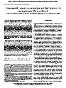
The Kentucky benchmark checks the retrieval of images associated with objects. To check whether our method properly identifies the location from which images were captured, we used a different test. We captured a topology in two environments — a design lab, built to mimic a real apartment, and the home of one of the authors. The two environments are sketched in Figure 2. In both environments we captured a topology consisting of 7 distinct locations and edges between adjacent locations.
4 3.9 3.8 3.7 3.6 3.5 3.4 3.3 3.2 3.1 3 0
2500
5000
50F 1S
50F 2S
100F 2S
Visual words
7500
10000 100F 1S
(a) Design lab sketch Figure 1: Performance of our image retrieval methods on the University of Kentucky benchmark. We plot the average number of images of the same object that were identified (4 at most), as the number of objects grow. In the experiment we evaluated both the rapid first stage only (denoted 1S), and the two stage method (denoted 2S) we use on our robot. We also compare the use of 50 features (denoted 50F) and 100 features (denoted 100F) for each image. We trained the signature weights using gradient descent over the first 1000 images, and then fixed the weights for the rest of the images. As we can see from Figure 1, our image comparison method provides better results, especially as the number of images grow, than the Visual Words of [17]3 . As expected, 2 stages provide better results, and more features help. Our method is also very fast, and queries take less than 1 microsecond (µs) for the first stage, and 200µs for the second stage, over a 1000 image dataset which 1
www.microsoft.com/robotics www.vis.uky.edu/\~stewe/ukbench/ 3 The results for the visual words approach were interpolated from the graph at www.vis.uky.edu/\~stewe/ukbench/ and are therefore inexact. 2
(b) Home sketch
Figure 2: Sketches of the environments used in the experiments. We then split the captured images into a train and test set, by moving every other image into a test set, learning a topology only for the remaining images. Then, for every image in the test set, we ran a query against the dataset. We computed how many times the most likely state for each test image — maxs pr(o|s) — was the location or edge where the image was captured, and compute the classification error rate (Table 1). While our results show a high classification accuracy, this experiment does not properly evaluate our complete approach, because in some cases even when the most likely state was incorrect, the second most likely state was correct with minor probability difference.
9.3
Navigation performance
While image retrieval and localization are both key components in our appearance based approach, we are interested in evaluating the complete approach to localization and navigation. To evaluate our approach, we ran experiments in the two environments. In both environments we have captured a topology and instructed the robot
afterwards to move from one location to another multiple times. Table 2 shows the success rate in the two environments. Overall, we ran 30 tests, with a success rate of 86%. As we can see, the performance in the design lab is optimal, while in the real home the robot failed to reach the destination in several cases. This is not surprising, because the design lab had perfect floor conditions, where the robot wheels never slip, while the home had varying floor texture — tiles, carpets, and wood — where the robot occasionally gets stuck or spins too fast. Also, the lab has no outside windows, and therefore has constant lighting conditions. The home experiment was conducted during a few days, with varying outside conditions (from sunny to cloudy) and therefore different lighting conditions. These experiment hint that our mechanical design is not yet perfect, and that we would need a better driving system, and that varying lighting conditions add a level of difficulty. We can handle different lighting conditions by adding signatures to each image that are indifferent to varying lighting.
Environment Design Lab Design Lab Design Lab Design Lab Design Lab Design Lab Design Lab Home Home Home
Table 2: Results of path execution. Path Trials Entry ⇒ Snack bar 3 Snack bar ⇒ Entry 3 Snack bar ⇒ Corner desk 2 Corner desk ⇒ Entry 2 Entry ⇒ Corner desk 2 Gray cabinets ⇒ Corner desk 3 Corner desk ⇒ Gray cabinets 2 Office ⇒ Entry 5 Office ⇒ Piano 4 Office ⇒ Entry ⇒ Piano 4
Success 3 3 2 2 2 3 2 4 2 3
As in this paper we only focus on reaching the goal, rather than optimality, we do not report here the time or the length of the traversed paths. We note, however, that in some cases the robot choose a non-optimal path to the goal, and in some cases got disoriented on the way and had to explore the current surrounding to re-localize itself.
10.
DISCUSSION AND FUTURE WORK
In our implementation we use a number of either ad-hoc or manually tuned parameters. This is because we are interested in a real application for a specific robot platform. An obvious next step is to allow for generalization by learning such parameters online. In practice, we would still need to begin with a reasonable model that may contain many manually tuned parameters. However, we can later learn to tune these parameters to achieve better performance. Below we illustrate a number of suggestions for such improvements that we intend to explore.
10.1
Learning transition probabilities
Currently, transition probabilities are manually tuned to fit the domains and robots we experimented with, as learning the probabilities from experience may require many trials, and we currently aim at a robot that can be deployed very rapidly. However, learning these probabilities from trials is a viable alternative that will be pursued in the future. An attractive hybrid approach would begin with the hand-tuned probabilities, and will refine them by learning from experience, optimizing the robot to the actual environment it was deployed in. Also, our graph compaction approach assumes that all components with identical relations behave similarly. This does not allow us to learn that some edges are harder to traverse
than others, perhaps due to difficult curves. It is possible, however, to learn relation-free transition probabilities. Again, such probabilities would require significantly more trials before converging to a reliable value.
10.2
Interactive learning of the environment
During the initial tour of the environment, it is possible that the robot will pass several times through the same location, requiring either that the human will explicitly specify that this is an existing location, as our current implementation requires, or that the robot will identify that it is passing through an existing location. The latter approach can be augmented by presenting question to the person. For example, when the robot computes a high probability that the current location was already visited it can ask the human “are we in the kitchen?”. Such questions can ensure that the captured topology is accurate.
10.3
Topology Refinement
While the topology that we currently capture, i.e. rooms and corridors, may be easy for humans to understand and teach, it may not be the best topology for navigation. For example, a human will not identify a junction of two corridors as an important location, but adding such a location can help the robot considerably during navigation. We could, however, use the captured paths to infer such junctions of paths. If two edges start at the same location, we can trace the similarity of the images, starting from the first image. If the two paths have similar prefixes, we can decide to unify these prefixes, causing a new location to be added to the graph where the two paths becomes distinct. We can apply this procedure iteratively until no new locations are found.
10.4
Learning new paths
As we intend the teaching phase to be minimal, we do not expect that every two locations will be connected by a path. However, we can later learn new paths to enrich the graph. We suggest a simple exploration heuristic, that starts at a given location, and moves towards the open spaces, while trying to move away from its origin. While executing this exploration heuristic, it is likely that we will eventually reach some known location. If we record the images that were observed during the exploration, we can insert a new path into the graph, from the origin location to the destination location. These paths are not expected to be optimal, but as our exploration heuristic tries to avoid loops, the paths obtained this way are in many cases reasonable.
10.5
Learning new locations
Learning new meaningful locations in the closed environment is less straight forward. First, in order for a location to be meaningful it has to be labeled so that the robot can be commanded to go there. Second, we assume that the human teacher will show the robot all places of interest - (not true - in the case of an office environment we would like the robot to learn all the offices without showing them explicitly).
11.
CONCLUSION
In this paper we have presented a complete approach to appearancebased localization and navigation. We aim at low cost robots that could be used by anyone, and therefore choose an infrastructure consisting only of low cost components, such as a web cam, a depth camera, and a standard computer. Even with our cheap machine architecture, we have demonstrated an image identification system
with high precision, and a navigation system that robustly reaches the destination. Instead of eliminating the uncertainty in localization, we use a partially observable Markov decision process to estimate the uncertainty, and leverage this model to provide robust localization and navigation. Our approach is yet imperfect, mainly requiring additional engineering for more robust driving mechanism, and additional work on improving the image retrieval mechanism, as well as other stages of our approach, such as the environment capturing phase. In our implementation we use a number of either ad-hoc or manually tuned parameters. This is because we are interested in a real application for a specific robot platform. An obvious next step is to allow for generalization by learning such parameters online. In practice, we would still need to begin with a reasonable model that may contain many manually tuned parameters. However, we can later learn to tune these parameters to achieve better performance. In the future we will explore such options for learning new paths and locations, learning the transition probabilities, and topology refinement. Still, our approach provides a robust localization and navigation engine that can be used on robots with standard, affordable, hardware.
12.
[11]
[12]
[13]
[14]
[15]
[16]
REFERENCES
[1] Ronen Basri, Ehud Rivlin, and Ilan Shimshoni. Visual homing: Surfing on the epipoles. Int. J. Comput. Vision, 33(2):117–137, 1999. [2] Aeron Buchanan and Andrew Fitzgibbon. Interactive feature tracking using k-d trees and dynamic programming. In Computer Vision and Pattern Recognition, IEEE Computer Society Conference on, pages 626–633, 2006. [3] Wolfram Burgard, Dieter Fox, Daniel Hennig, and Timo Schmidt. Estimating the absolute position of a mobile robot using position probability grids. In In Proceedings of the Thirteenth National Conference on Artificial Intelligence, Menlo Park, pages 896–901. AAAI, AAAI Press/MIT Press, 1996. [4] Mark Cummins and Paul Newman. FAB-MAP: Probabilistic Localization and Mapping in the Space of Appearance. The International Journal of Robotics Research, 27(6):647–665, 2008. [5] Frank Dellaert, Dieter Fox, Wolfram Burgard, and Sebastian Thrun. Monte carlo localization for mobile robots. In IEEE International Conference on Robotics and Automation (ICRA99), May 1999. [6] H. Durrant-Whyte and T. Bailey. Simultaneous localisation and mapping (slam): Part i the essential algorithms. Robotics and Automation Magazine, 13:99—110, 2006. [7] Amalia Foka and Panos Trahanias. Real-time hierarchical pomdps for autonomous robot navigation. In IJCAI Workshop Reasoning with Uncertainty in Robotics, 2005. [8] C. Harris and M. Stephens. A combined corner and edge detector. In Proc. Fourth Alvey Vision Conference, pages 147–151, May 1988. [9] Hongwen Kang, Alexei A. Efros, Martial Hebert, and Takeo Kanade. Image matching in large scale indoor environment. In IEEE Computer Society Conference on Computer Vision and Pattern Recognition (CVPR) Workshop on Egocentric Vision, June 2009. [10] David Kortenkamp and Terry Weymouth. Topological mapping for mobile robots using a combination of sonar and
[17]
[18]
[19]
[20]
[21]
[22]
[23]
[24]
[25]
[26]
vision sensing. In AAAI’94: Proceedings of the twelfth national conference on Artificial intelligence (vol. 2), pages 979–984, Menlo Park, CA, USA, 1994. American Association for Artificial Intelligence. Ben J. A. Kröse, Nikos A. Vlassis, Roland Bunschoten, and Yoichi Motomura. A probabilistic model for appearance-based robot localization. Image Vision Comput., 19(6):381–391, 2001. David G. Lowe. Distinctive image features from scale-invariant keypoints. International Journal of Computer Vision, 60(2):91–110, 2004. J. Matas, O. Chum, U. Martin, and T. Pajdla. Robust wide baseline stereo from maximally stable extremal regions. In Proceedings of the British Machine Vision Conference, pages 384–393, 2002. Y. Matsumoto, K. Sakai, M. Inaba, and H. Inoue. View-based approach to robot navigation. In Intelligent Robots and Systems IROS, pages 1702–1708, November 2000. Krystian Mikolajczyk and Cordelia Schmid. An affine invariant interest point detector. In Proc. European Conf. Computer Vision, pages 128–142. Springer Verlag, 2002. Monica N. Nicolescu and Maja J Mataric. Experience-based representation construction: Learning from human and robot teachers. In In Proc., IEEE/RSJ Intl. Conf. on Intelligent Robots and Systems, pages 740–745, 2001. D. Nistér and H. Stewénius. Scalable recognition with a vocabulary tree. In IEEE Conference on Computer Vision and Pattern Recognition (CVPR), volume 2, pages 2161–2168, June 2006. Aude Oliva and Antonio Torralba. Building the gist of a scene: the role of global image features in recognition. In Progress in Brain Research, page 2006, 2006. J. M. Porta, J. J. Verbeek, and B. J. A. Kröse. Active appearance-based robot localization using stereo vision. Auton. Robots, 18(1):59–80, 2005. Emilio Remolina and Benjamin Kuipers. Towards a general theory of topological maps. Artificial Intelligence, 152:47–104, 2002. Edward J. Sondik Richard D. Smallwood. The optimal control of partially observable markov processes over a finite horizon. OPERATIONS RESEARCH, 21(5):1071–1088, 1973. Edward Rosten, , Edward Rosten, and Tom Drummond. Fusing points and lines for high performance tracking. In Proceedings of the International Conference on Computer Vision, pages 1508–1515. Springer, 2005. Matthijs T. J. Spaan and Nikos Vlassis. A point-based POMDP algorithm for robot planning. In Proceedings of the IEEE International Conference on Robotics and Automation, pages 2399–2404, New Orleans, Louisiana, 2004. Georgios Theocharous, Khashayar Rohanimanesh, and Sridhar Mahadevan. Learning hierarchical partially observable markov decision process models for robot navigation. In ICRA, pages 511–516, 2001. Iwan Ulrich and Illah Nourbakhsh. Appearance-based place recognition for topological localization. In Proceedings of ICRA 2000, volume 2, pages 1023 – 1029, April 2000. Andrew D. Wilson. Depth-sensing video cameras for 3d tangible tabletop interaction. In Horizontal Interactive Human-Computer Systems, International Workshop on, pages 201–204, 2007.