www.nature.com/scientificreports
OPEN
Received: 1 February 2018 Accepted: 26 April 2018 Published: xx xx xxxx
Auto-FPFA: An Automated Microscope for Characterizing Genetically Encoded Biosensors Tuan A. Nguyen, Henry L. Puhl III , An K. Pham & Steven S. Vogel Genetically encoded biosensors function by linking structural change in a protein construct, typically tagged with one or more fluorescent proteins, to changes in a biological parameter of interest (such as calcium concentration, pH, phosphorylation-state, etc.). Typically, the structural change triggered by alterations in the bio-parameter is monitored as a change in either fluorescent intensity, or lifetime. Potentially, other photo-physical properties of fluorophores, such as fluorescence anisotropy, molecular brightness, concentration, and lateral and/or rotational diffusion could also be used. Furthermore, while it is likely that multiple photo-physical attributes of a biosensor might be altered as a function of the bio-parameter, standard measurements monitor only a single photo-physical trait. This limits how biosensors are designed, as well as the accuracy and interpretation of biosensor measurements. Here we describe the design and construction of an automated multimodal-microscope. This system can autonomously analyze 96 samples in a micro-titer dish and for each sample simultaneously measure intensity (photon count), fluorescence lifetime, time-resolved anisotropy, molecular brightness, lateral diffusion time, and concentration. We characterize the accuracy and precision of this instrument, and then demonstrate its utility by characterizing three types of genetically encoded calcium sensors as well as a negative control. Fluorescence microscopy has been extensively used as a tool for monitoring biological molecules of interest that can be tagged with a fluorophore1–3. With proper instrumentation, several aspects of fluorescence can be monitored4, including emission intensity, absorption spectrum, emission spectrum, lifetime, anisotropy, concentration, molecular brightness, and the lateral & rotational diffusion of the fluorophore. The discovery of genetically encoded Green Fluorescent Protein (GFP)5 and the rapid development and bioengineering of genetic variants of GFP6–9 and related proteins (FPs) has led to the development of genetically encoded biosensors that typically have one or more FPs attached to a protein moiety designed to change its structural conformation in response to a biological parameter of interest, such as free calcium10. By diligent and creative genetic engineering, bio-parameter induced structural changes will alter the photo-physics of attached fluorophores, and these changes in the photo-physics can be monitored with appropriate instrumentation to estimate changes in the bio-parameter of interest. Unfortunately, the majority of biosensors currently available work by detecting only changes in the intensity of one or more fluorophores, while information imbedded in the other modes of fluorescence have remained unexplored and untapped. We believe that this limitation on the design pallet available to biosensor developers arises primarily because of a lack of instrumentation that can 1: rapidly & reliably, and 2: simultaneously measure multiple photo-physical changes in biosensors. Automated microscopes11–15 have been developed to address the first issue, but robotic systems that can concurrently monitor multiple photo-physical properties have not been reported. In this paper, we describe the design, construction, and utility of an automated multi-modal microscope that simultaneously measures fluorescence intensity (photon count), lifetime, time-resolved anisotropy, molecular brightness, concentration, and lateral diffusion.
Results
Design and implementation of Auto-Fluorescence Polarization and Fluctuation Analysis (autoFPFA). We previously designed a microscope that used two-photon linearly polarized pulsed excitation in conjunction with time-correlated single photon counting (TCSPC) instrumentation to measure fluctuations in
Laboratory of Molecular Physiology, National Institute on Alcohol Abuse and Alcoholism, National Institutes of Health, 5625 Fishers Lane, Rockville, Maryland, USA. Correspondence and requests for materials should be addressed to S.S.V. (email:
[email protected]) ScIeNtIfIc REPOrTS | (2018) 8:7374 | DOI:10.1038/s41598-018-25689-x
1
www.nature.com/scientificreports/
Figure 1. Auto-FPFA schematic. The light path and components used for implementing auto-FPFA. Key components that have been added or modified from previous implementations of FPFA include the integration of a XY-dual axis scanning stage controller, a Z-axis stage controller, and the use of a 0.9 NA 40x air objective.
the intensity of parallel, I||(t), and perpendicular, I⊥ (t), polarized fluorescent emissions over time, as well as the fluorescence intensity decay of the parallel, I||(∆t), and perpendicular I⊥ (∆t), polarization, as a function of time after an excitation laser pulse16–19. I||(t), and I⊥ (t) were cross correlated for fluorescence correlation spectroscopy (FCS) analysis to reveal bio-photonic attributes of a sample such as count-rate, molecular brightness, concentration, and τD20–22. I||(∆t), and I⊥ (∆t) are used to calculate the fluorescence lifetime decay of the sample as well as its time-resolved anisotropy decay11,23–26. We called this multimodal approach Fluorescence Polarization and Fluctuation Analysis (FPFA)16. In this paper, we set out to design an automated variant of FPFA to autonomously measure up to 96 samples. The major design challenges for implementing FPFA microscopy is that FCS microscopy signal to noise is optimized by using high numerical aperture (NA) objectives that minimize the excitation volume27–32. In contrast, time resolved anisotropy measurements are best implemented using low NA objectives to minimize depolarization33,34. Furthermore, to build an automated variant of FPFA for micro-titer plates it is advantageous to avoid objectives that require oil or water deposition between the objective and the bottom of the plate as liquids can evaporate, drip or enclose bubbles that can corrupt automated measurements. Finally, for accurate FCS measurements the excitation volume of an objective, as defined by its point spread function35, should reside completely within the sample volume. Thus, objectives with long working distance are advantageous, in conjunction with an automated focus mechanism to keep the excitation volume well within the sample volume as an automated X-Y stage moves systematically through all samples. The design of our implementation of auto-FPFA is illustrated in Fig. 1. An 80 MHz, 70-fs Ti:Sapphire laser (MaiTai eHP, Spectra-Physics) tuned to 950 nm is used for two-photon excitation. The laser is filtered and expanded (KT310, Thorlabs), and then passed through a laser attenuator consisting of near-IR half-wave plate and linear polarizer (100,000:1 extinction ratio, Thorlabs) where the excitation power and polarization at the sample can be adjusted. Next, the excitation beam is directed through a multiphoton long-pass dichroic beamsplitter (FF665-Di02-25 × 36, Semrock) to an air microscope objective (Zeiss 40x 0.9 NA, with back aperture slightly overfilled) that focuses the beam to a diffraction-limited spot (~0.5 μm in diameter) to form the excitation/observation volume (1.7 ± 0.7 fl). Sample fluorescence emanating from the observation volume was reflected by the same dichroic beam-splitter and then filtered by a high throughput two-photon band-pass emission filter (FF01520/70-25, Semrock). The fluorescence emission is next guided to a polarizing beam splitter augmented with two orthogonally oriented linear polarizers (Thorlabs) to increase the polarization extinction ratio. At the polarizing beam splitter, parallel and perpendicular emitted photons are separated and each signal is detected by its own dedicated HPM-100-40 hybrid detector (Becker & Hickl). The dark count rate for these detectors is 300–600 cps at room temperature. Detected photons were passed to a SPC-130 EM TCSPC card (Becker & Hickl) via a router (HRT-41, Becker and Hickl). For synchronization with excitation pulses a small fraction of the excitation beam was focused onto a fast photodiode (DET10N, Thorlabs). The SPC-130 card records both micro-time (the time between excitation and photon detection) and macro-time (the time between experiment initiation and photon detection) for each parallel and perpendicular photon detected. Samples are pipetted into a glass-bottom 96-well microplate (Greiner Bio-One). The plate is then attached onto a XY motorized stage (HLD117, Prior Scientific) so that samples can be scanned over the microscope objective. To compensate for imperfections in the flatness of these microplates, a system was created to automatically ScIeNtIfIc REPOrTS | (2018) 8:7374 | DOI:10.1038/s41598-018-25689-x
2
www.nature.com/scientificreports/
Figure 2. Auto-FPFA acquisition software control and software/hardware interface schematic. Left Panel: Diagram illustrates the Lab View control algorithm, and its integration with B&H SPCM software algorithm. LabView was used as the ‘master’ control data acquisition software, while B&H SPCM software was ‘slaved’ to it. LabView specifically controlled the XY-dual axis scanning stage controller that sequentially steps through the 96 samples in a micro-titer dish, as well as the Z-axis stage controller used for the auto-focus function. The ‘slaved’ B&H SPCM software was used to control the TCSPC SPC-130-EM card for data acquisition and data storage. Right Panel: Diagram illustrates the auto-FPFA software/hardware interface. The central component of this system is the B&H SPC 130-EM TCSPC card. Both LabView and B&H SPCM software communicate (send commands and receive data) with the TCSPC card via a B&H SPC driver. Once activated, the TCSPC card receives data from the two HPM-100-40 hybrid photon detectors via a HRT 41 multiplexing router. The TCSPC card also receives laser pulse timing data from a photo-diode detector (not shown, but see Fig. 1).
focus along the Z-axis at each well location. This was implemented by inversely mounting the objective on a post-mountable focus block (MGZ30, Thorlabs) whose fine adjustment knob was attached to a motorized microscope focus controller (MFC1, Thorlabs) to provide computerized Z axis adjustments. SPCM software (Becker & Hickl, Ver. 9.6) running in FIFO mode was used for data acquisition, storage and calculation of time-resolved fluorescence and auto-/cross-correlation functions from micro- and macro-time data, respectively. In parallel, X-Y and Z motorized stages were controlled via a custom LabView (National Instruments, Ver. 2015) program based on the manufacture’s libraries. The coordination between LabView and SCPM software for Auto-FPFA, as well as the software-hardware interface is displayed in Fig. 2. Prior to initializing an experiment, it is important to perform system calibration, laser power adjustment, background and sample trial measurements (so that the sample’s concentration can be optimized) and the software parameters for both LabView and SPCM software entered into each program. Next, the TCSPC card is primed and put into TTL-triggered waiting mode. To initiate an auto-FPFA experiment the LabView software is started. This moves the microplate so that the first (next) sample is positioned above the objective. Next, the auto-focus sub-routine is launched. The Z-axis controller systematically moves the objective up toward the sample. At each Z-axis location, the fluorescent intensity is recorded and compared to previous measurements to find the Z-axis position that has the maximum fluorescence intensity. Once the optimal Z-axis position is found, a TTL signal is sent by LabView to trigger data acquisition on the TCSPC card. The LabView software enters a waiting period set to be equal to the photon collection time parameter of the TCSPC card, plus an additional 20 seconds so that the SPCM card has sufficient time to acquire and save the data and prime TCSPC card for the next sample well acquisition. This cycle is repeated until all sample wells are scanned. Two-photon excitation power (at the sample) was typically 9.6 mW to avoid bleaching during acquisition (~150–200 s per well)., Motorized stage components were anchored via Ø1.5” damped posts (Thorlabs) to minimized mechanical vibrations. For each sample, averaged measurements were acquired from three to five repeats. All experiments were performed at room temperature.
ScIeNtIfIc REPOrTS | (2018) 8:7374 | DOI:10.1038/s41598-018-25689-x
3
www.nature.com/scientificreports/
Figure 3. Auto-FPFA accuracy and reproducibility. Auto-FPFA measurements of the molecular brightness (a), diffusion time (τD, b), steady state anisotropy (c), and lifetime (d) of Venus monomers. Four cell homogenates (circle, square, triangle and diamond symbols) were prepared from cells expressing the Venus fluorescent protein. Replicates of these homogenates were deposited in 24 different wells of a micro-titer dish and all 96wells were measured overnight by auto-FPFA. Red bars indicate the mean of the 24 replicates of each sample. Note the outlier that is easily detected in Venus sample #3 in panel d.
The accuracy & precision of auto-FPFA. To characterize the accuracy and precision of auto-FPFA we
prepared four homogenates from cells transfected with a DNA construct to express the fluorescent protein mVenus36. For each, 24 200 µl replicates were pipetted into wells of a microtiter-dish (making a total of 96 wells) and automated data acquisition was initiated. For each well three 200 s data acquisition periods were acquired and results were averaged. Thus, each well took ~10 minutes for data acquisition and the whole plate required ~16 hours. Because each well of the microtiter dish had mVenus, we used this experiment to characterize the repeatability of our measurements. The molecular brightness for the mVenus replicates are depicted in Fig. 3a and had values of: 863 ± 74, 849 ± 64, 809 ± 72, and 852 ± 61 cpms (mean ± SD, n = 24), and the ensemble mean was 843 ± 70 cpms (mean ± SD, n = 96). A brightness of 843 cpms should have a Poisson counting error of ~29 counts. Thus, the additional error we measure (41 counts) represents 5% of our total mVenus brightness. Diffusion time (τD) measurements are depicted in Fig. 3b and had values of: 377 ± 58, 382 ± 71, 405 ± 73, and 372 ± 50 µs (mean ± SD, n = 24) and the ensemble τD value was 383 ± 61 µs (mean ± SD, n = 96). Our error represents ~16% of our total τD. The steady-state anisotropy for the mVenus replicates are depicted in Fig. 3c and had values of: 0.419 ± 0.001, 0.420 ± 0.001, 0.420 ± 0.002, and 0.420 ± 0.001(mean ± SD, n = 24) and the ensemble anisotropy value was 0.420 ± 0.002 (mean ± SD, n = 96). Our error represents approximately 0.5% of our signal. The mVenus fluorescence lifetime for the four replicate groups are depicted in Fig. 3d and had values of: 3.154 ± 0.005, 3.156 ± 0.005, 3.137 ± 0.090, and 3.155 ± 0.005 ns (mean ± SD, n = 24) and the ensemble lifetime value was 3.150 ± 0.045 ns (mean ± SD, n = 96). Note that one well from group #3 appeared to be an outlier (panel 3d), and was confirmed by a failure in a D’Agostino & Pearson normality test for group #3 (P