Automatic Abstraction Using Generalized Model Checking Patrice Godefroid1 and Radha Jagadeesan⋆2 1
2
Bell Laboratories, Lucent Technologies,
[email protected] Department of Computer Science, Loyola University of Chicago,
[email protected]
Abstract. Generalized model checking is a framework for reasoning about partial state spaces of concurrent reactive systems. The state space of a system is only “partial” (partially known) when a full state-space exploration is not computationally tractable, or when abstraction techniques are used to simplify the system’s representation. In the context of automatic abstraction, generalized model checking means checking whether there exists a concretization of an abstraction that satisfies a temporal logic formula. In this paper, we show how generalized model checking can extend existing automatic abstraction techniques (such as predicate abstraction) for model checking concurrent/reactive programs and yield the three following improvements: (1) any temporal logic formula can be checked (not just universal properties as with traditional conservative abstractions), (2) correctness proofs and counter-examples are both guaranteed to be sound, and (3) verification results can be more precise. We study the cost needed to improve precision by presenting new upper and lower bounds for the complexity of generalized model checking in the size of the abstraction.
1
Introduction
How to broaden the scope of model checking to reactive software is currently one of the most challenging open problems related to computer-aided verification. Essentially two approaches have been proposed and are still actively being investigated. The first approach consists of adapting model checking into a form of systematic testing that simulates the effect of model checking while being applicable to (Unix-like) processes executing arbitrary code [10]; although counterexamples reported with this approach are sound, it is inherently incomplete for large systems. The second approach consists of automatically extracting a model out of a software application by statically analyzing its code, and then of analyzing this model using traditional model-checking algorithms (e.g., [2, 6, 25, 21, 14]); although automatic abstraction may be able to prove correctness, counterexamples are generally unsound since abstraction usually introduces unrealistic behaviors that may yield to spurious errors being reported when analyzing the model. ⋆
Supported in part by NSF.
Recently [11], we showed how automatic abstraction can be performed to verify arbitrary formulas of the propositional µ-calculus [17] in such a way that both correctness proofs and counter-examples are guaranteed to be sound. The key to make this possible is to represent abstract systems using richer models that distinguish properties that are true, false and unknown of the concrete system. Examples of such richer modeling formalisms are partial Kripke structures [3] and Modal Transition Systems [19, 11]. Reasoning about such systems requires 3-valued temporal logics [3], i.e., temporal logics whose formulas may evaluate to true, false or ⊥ (“unknown”) on a given model. Then, by using an automatic abstraction process that generates by construction an abstract model which is less complete than the concrete system with respect to a completeness preorder logically characterized by 3-valued temporal logic, every temporal property that evaluates to true (resp. false) on the abstract model automatically holds (resp. does not hold) of the concrete system, hence guaranteeing soundness of both proofs and counter-examples; in case a property evaluates to ⊥ on the model, a more complete (i.e., less abstract) model is then necessary to provide a definite answer concerning this property of the concrete system. This approach is applicable to check arbitrary formulas of the propositional µ-calculus (thus including negation and arbitrarily nested path quantifiers), not just universal properties as with a traditional “conservative” abstraction that merely simulates the concrete system. It is shown in [11] that building a 3-valued abstraction can be done using existing abstraction techniques at the same computational cost as building a conservative abstraction. In this paper, we build upon this previous work and study the use of generalized model checking in the context of automatic abstraction. Generalized model checking was introduced in [4] as a way to improve precision when reasoning about partially defined systems. Specifically, given a model M and a temporallogic formula φ, the generalized model-checking problem is to decide whether there exists a complete system M ′ that is more complete than M and that satisfies the formula φ. The model M can thus be viewed as a partial solution to the satisfiability problem for φ which reduces the solution space to complete systems that are more complete than M with respect to a completeness preorder. Generalized model checking is thus a generalization of both satisfiability and model checking. Algorithms and complexity bounds for the generalized model-checking problem for various temporal logics were presented in [4]. We present here several new results. First, we study the complexity of generalized model checking in the size of the abstraction |M |, and provide new upper and lower bounds for various temporal logics. We show that the worst-case runtime complexity of generalized model checking for the temporal logics LTL and CTL can be quadratic in |M |, but that generalized model checking can be solved in time linear in |M | in the case of persistence properties, i.e., properties recognizable by co-B¨ uchi automata. Complexity in the size of the abstraction is important in practice since the abstraction can be large and hence is often the main limiting factor that prevents obtaining verification results.
Second, we show how generalized model checking can help improve precision of verification via automatic abstraction. We present a new process for iterative abstraction refinement that takes advantage of the techniques introduced here. Iterative abstraction refinement [1, 9, 13] in the context of predicate abstraction [12] is a process for automatically refining an abstraction that is guided by spurious counter-examples found at higher levels of abstraction. In contrast with abstractions used in traditional program analysis, iterative abstraction refinement using predicate abstraction has thus the advantage of making it possible to adapt the level of abstraction dynamically on a demand-driven basis guided by the verification needs. Unfortunately, refining an abstraction can be an expensive operation since successive abstraction refinements can generate exponentially larger abstractions. Better precision when analyzing an abstraction is therefore critical to avoid unnecessary refinements of this abstraction. We believe generalized model checking is a useful addition to existing techniques for automatic abstraction since it can help an iterative “abstract-check-refine” verification process terminate sooner and more often by providing better analysis precision for a cost polynomial (quadratic or linear) in the size of the abstraction.
2
Background: Generalized Model Checking
In this section, we recall the main ideas and key notions behind the framework of [3, 4, 11, 15] for reasoning about partially defined systems. Examples of modeling formalisms for representing such systems are partial Kripke structures (PKS) [3], Modal Transition Systems (MTS) [19, 11] or Kripke Modal Transition Systems (KMTS) [15]. must may
Definition 1. A KMTS M is a tuple (S, P, −→ , −→, L), where S is a nonempty may must finite set of states, P is a finite set of atomic propositions, −→⊆ S ×S and −→ ⊆ must may S × S are transition relations such that −→ ⊆−→, and L : S × P → {true, ⊥ , false} is an interpretation that associates a truth value in {true, ⊥, false} with each atomic proposition in P for each state in S. An MTS is a KMTS where must may P = ∅. A PKS is a KMTS where −→ =−→. The third value ⊥ (read “unknown”) and may-transitions that are not musttransitions are used to model explicitly a loss of information due to abstraction concerning, respectively, state or transition properties of the concrete system being modeled. A standard, complete Kripke structure is a special case of KMTS must may where −→ =−→ and L : S × P → {true, false}, i.e., no proposition takes value ⊥ in any state. It can be shown that PKSs, MTSs, KMTSs and variants of KMTSs where transitions are labeled and/or two interpretation functions Lmay and Lmust are used [15], are all equally expressive (i.e., one can translate any formalism into any other). In this paper, we will use KMTSs since they conveniently generalize models with may-transitions only, which are used with traditional conservative abstractions. Obviously, our results also hold for other equivalent formalisms (exactly as traditional model-checking algorithms and complexity
bounds apply equally to systems modeled as Kripke structures or Labeled Transition Systems, for instance). In interpreting propositional operators on KMTSs, we use Kleene’s strong 3-valued propositional logic [16]. Conjunction ∧ in this logic is defined as the function that returns true if both of its arguments are true, false if either argument is false, and ⊥ otherwise. We define negation ¬ using the function ‘comp’ that maps true to false, false to true, and ⊥ to ⊥. Disjunction ∨ is defined as usual using De Morgan’s laws: p ∨ q = ¬(¬p ∧ ¬q). Note that these functions give the usual meaning of the propositional operators when applied to values true and false. Propositional modal logic (PML) is propositional logic extended with the modal operator AX (which is read “for all immediate successors”). Formulas of PML have the following abstract syntax: φ ::= p | ¬φ | φ1 ∧ φ2 | AXφ, where p ranges over P . The following 3-valued semantics generalizes the traditional 2-valued semantics for PML. Definition 2. The value of a formula φ of 3-valued PML in a state s of a KMTS must may M = (S, P, −→ , −→, L), written [(M, s) |= φ], is defined inductively as follows: [(M, s) |= p] = L(s, p) [(M, s) |= ¬φ] = comp([(M, s) |= φ]) [(M, s) |= φ1 ∧ φ2 ] = [(M, s) |= φ1 ] ∧ [(M, s) |= φ2 ] may true if ∀s′ : s −→ s′ ⇒ [(M, s′ ) |= φ] = true must [(M, s) |= AXφ] = false if ∃s′ : s −→ s′ ∧ [(M, s′ ) |= φ] = false ⊥ otherwise
This 3-valued logic can be used to define a preorder on KMTSs that reflects their degree of completeness. Let ≤ be the information ordering on truth values, in which ⊥ ≤ true, ⊥ ≤ false, x ≤ x (for all x ∈ {true, ⊥, false}), and x 6≤ y otherwise. must
may
must
Definition 3. Let MA = (SA , P, −→ A , −→A , LA ) and MC = (SC , P, −→ C may , −→C , LC ) be KMTSs. The completeness preorder ¹ is the greatest relation B ⊆ SA × SC such that (sa , sc ) ∈ B implies the following: – ∀p ∈ P : LA (sa , p) ≤ LC (sc , p), must must – if sa −→ A s′a , there is some s′c ∈ SC such that sc −→ C s′c and (s′a , s′c ) ∈ B, may may – if sc −→C s′c , there is some s′a ∈ SA such that sa −→A s′a and (s′a , s′c ) ∈ B. This definition allows to abstract MC by MA by letting truth values of propositions become ⊥ and by letting must-transitions become may-transitions, but all may-transitions of MC must be preserved in MA . We then say that MA is more abstract, or less complete, than MC . The inverse of the completeness preorder is also called refinement preorder in [19, 15, 11]. Note that relation B reduces to a simulation relation when applied to MTSs with may-transitions only. It can be shown that 3-valued PML logically characterizes the completeness preorder [3, 15, 11].
must
may
must
may
Theorem 1. Let MA = (SA , P, −→ A , −→A , LA ) and MC = (SC , P, −→ C , −→C , LC ) be KMTSs such that sa ∈ SA and sc ∈ SC , and let Φ be the set of all formulas of 3-valued PML. Then, sa ¹ sc iff (∀φ ∈ Φ : [(MA , sa ) |= φ] ≤ [(MC , sc ) |= φ]). In other words, KMTSs that are “more complete” with respect to ¹ have more definite properties with respect to ≤, i.e., have more properties that are either true or false. Moreover, any formula φ of 3-valued PML that evaluates to true or false on a KMTS has the same truth value when evaluated on any more complete structure. This result also holds for PML extended with fixpoint operators, i.e., the propositional µ-calculus [3]. In [11], we showed how to adapt the abstraction mappings of [8] to construct abstractions that are less complete than a given concrete program with respect to the completeness preorder. must
may
Definition 4. Let MC = (SC , P, −→ C , −→C , LC ) be a (concrete) KMTS. Given a set SA of abstract states and a total3 abstraction relation on states ρ ⊆ SC ×SA , may must we define the (abstract) KMTS MA = (SA , P, −→ A , −→A , LA ) as follows: must
must
– a −→ A a′ if ∀c ∈ SC : cρa ⇒ (∃c′ ∈ SC : c′ ρa′ ∧ c −→ C c′ ); may may – a −→A a′ if∃c, c′ ∈ SC : cρa ∧ c′ ρa′ ∧ c −→C c′ ; true if ∀c : cρa ⇒ LC (c, p) = true – LA (a, p) = false if ∀c : cρa ⇒ LC (c, p) = false ⊥ otherwise
The previous definition can be used to build abstract KMTSs.
Theorem 2. Given a KMTS MC , any KMTS MA obtained by applying Definition 4 is such that MA ¹ MC . Given a KMTS MC , any abstraction MA less complete than MC with respect to the completeness preorder ¹ can be constructed using Definition 4 by choosing the inverse of ρ as B [11]. When applied to MTSs with may-transitions only, the above definition coincides with traditional “conservative” abstraction. Building a 3-valued abstraction can be done using existing abstraction techniques at the same computational cost as building a conservative abstraction [11]. Since by construction MA ¹ MC , any temporal-logic formula φ that evaluates to true (resp. false) on MA automatically holds (resp. does not hold) on MC . It is shown in [4] that computing [(MA , s) |= φ] can be reduced to two traditional (2-valued) model-checking problems on regular fully-defined systems (such as Kripke structures or Labeled Transition Systems), and hence that 3valued model-checking for any temporal logic L has the same time and space complexity as 2-valued model checking for the logic L. However, as argued in [4], the semantics of [(M, s) |= φ] returns ⊥ more often than it should. Consider a KMTS M consisting of a single state s such that the 3
That is, (∀c ∈ SC : ∃a ∈ SA : cρa) and (∀a ∈ SA : ∃c ∈ SC : cρa).
value of proposition p at s is ⊥ and the value of q at s is true. The formulas p ∨ ¬p and q ∧ (p ∨ ¬p) are ⊥ at s, although in all complete Kripke structures more complete than (M, s) both formulas evaluate to true. This problem is not confined to formulas containing subformulas that are tautological or unsatisfiable. Consider a KMTS M ′ with two states s0 and s1 such that p = q = true in s0 and p = q = false in s1 , and with a may-transition from s0 to s1 . The formula AXp ∧ ¬AXq (which is neither a tautology nor unsatisfiable) is ⊥ at s0 , yet in all complete structures more complete than (M ′ , s0 ) the formula is false. This observation is used in [4] to define an alternative 3-valued semantics for modal logics called the thorough semantics since it does more than the other semantics to discover whether enough information is present in a KMTS to give a definite answer. Let the completions C(M, s) of a state s of a KMTS M be the set of all states s′ of complete Kripke structures M ′ such that s ¹ s′ . Definition 5. Let φ be a formula of any two-valued logic for which a satisfaction relation |= is defined on complete Kripke structures. The truth value of φ in a state s of a KMTS M under the thorough interpretation, written [(M, s) |= φ]t , is defined as follows: true if (M ′ , s′ ) |= φ for all (M ′ , s′ ) in C(M, s) [(M, s) |= φ]t = false if (M ′ , s′ ) 6|= φ for all (M ′ , s′ ) in C(M, s) ⊥ otherwise
It is easy to see that, by definition, we always have [(M, s) |= φ] ≤ [(M, s) |= φ]t . In general, interpreting a formula according to the thorough three-valued semantics is equivalent to solving two instances of the generalized model-checking problem [4].
Definition 6 (Generalized Model-Checking Problem). Given a state s of a KMTS M and a formula φ of a (two-valued) temporal logic L, does there exist a state s′ of a complete Kripke structure M ′ such that s ¹ s′ and (M ′ , s′ ) |= φ ? This problem is called generalized model-checking since it generalizes both model must checking and satisfiability checking. At one extreme, where M = ({s0 }, P, −→ = may −→= {(s0 , s0 )}, L) with L(s0 , p) =⊥ for all p ∈ P , all complete Kripke structures are more complete than M and the problem reduces to the satisfiability problem. At the other extreme, where M is complete, only a single structure needs to be checked and the problem reduces to model checking. Algorithms and complexity bounds for the generalized model-checking problem for various temporal logics were presented in [4]. In the case of branchingtime temporal logics, generalized model checking has the same complexity in the size of the formula as satisfiability. In the case of linear-time temporal logic, generalized model checking is EXPTIME-complete in the size of the formula, i.e., harder than both satisfiability and model checking, which are both PSPACEcomplete in the size of the formula for LTL. Figure 1 summarizes the complexity results of [4]. These results show that the complexity in the size of the formula of computing [(M, s) |= φ]t (GMC) is always higher than that of computing [(M, s) |= φ] (MC).
Logic MC Propositional Logic Linear PML Linear CTL Linear µ-calculus NP∩co-NP LTL PSPACE-complete
SAT NP-complete PSPACE-complete EXPTIME-complete EXPTIME-complete PSPACE-complete
GMC NP-complete PSPACE-complete EXPTIME-complete EXPTIME-complete EXPTIME-complete
Fig. 1. Known results on the complexity in the size of the formula for (2-valued and 3-valued) model checking (MC), satisfiability (SAT) and generalized model checking (GMC).
Regarding the complexity in the size of the model |M |, it is only shown in [4] that generalized model checking can be solved in time quadratic in |M |. In the next two sections, we refine this result by presenting new upper and lower bounds for the complexity of generalized model checking in the size of the model for various classes of temporal properties. Our algorithms and constructions make use of automata-theoretic techniques (e.g., see [18]). For basic notions of automata theory (including definitions of nondeterministic/alternating/weak B¨ uchi automata on words and trees), please refer to [18]. Let us simply recall that a co-B¨ uchi acceptance condition is the dual of a B¨ uchi acceptance condition: an infinite execution w satisfies a co-B¨ uchi acceptance condition F if it does not intersect the set F of (rejecting) states infinitely often (i.e., Inf (w) ∩ F = ∅), while an infinite execution w satisfies a B¨ uchi acceptance condition F if it intersects the set F of (accepting) states infinitely often (i.e., Inf (w) ∩ F 6= ∅).
3
Generalized Model Checking for LTL
We first consider the case of properties expressed as linear-time temporal-logic (LTL) formulas [20]. To begin, we recall the following property of LTL: if φ is an LTL formula and (M, s) is a complete Kripke structure, (M, s) 6|= φ is not logically equivalent to (M, s) |= ¬φ. Indeed, if L(M, s) denotes the language of ω-words represented by (M, s), the former statement is equivalent to ∃w ∈ L(M, s) : w 6|= φ while the latter is equivalent to ∀w ∈ L(M, s) : w |= ¬φ, which in turn is equivalent to ∀w ∈ L(M, s) : w 6|= φ. Therefore, computing [(M, s) |= φ]t in the LTL case reduces to only one generalized model-checking problem, namely “does there exists a completion (M ′ , s′ ) of (M, s) such that (M ′ , s′ ) |= φ?”, plus a second problem of the form “does there exists a completion (M ′ , s′ ) of (M, s) such that (M ′ , s′ ) 6|= φ?”. This second problem is easier to solve than generalized model checking. Theorem 3. Given a state s of a KMTS M and a LTL formula φ, checking whether there exists a state s′ of a complete Kripke structure M ′ such that s ¹ s′ and (M ′ , s′ ) 6|= φ can be done in time linear in |M | and is PSPACE-complete in |φ|. Proof. (Sketch)4 For any two infinite sequences w = a1 a2 . . . and w′ = a′1 a′2 . . ., let w ≤ w′ denote that ∀i > 0 : ∀p ∈ P : L(ai , p) ≤ L(a′i , p). It is easy to show that 4
Complete proofs are omitted in this extended abstract due to space limitations.
∃(M ′ , s′ ) : s ¹ s′ ∧ (M ′ , s′ ) 6|= φ iff ∃w ∈ L(M, s) : ∃w′ : w ≤ w′ ∧ w′ 6|= φ. The latter condition can be reduced to checking nonemptiness of a nondeterministic B¨ uchi word automaton A defined by a product construction of the KMTS (M, s) and of a nondeterministic B¨ uchi automaton A¬φ accepting the set of ω-words violating the property φ. This product construction does not distinguish may and must transitions of M and attempts to match all of these to transitions of A¬φ ; occurrences of value ⊥ in M are matched to both values true and false in A¬φ ; the size of A is therefore linear in |M |. Checking nonemptiness of the resulting B¨ uchi automaton A can be done in time linear in |A| (hence linear in |M |). By analogy with traditional model checking, it is easy to show that the problem is also PSPACE-complete in |φ|.
Computing [(M, s) |= φ]t for an LTL formula φ can thus be done using the following procedure: 1. Check whether (M, s) × A¬φ = ∅. By the previous theorem, this can be done in time linear in |M | and is PSPACE-complete in |φ|. If the outcome of this check is positive (i.e., the product is empty), then all completions of (M, s) satisfy φ, and [(M, s) |= φ]t = true; otherwise, continue. 2. Check whether ∃(M ′ , s′ ) : s ¹ s′ ∧(M ′ , s′ ) |= φ (generalized model checking). As recalled in the previous section, this can be done in time quadratic in |M | and is EXPTIME-complete in |φ|. (Intuitively, this check is more expensive since it requires checking that ∀w ∈ L(M, s) : ∃w′ : w ≤ w′ ∧ w′ |= φ, which includes an alternation of ∀ and ∃.) If the outcome of this check is positive, we have [(M, s) |= φ]t =⊥; otherwise, all completions of (M, s) violate φ, and [(M, s) |= φ]t = false. Because Step 2 of the above procedure requires solving an instance of the generalized model-checking problem, the time needed to compute [(M, s) |= φ]t using the generalized model-checking algorithm of [4] can be quadratic in |M |. Unfortunately, the lower bound provided by the following theorem shows that it is unlikely this quadratic complexity can be reduced in the general case. Theorem 4. The problem of checking emptiness of nondeterministic B¨ uchi tree automata is reducible in linear time and logarithmic space to the generalized model-checking problem for LTL properties represented by nondeterministic B¨ uchi word automata. Since the worst-case run-time complexity of the best known algorithm for checking emptiness of nondeterministic B¨ uchi tree automata is quadratic in the size of the automaton [24], it is therefore unlikely that the generalized model-checking problem for LTL can be solved using better than quadratic time in |M | in the worst case. However, we now identify an important class of LTL formulas for which the generalized model-checking problem can be solved in time linear in |M |. This class is the class of persistence properties [20]. Persistence properties can be represented by LTL formulas of the form 3 2 p (where 3 is read “eventually” and 2 is read “always” [20]). Persistence properties also correspond to languages of ω-words recognizable by co-B¨ uchi automata.
Theorem 5. The generalized model-checking problem for LTL persistence properties can be solved in time linear in the size of the model. Proof. (Sketch) Every persistence property can be represented by a co-B¨uchi automaton Aφ . Aφ can then easily be transformed into a weak (B¨ uchi or co-B¨ uchi) nondeterministic automaton A′φ accepting the same language and of size linear in |Aφ |. Generalized model checking can then be reduced to checking emptiness of an alternating B¨ uchi word automaton A(M,s0 ),φ over a 1-letter alphabet defined using a product construction of the KMTS (M, s0 ) and the weak B¨ uchi automaton A′φ . If A′φ is weak, A(M,s0 ),φ is also weak. Moreover, the size of A(M,s0 ),φ is linear in |M |. Since checking emptiness of a weak alternating B¨ uchi word automaton over a 1-letter alphabet can be done in linear time [18], we obtain a decision procedure for the generalized model-checking problem of LTL persistence properties that is linear in |M |.
Of practical interest, persistence properties include all safety properties (LTL formulas of the form 2 p), as well as guarantee properties (LTL formulas of the form 3 p) and obligation properties (boolean combinations of safety and guarantee properties) [20]. Examples of LTL properties that are not persistence properties are response properties (LTL formulas of the form 2 3 p).
4
Generalized Model Checking for BTL
We now consider the case of branching-time temporal logics (BTL) such as propositional modal logic (e.g., see [23]), CTL [5] or the propositional µ-calculus [17]. In the case of a BTL formula φ, computing [(M, s) |= φ]t reduces to two generalized model-checking problems, namely “does there exist two completions (M ′ , s′ ) and (M ′′ , s′′ ) of (M, s) such that (M ′ , s′ ) |= φ and (M ′′ , s′′ ) 6|= φ?”, the latter statement being equivalent to (M ′′ , s′′ ) |= ¬φ. Given a CTL formula φ, the worst-case run-time complexity of computing [(M, s) |= φ]t for a CTL formula φ using the generalized model-checking algorithm of [4] is quadratic in |M |. The next theorem provides a lower bound similar to the one given in Theorem 4 in the LTL case. Theorem 6. The problem of checking emptiness of nondeterministic B¨ uchi tree automata is reducible in linear time and logarithmic space to the generalized model-checking problem for CTL properties represented by nondeterministic B¨ uchi tree automata. As in the LTL case, we can identify classes of properties for which generalized model checking can be done in time linear in |M |. Theorem 7. The generalized model-checking problem for BTL properties recognizable by nondeterministic co-B¨ uchi tree automata can be solved in time linear in the size of the model. Proof. (Sketch) BTL properties recognizable by nondeterministic co-B¨uchi tree automata are also recognizable by weak tree automata. One can then use a product
construction of such a weak tree automaton with a KMTS M to define a weak alternating B¨ uchi word automaton A over a 1-letter alphabet and of size linear in |M | such that generalized model checking can be reduced to checking emptiness of this alternating automaton. A key observation to prove the linear bound on |M | is that generalized model checking on a KMTS M can be reduced to generalized model checking on a PKS M ′ of size linear in M , hence showing that not all (exponentially many) subsets of may-transitions of M need be considered when checking branching properties of the set of all possible completions of M . Since checking emptiness of a weak alternating B¨ uchi word automaton over a 1-letter alphabet can be done in linear time [18], we obtain a decision procedure for generalized model-checking that is linear in |M |.
The previous theorem generalizes Theorem 5 since tree automata are generalizations of word automata. Examples of CTL properties that are recognizable by nondeterministic co-B¨ uchi tree automata are AGp and EF p. In contrast, CTL formulas such as AGAF p and AGEF p are not recognizable by co-B¨ uchi tree automata. As a corollary to the previous theorem, it is easy to show that the generalized model checking for any PML formula can be solved in linear time in |M |. Finally note that in order to compute [(M, s) |= φ]t in time linear in |M |, both φ and ¬φ need be recognizable by co-B¨ uchi tree automata.
5
Application to Automatic Abstraction
The usual procedure for performing verification via predicate abstraction and iterative abstraction refinement is the following (e.g., see [1, 9]). 1. Abstract: compute an abstraction MA that simulates the concrete prgm MC . 2. Check: given a universal property φ, decide whether MA |= φ. – if MA |= φ: stop (the property is proved: MC |= φ). – if MA 6|= φ: go to Step 3. 3. Refine: refine MA (possibly using a counter-example found in Step 2). Then go to Step 1. Since MA simulates MC , one can only prove the correctness of universal properties (i.e., properties over all paths) of MC by analyzing MA in Step 2. Note that the three steps above can also be interleaved and performed in a strict demand-driven fashion as described in [13]. The purpose of this paper is thus to advocate a new procedure for automatic abstraction. 1. Abstract: compute an abstraction MA using Def. 4 such that MA ¹ MC . 2. Check: given any property φ, (a) (3-valued model checking) compute [MA |= φ]. – if [MA |= φ] = true or false: stop (the property is proved (resp. disproved) on MC ). – if [MA |= φ] =⊥, continue. (b) (generalized model checking) compute [MA |= φ]t .
– if [MA |= φ]t = true or false: stop (the property is proved (resp. disproved) on MC ). – if [MA |= φ] =⊥, go to Step 3. 3. Refine: refine MA (possibly using a counter-example found in Step 2). Then go to Step 1. This new procedure strictly generalizes the traditional one in several ways. First, any temporal logic formula can be checked (not just universal properties). Second, all correctness proofs and counter-examples obtained by analyzing any abstraction MA such that MA ¹ MC are guaranteed to be sound (i.e., hold on MC ) for any property (by Theorem 1 of Section 2). Third, verification results can be more precise than with the traditional procedure: the new procedure will not only return true whenever the traditional one returns true (trivially, since the former includes the latter), but it can also return true more often thanks to a more thorough check using generalized model-checking, and it can also return false. The new procedure can thus terminate sooner and more often than the traditional procedure — the new procedure will never loop through its 3 steps more often than the traditional one. Remarkably, each of the 3 steps of the new procedure can be performed at roughly the same cost as the corresponding step of the traditional procedure: as shown in [11], building a 3-valued abstraction using Definition 4 (Step 1 of new procedure) can be done at the same computational cost as building a conservative abstraction (Step 1 of traditional procedure); computing [MA |= φ] in Step 2.a can be done at the same cost at traditional (2-valued) model checking [4]; following the results of Sections 3 and 4, computing [MA |= φ]t in Step 2.b can be more expensive than Step 2.a, but is still polynomial (linear or quadratic) in the size of MA ; Step 3 of the new procedure is similar to Step 3 of the traditional one (in the case of LTL properties for instance, refinement can be guided by error traces found in Step 2 as in the traditional procedure). Finally note that the new procedure could also be adapted so that the different steps are performed in a demand-driven basis following the work of [13].
6
Examples
We now give examples of programs, models and properties where computing [(M, s) |= φ]t returns a more precise answer than [(M, s) |= φ]. Consider the three programs shown in Figure 2, where x and y denote variables, and f denotes some unknown function. The notation “x,y = 1,0” means variables x and y are simultaneously assigned to values 1 and 0, respectively. Consider the two predicates p : “is x odd?” and q : “is y odd?”. Figure 2 shows an example of KMTS model for each of the three programs. These models can be computed automatically using Definition 4, predicate abstraction techniques and predicates p and q, so that by construction they satisfy Theorem 2. Each model is a KMTS with must-transitions only and with atomic propositions p and q whose truth value is defined in each state as indicated in the figure.
program C1() { x,y = 1,0; x,y = f(x),f(y); x,y = 1,0; }
program C2() { x,y = 1,0; x,y = 2*f(x),f(y); x,y = 1,0; }
s1
program C3() { x = 1; x = f(x); }
s2 (p=T,q=F)
s3 (p=T,q=F)
(p=T)
(p=⊥ )
(p=⊥ ,q=⊥ )
s2’
(p=F,q=⊥ )
(p=T,q=F)
s2’’
(p=T,q=F)
M1
M2
M3
Fig. 2. Examples of programs and models
Consider the LTL formula φ1 = 3 q ⇒ 2(p ∨ q). While [(M1 , s1 ) |= φ1 ] =⊥, [(M1 , s1 ) |= φ1 ]t = true. In other words, using the thorough interpretation yields a more definite answer in this case. Note that the gain in precision obtained in this case is somewhat similar to the gain in precision that can be obtained using an optimization called focusing [1] aimed at recovering some of the imprecision introduced when using cartesian abstraction (see [1, 11]). Consider now the formula φ2 = 3 q ∧ 2(p ∨ ¬q) evaluated on (M2 , s2 ). In this case, we have [(M2 , s2 ) |= φ2 ] =⊥, while [(M2 , s2 ) |= φ2 ]t = false. Again, using the thorough interpretation yields a more definite answer, although solving a generalized model-checking problem is necessary to return a negative answer. Indeed, one needs to prove in this case that there exists a computation of (M2 , s2 ) (namely s2 s′2 s′′ω 2 – there is only one computation in this simple example) that does not have any completion satisfying φ2 , which itself requires using alternating automata and can thus be more expensive as discussed in Section 3. Another example of formula is φ′2 = ° q ∧ 2(p ∨ ¬q) (where ° is read “next” [20]). Again we have that [(M2 , s2 ) |= φ′2 ] =⊥, while [(M2 , s2 ) |= φ′2 ]t = false. Note that, although φ′2 is an LTL safety formula and hence is within the scope of analysis of existing tools ([2], [6], etc.), none of these tools can prove that φ′2 does not hold: this result can only be obtained using generalized model checking. Last, consider (M3 , s3 ) and formula φ3 = 2 p. In this case, we have both [(M3 , s3 ) |= φ3 ] = [(M3 , s3 ) |= φ3 ]t =⊥, and the thorough interpretation cannot produce a more definite answer than the standard 3-valued interpretation.
7
Conclusions
We have introduced generalized model checking as a way to improve precision of automatic abstraction for the verification of temporal properties of programs.
In this context, generalized model checking means checking whether there exists a concretization of an abstraction M that satisfies a temporal logic formula φ. We believe generalized model checking is quite practical despite its seemingly higher complexity than that of model checking. Indeed, a higher worstcase complexity in the size of the formula (for instance, EXPTIME-complete instead of PSPACE-complete for LTL formulas) may not be too troublesome since formulas are usually quite short and checking algorithms typically behave better than the worst case in practice. Perhaps more importantly, we showed in this paper that generalized model checking may require in general quadratic time in the size of the abstraction, which may be a more severe limitation, but that it can be solved in linear time for important classes of properties including safety properties. In any case, generalized model checking can help an iterative “abstract-check-refine” verification process terminate sooner and more often by providing better analysis precision for a cost only polynomial in the size of the abstraction, which in turn may prevent the unnecessary generation and analysis of possibly exponentially larger refinements of that abstraction.
References 1. T. Ball, A. Podelski, and S. K. Rajamani. Boolean and Cartesian Abstraction for Model Checking C Programs. In Proceedings of TACAS’2001 (Tools and Algorithms for the Construction and Analysis of Systems), volume 2031 of Lecture Notes in Computer Science. Springer-Verlag, April 2001. 2. T. Ball and S. Rajamani. The SLAM Toolkit. In Proceedings of CAV’2001 (13th Conference on Computer Aided Verification), Paris, July 2001. 3. G. Bruns and P. Godefroid. Model Checking Partial State Spaces with 3-Valued Temporal Logics. In Proceedings of the 11th Conference on Computer Aided Verification, volume 1633 of Lecture Notes in Computer Science, pages 274–287, Trento, July 1999. Springer-Verlag. 4. G. Bruns and P. Godefroid. Generalized Model Checking: Reasoning about Partial State Spaces. In Proceedings of CONCUR’2000 (11th International Conference on Concurrency Theory), volume 1877 of Lecture Notes in Computer Science, pages 168–182, University Park, August 2000. Springer-Verlag. 5. E. M. Clarke and E. A. Emerson. Design and Synthesis of Synchronization Skeletons using Branching-Time Temporal Logic. In D. Kozen, editor, Proceedings of the Workshop on Logic of Programs, Yorktown Heights, volume 131 of Lecture Notes in Computer Science, pages 52–71. Springer-Verlag, 1981. 6. J. C. Corbett, M. B. Dwyer, J. Hatcliff, S. Laubach, C. S. Pasareanu, Robby, and H. Zheng. Bandera: Extracting Finite-State Models from Java Source Code. In Proceedings of the 22nd International Conference on Software Engineering, 2000. 7. P. Cousot and R. Cousot. Temporal Abstract Interpretation. In Proceedings of the 27th ACM Symposium on Principles of Programming Languages, pages 12–25, Boston, January 2000. 8. D. Dams. Abstract interpretation and partition refinement for model checking. PhD thesis, Technische Universiteit Eindhoven, The Netherlands, 1996. 9. S. Das and D. L. Dill. Successive Approximation of Abstract Transition Relations. In Proceedings of LICS’2001 (16th IEEE Symposium on Logic in Computer Science), pages 51–58, Boston, June 2001.
10. P. Godefroid. Model Checking for Programming Languages using VeriSoft. In Proceedings of the 24th ACM Symposium on Principles of Programming Languages, pages 174–186, Paris, January 1997. 11. P. Godefroid, M. Huth, and R. Jagadeesan. Abstraction-based Model Checking using Modal Transition Systems. In Proceedings of CONCUR’2001 (12th International Conference on Concurrency Theory), volume 2154 of Lecture Notes in Computer Science, pages 426–440, Aalborg, August 2001. Springer-Verlag. 12. S. Graf and H. Saidi. Construction of Abstract State Graphs with PVS. In Proceedings of the 9th International Conference on Computer Aided Verification, volume 1254 of Lecture Notes in Computer Science, pages 72–83, Haifa, June 1997. Springer-Verlag. 13. T. Henzinger, R. Jhala, R. Majumdar, and G. Sutre. Lazy Abstraction. In Proceedings of the 29th ACM Symposium on Principles of Programming Languages, Portland, January 2002. 14. G. J. Holzmann and M. H. Smith. A Practical Method for Verifying Event-Driven Software. In Proceedings of the 21st International Conference on Software Engineering, pages 597–607, 1999. 15. M. Huth, R. Jagadeesan, and D. Schmidt. Modal Transition Systems: a Foundation for Three-Valued Program Analysis. In Proceedings of the European Symposium on Programming (ESOP’2001), volume 2028 of Lecture Notes in Computer Science. Springer-Verlag, April 2001. 16. S. C. Kleene. Introduction to Metamathematics. North Holland, 1987. 17. D. Kozen. Results on the Propositional Mu-Calculus. Theoretical Computer Science, 27:333–354, 1983. 18. O. Kupferman, M. Y. Vardi, and P. Wolper. An Automata-Theoretic Approach to Branching-Time Model Checking. Journal of the ACM, 47(2):312–360, March 2000. 19. K. G. Larsen and B. Thomsen. A Modal Process Logic. In Proceedings of Third Annual Symposium on Logic in Computer Science, pages 203–210. IEEE Computer Society Press, 1988. 20. Z. Manna and A. Pnueli. The Temporal Logic of Reactive and Concurrent Systems: Specification. Springer-Verlag, 1992. 21. K. S. Namjoshi and R. K. Kurshan. Syntactic Program Transformations for Automatic Abstraction. In Proceedings of the 12th Conference on Computer Aided Verification, volume 1855 of Lecture Notes in Computer Science, pages 435–449, Chicago, July 2000. Springer-Verlag. 22. F. Nielson, H. R. Nielson, and C. Hankin. Principles of Program Analysis. SpringerVerlag, 1999. 23. M.Y. Vardi. Why is Modal Logic So Robustly Decidable? In Proceedings of DIMACS Workshop on Descriptive Complexity and Finite Models. AMS, 1997. 24. M.Y. Vardi and P. Wolper. Automata-Theoretic Techniques for Modal Logics of Programs. Journal of Computer and System Science, 32(2):183–221, April 1986. 25. W. Visser, K. Havelund, G. Brat, and S. Park. Model Checking Programs. In Proceedings of ASE’2000 (15th International Conference on Automated Software Engineering), Grenoble, September 2000.