Automatic Brain Tissue Segmentation of Multi-sequence MR images using Random Decision Forests MICCAI Grand Challenge: MR Brain Image Segmentation 2013 Sérgio Pereira1, Joana Festa1, José António Mariz2,3, Nuno Sousa2,3, Carlos A. Silva1 1
Department of Electronics, University Minho, Portugal
[email protected] 2 Life and Health Science Research Institute (ICVS), School of Health Sciences, University of Minho, Braga, Portugal 3 ICVS/3B's - PT Government Associate Laboratory, Braga/Guimarães, Portugal
Abstract. This work is integrated in the MICCAI Grand Challenge: MR Brain Image Segmentation 2013. It aims for the automatic segmentation of brain into Cerebrospinal fluid (CSF), Gray matter (GM) and White matter (WM). The provided dataset contains patients with white matter lesions, which makes the segmentation task more challenging. The proposed algorithm uses multisequence MR images to extract meaningful features and learn a Random Decision Forest that classifies each voxel of the image. The results show that it is robust to the presence of the white matter lesions, and the metrics show that the overall results are competitive. Keywords: Random decision forests, brain tissue segmentation, multisequence, MRI
1
Introduction
Magnetic Resonance Imaging (MRI) is a three-dimensional (3D) imaging technique that provides very good quality and contrast images of soft tissues, being used for diseases diagnostics, but also for scientific research. Volumetric studies as well as the study of some diseases like multiple sclerosis, schizophrenia or Alzheimer, require the segmentation of brain tissues, namely the cerebrospinal fluid (CSF), grey matter (GM) and white matter (WM). The task of manual segmentation of the brain is time consuming, and if one thinks about studies with dozens of subjects, the necessity, if not the obligation, of an automatic or semi-automatic tool that accurately accomplishes that task arises [1] [2]. Several brain tissue segmentation approaches have been proposed over the years. Some proposals try to use clustering technics, being the Expectation-Maximization (EM) a popular method. Some of those employ Markov Random Fields to add context of the neighbourhood of the voxel being labelled [2] [3]. In [2], a prior probability atlas is employed to initialize the EM procedure, which gives, also, spatial information. However, other authors have also proposed segmentation methods more deadfa, p. 1, 2011. © Springer-Verlag Berlin Heidelberg 2011
pendent on an atlas, but usually they aim to label more neuroanatomical structures besides CSF, GM or WM, like the basal ganglia, brainstem and others [4] [5]. More recently, Yi proposed a segmentation method based on a supervised Decision Forest to segment the brain tissue, achieving good results [6]. For the MRBrainS challenge, we propose a fully automatic algorithm, using a supervised Decision Forest. Our main contribution consisted in a set of new features and the choice of steps for pre-processing and post-processing the MR images. These features provide information about the context around the voxel under analysis, taking into consideration information among the MRI sequences (T1-weighted, T1-weighted inversion recovery and FLAIR). Our proposed algorithm is multi-sequence, using the three thick sequences.
2
Materials and methods
2.1
Dataset
The dataset is comprised by 5 MR images for training and 12 MR images for testing. Ground-truth images were only available for the training ones and include white matter lesions, suggesting that the subject were not all healthy. For each subject, 3 MR sequences were used: - Thick-slice T1-weighted scan (voxel size: 0.958 mm x 0.958 mm x 3.0 mm). - Thick-slice T1-weighted inversion recovery scan (voxel size: 0.958 mm x 0.958 mm x 3.0 mm). - Thick-slice FLAIR scan (voxel size: 0.958 mm x 0.958 mm x 3.0 mm). All images were provided by the MICCAI Grand Challenge: MR Brain Image Segmentation 2013 (MRBrainS13). 2.2
Proposed algorithm
The proposed algorithm consists of four main tasks: pre-processing of the MR images, features extraction, classification and post-processing of the classified image. The pre-processing stage includes two steps. First, a skull stripping method was applied to extract the brain [7]. Then, the intensity scale of each subject’s sequence was normalized to a reference scale (of a chosen MR training image), by histogram matching, in order to make the brightness level and the contrast more consistent among subjects [8]. For the normalization step, ITK’s [9] implementation of [8] was used. The proposed algorithm uses a supervised classifier, namely a Random Decision Forest, which is the combination of several Random Trees that are simpler classifiers. Each tree is unique, because there is some randomness during the training phase, resulting in a good generalization of the forest for unseen data. Plus, it can handle multi label problems (because it combines many trees), it can be easily parallelized and it can handle many features. Finally, a post-processing was applied to the classified volumes to remove isolated points.
In order to optimize the Decision Forest parameters and test which features improved the method, a leave-one-out cross-validation was used in the training set. After that, the classifier was trained with features extracted from the five training subjects. Whole procedure was applied for three labels only, meaning that some of the training labels were joined. Random Decision Forests. During the training step, on every splitting node each tree will learn from the labelled training data which feature and which threshold are more appropriate to distinguish the remaining samples. During the testing step, each sample will go through the splitting nodes of every tree, until a leaf node (after the last division) is reached. According to the training samples, the tree will vote for one of the labels (CSF, GM or WM), when reaching that leaf during the training step. The label that has the majority of votes, considering all the trees, gives the final classification for the testing sample [10]. The parameters that are possible to influence the Decision Forests’ efficiency are the number of trees and the depth (number of divisions) of each tree. For this work, the forest is comprised of 52 trees with a depth of 32. A total of 500.000 samples (100.000 per image) were used to train the decision trees. These samples were randomly selected from the brain region of the training dataset. Features. For each voxel, a set of meaningful features was extracted. These features include the intensity of the voxel, some information about the 2-dimensional neighbourhood of the voxel, posterior probabilities from the Gaussian Mixture Models with Markov Random Fields, and the gradient magnitude. MR sequences intensities. These features include the intensity of the brain images in the 3 sequences provided by the dataset and the difference between each two sequences. The total number of this kind of feature was 9. Neighbourhood information. These features comprise of the mean, sum and median value of 2-dimensional neighbourhoods (axial plane). These statistics were performed for neighbourhood sizes of 3, 9, 15 and 19 mm2 and for each of the 3 MR sequences. Similar to the intensities, the differences between sequences were also used as features. A total number of 108 features of neighbourhood information were used, being 36 features of the neighbourhood of the voxel, and 72 features of neighbourhoods’ differences. Posterior probabilities. These features were computed with Atropos from the Advanced Normalization Tools (ANTs) [3] for the T1 sequence, only. Atropos is a segmentation algorithm based on the Baye’s theorem, which states that 𝑝 𝒙𝒚 =
! 𝒚 𝒙 !(𝒙) !(𝒚)
(1)
Where p(𝒙|𝒚) is the posterior probability of the label x, given the intensities y, p(𝒚|𝒙) is the model likelihood, p(𝒙) is the prior probability of x and 𝑝(𝒚) is a normalization
term. So, the segmentation is a maximization problem of the posterior probability, addressed by the Expectation-Maximization algorithm [3]. It was assumed that the intensity of the three tissue types followed a Gaussian mixture model. For the prior probability, Atropos allows users to choose Markov Random Fields in order to apply some information from the neighbourhood, what gives to the final segmentation a more coherent result [3]. Besides the segmentation, Atropos output may also include the posteriors probabilities of each label, which were used as feature for the Decision Forest. Atlas. A probability atlas was created for each of the training labels, in a similar way as described in [6], so that some spatial information could be incorporated. In order to achieve that, all the training subjects were affinely registered to a random chosen one. Then, for each label, the ground truth from all those subjects were averaged and registered to each of the test volumes. Magnitude of the gradient. The last feature was the magnitude of the gradient for each sequence, which tried to capture some information from the tissue edges. Post processing. Inside a region of a tissue type it is not likely to appear a single voxel of another tissue. However, since Decision Forests do not take into account information from the neighbourhood of the voxels, it may classify, wrongly, some isolated voxels as another class. Therefore, those isolated points are found and substituted by the mode of their neighbourhood.
3
Results and discussion
Figure 1 shows one slice for each sequence of three different scans, and the respective segmentation. It looks that the segmentation algorithm performs well, mainly in the WM. Observing the GM, one may conclude that in some areas it is thicker than it should, principally in the sulci, which could be due to the partial volume effect in those locations. Also, a great portion of the basal ganglia is detected, however the edges seem irregular. It is important to notice that even not training the Decision Forest with one label just for the white matter lesions, those voxels are accurately classified as white matter, even the smaller ones, as it is possible to observe in the first scan of the Figure 1. This means that the proposed algorithm may be a good approach for studies that need to extract the WM as a region of interest for research in lesions localized in this tissue. Looking at the CSF label, one may conclude that the skull stripping procedure, although preserving all the brain, removes some voxels of the extra cerebral CSF. On the other and, the ventricles seems to be very well segmented. Table 1 presents the quantitative evaluation done by the organizers of the challenge. The algorithm performs better on WM tissue than on GM or CSF, as it was inferred by simple observation of the images. In fact, the performance for CSF is
poor, what may confirm that the skull stripping procedure and the partial volume effect affect greatly the segmentation of this label.
Fig. 1. Segmentation from three scans, each line is a different person. All the three sequences are shown for each of the cases, in the first column it is the T1-weighted, and then the T1weighted inversion recovery and FLAIR, finally, in the fourth column is our segmentation result. Table 1. Evaluation results of the segmentation method for GM, WM, CSF, Brain and all intracranial structures (AIS). The metrics presented are the Dice, the Hausdorff Distance and the Absolute Volume Difference in percentage.
Structure GM WM CSF Brain AIS
Dice (%) Mean 83.60 87.79 67.96 94.32 92.52
Std. dev 2.33 1.12 3.70 1.08 1.19
Mod. HD (mm) Mean 3.01 2.75 5.07 4.94 7.38
Std. dev 0.92 0.91 2.41 2.04 4.67
Abs. Volume diff (%) Mean Std. dev 9.28 7.06 8.60 3.62 27.37 21.47 3.92 3.50 9.41 4.95
4
Conclusion
In this paper, it is reported a fully automatic, multi-sequence, brain tissue segmentation algorithm that achieves very satisfactory results. Besides, it proves to be robust to the presence of abnormalities such as white matter lesions. It is also shown, that despite the existence of a reduced number of algorithms based on supervised classifiers for the segmentation of brain tissues, they should be subject of attention. In this context, when using supervised methods, an important step is the choice of the best set of features to train them with. The main limitation of our proposal is the segmentation of the extra CSF; however, it is likely to be significantly improved after the implementation of a method that corrects the partial volume effects. The total execution time of our algorithm is about 15 minutes for each test subject, using the programming language Python on a computer with an Intel processor (i73930k, 3.2 GHz) and 24 GB of RAM. For future work, we aim to study other methods for the skull striping procedure, or even another strategy for that task, as well the inclusion of a method to correct the partial volume effect.
5
Acknowledgements
This Work is supported by FEDER through Operational Program for Competitiveness Factors – COMPETE and by national funds through FCT – Fundação para a Ciência e Tecnologia in the scope of the project: FCOM-01-0124-FEDER-022674. WiseRF™ is a product of wise.io, Inc. We thank wise.io for making an academic license freely available.
6
References
1. J. L. Marroquin, B. C. Vemuri, S. Botello, F. Calderon e A. Fernandez-Bouzas, “An Accurate and Efficient Bayesian Method for Automatic Segmentation of Brain,” IEEE Transactions on Medical Imaging, vol. 21, n.º 8, pp. 934-945, 2002. 2. K. Van Leemput, F. Maes, D. Vandermeulen e P. Suetens, “Automated Model-Based Tissue Classification of MR Images of the Brain,” IEEE Transactions on Medical Imaging, vol. 18, n.º 10, pp. 897-98, 1999. 3. B. B. Avants, N. J. Tustison, J. Wu, P. A. Cook e J. C. Gee., “An Open Source Multivariate Framework for n-Tissue Segmentation with Evaluation on Public Data,” Neuroinformatics, pp. 381-400, 2011. 4. B. Fischl, D. H. Salat, E. Busa, M. Albert, M. Dieterich, C. Haselgrove, A. van der Kouwe, R. Killiany, D. Kennedy, S. Klaveness, A. Montillo, N. Makris, B. Rosen e A. M. Dale, “Whole Brain Segmentation: Automated Labeling of Neuroanatomical Structures in the Human Brain,” NeuroImage, vol. 33, pp. 341-355, 2002. 5. P. Aljabar, R. A. Heckemann, A. Hammers, J. V. Hajnal e D. Rueckert, “Multi-atlas based segmentation of brain images: Atlas selection and its effect on accuracy,” NeuroImage, vol. 46, pp. 726-738, 2009.
6. Z. Yi, A. Criminisi, J. Shotton e A. Blake, “Discriminative, Semantic Segmentation of Brain Tissue in MR Images,” Medical Image Computing and Computer-Assisted Intervention – MICCAI, vol. 5762, pp. 558-565, 2009. 7. F. Ségonne, A. M. Dale, E. Busa, M. Glessner, D. Salat, H. K. Hahn e B. Fiscjl, “A hybrid approach to the skull stripping problem in MRI,” NeuroImage, vol. 22, n.º 3, pp. 1060-1075, 2004. 8. L. G. Nyul, J. K. Udupa e X. Zhang, “New Variants of a Method of MRI Scale Standardization,” IEEE Transactions on Medical Imaging, vol. 19, n.º 2, pp. 143-150, 2000. 9. T. S. Yoo, M. J. Ackerman, W. E. Lorensen, W. Schroeder, V. Chalana, S. Aylward, D. Metaxas e R. Whitaker, “Engineering and Algorithm Design for an Image Processing API: A Technical Report on ITK - The Insight Toolkit,” roc. of Medicine Meets Virtual Reality, J. Westwood, ed., IOS Press Amsterdam, 2002. 10. A. Criminisi, “Decision Forests: A Unified Framework for Classification, Regression, Density Estimation, Manifold Learning and Semi-Supervised Learning,” Foundations and Trends in Computer Graphics and Vision, 2011.