Jul 19, 2016 - where GNSS based positioning inaccuracies are common. ..... 750. -1.81 1.02 0.07 0.05. Table 2: Number of Matched keypoints and the normal.
The International Archives of the Photogrammetry, Remote Sensing and Spatial Information Sciences, Volume XLI-B1, 2016 XXIII ISPRS Congress, 12–19 July 2016, Prague, Czech Republic
AUTOMATIC FEATURE DETECTION, DESCRIPTION AND MATCHING FROM MOBILE LASER SCANNING DATA AND AERIAL IMAGERY Zille Hussnain*, Sander Oude Elberink, George Vosselman ITC, Faculty of Geo-Information Science and Earth Observation of the University of Twente, Enschede, The Netherlands (s.z.hussnain, s.j.oudeelberink, george.vosselman)@utwente.nl Commission I, ICWG I/Va KEY WORDS: Feature detection, description, matching, mobile laser scanning, point cloud, aerial imagery ABSTRACT: In mobile laser scanning systems, the platform’s position is measured by GNSS and IMU, which is often not reliable in urban areas. Consequently, derived Mobile Laser Scanning Point Cloud (MLSPC) lacks expected positioning reliability and accuracy. Many of the current solutions are either semi-automatic or unable to achieve pixel level accuracy. We propose an automatic feature extraction method which involves utilizing corresponding aerial images as a reference data set. The proposed method comprise three steps; image feature detection, description and matching between corresponding patches of nadir aerial and MLSPC ortho images. In the data pre-processing step the MLSPC is patch-wise cropped and converted to ortho images. Furthermore, each aerial image patch covering the area of the corresponding MLSPC patch is also cropped from the aerial image. For feature detection, we implemented an adaptive variant of Harris-operator to automatically detect corner feature points on the vertices of road markings. In feature description phase, we used the LATCH binary descriptor, which is robust to data from different sensors. For descriptor matching, we developed an outlier filtering technique, which exploits the arrangements of relative Euclidean-distances and angles between corresponding sets of feature points. We found that the positioning accuracy of the computed correspondence has achieved the pixel level accuracy, where the image resolution is 12cm. Furthermore, the developed approach is reliable when enough road markings are available in the data sets. We conclude that, in urban areas, the developed approach can reliably extract features necessary to improve the MLSPC accuracy to pixel level. 1.
INTRODUCTION
Over the past few years, use of the mobile mapping data products have been growing constantly. Data providers want to produce highly accurate data products, and to generate them more frequently at lower costs. However, it is always necessary to utilize manual ground control points for the data correction and adjustment due to the low positioning accuracy of the GNSS in urban areas. Automatic feature extraction between Mobile Laser Scanning Point Cloud (MLSPC) and Aerial imagery is very advantageous for maintaining MLSPC product quality and evaluation. Especially, in the urban canyons, where GNSS based positioning inaccuracies are common. A solution to the problem is to use manually measured and handpicked Ground Control Points (GCPs), which could not achieve the pixel level accuracy. Moreover, acquiring the ground control point is a very labour intensive and tedious work and hinders the acquisition of the high quality data in automatic fashion. There are many techniques available, which can try to minimize the number of ground control points which are required to correct a data product. However, even acquisition of fewer ground control points requires manual interventions. This manual post processing step of data correction forces surveyors to survey a city site less frequently at the cost of more manual effort, while as a consequence customers use the outdated, imprecise and expensive data sets.
Previous research has shown that the automatic image feature extraction can be used for the registration between two data sets from different sensors. The obtained transformation can be used to correct a data set when the other already has a reliable accuracy. Jende, Hussnain et al. (2016) have shown the preliminary results of registration between aerial and ground (MLSPC and terrestrial ortho images) data sets. Similarly, Gao, Huang et al. (2015) have improved the Mobile Laser Scanning (MLS) data accuracy by its automatic registration with high –resolution –accurate UAV’s imagery. They performed bundle adjustment between UAV imagery and rasterized MLSPC ortho image patches using the Harris corner keypoint detection and edge based template matching. This work reported the RMS -∆X=0.086m ∆Y=0.063m -∆Z=0.106m in the corrected data set. A SIFT based feature detection and matching approach for registration of aerial lidar to aerial image was described in Abedini, Hahn et al. (2008), however, the achieved accuracy of feature matching was not described. Frueh and Zakhor (2003) proposed to utilize the aerial imagery as a reference global edge map for the lidar observation on the ground and achieved an absolute coordinate difference of ±5 meters using Monte-CarloLocalization (MCL). Kümmerle, Steder et al. (2011) developed a simultaneous localization and mapping (SLAM) approach that computes its global position for every node,
* Corresponding author
This contribution has been peer-reviewed. doi:10.5194/isprsarchives-XLI-B1-609-2016
609
The International Archives of the Photogrammetry, Remote Sensing and Spatial Information Sciences, Volume XLI-B1, 2016 XXIII ISPRS Congress, 12–19 July 2016, Prague, Czech Republic
Mobile laser scanning point cloud Raw Aerial imagery
Section 2.2 Preprocessing & ortho image patch generation Preprocessing & ortho image patch generation
Section 2.3
Section 2.4
Adaptive Harris keypoint detection
Latch keypoint description
Section 3.1
Section 3
Descriptor matching Adaptive Harris keypoint detection
Outlier filtering
Correct correspondence
Latch keypoint description
Figure 1. Flow diagram of the developed method for MLSPC to Aerial image registration. Where MLSPC is the observation and the aerial image is the reference. In this approach, the accuracy is defined by the distance from true orientation of building edge/wall to the estimated orientation of edge/wall, and it is 0.2m for five used test data sets. The automatic feature extraction and matching from two sensors is a challenging task, due to difference in sensor characteristics. The aerial image is acquired through camera by capturing white light reflection of scene, where, the MLSPC is acquired by lidar sensor and represents the geometrical information of the scene in the form of 3D positions and the reflection intensity of each surface point. Moreover, the optical images have a regular grid of pixels over the image space, whereas the MLSPC’s point density is variable and depends on the distance of the lidar sensor to object and on speed of MLS car. Furthermore, the laser reflection intensity of each point is not same as the white light surface reflection intensity. In this scenario, designing an automatic feature extraction technique which can detect common features, is a difficult but important task. Once achieved automatically, the feature extraction can save lots of extra effort, cost and time. It could be used to improve the accuracy of the already refined or raw data sets. Moreover, the data can be acquired more frequently because no manual adjustment would be required. Furthermore, the extracted features could be used for the automatic data evaluation and quality control. The purpose of our research work is to develop an automatic pipeline, which can be used to correct the MLSPC using the aerial images of the corresponding area. The technique is developed to automatically extract the accurate low-level (2D) features from MLSPC and aerial imagery. In the given situation and the data sets, it is apparent that the road surface is a biggest part in the data which is common between the aerial image and the MLSPC. Apart from the different characteristic of the involved information, the road plane area can be used for the 2D features extraction. Mainly, the road markings are objects which are visible in aerial images and also present in the MLSPC as laser reflectance of each 3D point. To generate a 2D image from MLSPC, 3D points are projected to 2D ground plane, and the reflection property of each 3D point is assigned to the corresponding pixel in 2D image. The MLSPC are long consecutive series of points and due to the limitation of the computational power, it is useful to crop the point cloud in to small pieces. Therefore, first the MLSPC is patch-wise cropped to small tiles and then each tile is projected to ground plane to generate a 2D image. Furthermore, each aerial image patch of the same size and covering the same area is also cropped from a large original aerial image. Then for the feature detection from the ortho images, we implemented an adaptive variant of Harris keypoint detection, so, it can automatically detect
common and reliable features from the images of the different sensors. For description of the feature points, we use binary descriptor called Learned Arrangements of Three Patch Codes (LATCH), which is robust to noise in both the MLSPC and aerial ortho images because it utilizes patches of pixels instead of single pixel to establish a binary relation. For descriptor matching, firstly the descriptors are matched based on their binary differences and secondly filtered by exploiting the arrangement of relative Euclidean-distances and angles between both corresponding sets of feature keypoints. The developed technique is dependent on the road markings in data sets. So, in case the road markings are not presents in the both data sets at all or completely repainted to different positions, then this technique could not yield reliable correspondences. Usually, it is not required to have road marking in each tile because state of the art position filtering methods need accurate correspondences only after every 100 meters. The organization of sections in this paper is presented according to the developed method’s work flow diagram in Figure 1. At the end, section 4 describes results followed by evaluation and conclusion. 2.
FEATURE EXTRACTION
As, described earlier that feature extraction will be performed on the 2D images, therefore, the data sets should be cropped and projected on the ground to generate the 2D images. In this section, first we will describe the selection of test area and the preprocessing followed by the feature extraction from both datasets. 2.1 Selection of test area In this project, we used the data sets of the Rotterdam city. The MLSPC is acquired by the Topcon® IP-S3 mobile mapping system, it has a built-in 360 degree lidar sensor which captures 700,000 pulses per second. First, an arbitrary consecutive part of 527 m in MLSPC is selected, which is visualized in Figure 2. Moreover, the aerial images of the same area are also obtained, where each original aerial image has 20010x13080 pixels and the resolution of 12 cm. The visualization of the aerial imagery is shown in Figure 3. The test area is selected such that the following disturbances are included: i) ii) iii) iv) v) vi) vii)
GNSS error (MLSPC), (Figure 22) different types of road markings (both) occlusions (both) traffic (both) trees (both) shadows (aerial) different level of noise (MLSPC)
This contribution has been peer-reviewed. doi:10.5194/isprsarchives-XLI-B1-609-2016
610
The International Archives of the Photogrammetry, Remote Sensing and Spatial Information Sciences, Volume XLI-B1, 2016 XXIII ISPRS Congress, 12–19 July 2016, Prague, Czech Republic
orientations of the aerial image are very accurate and it is considered that there is no image distortion.
2.2 Preprocessing
Start Y
Stop Y
Aerial imag
1 2
5 3 4
6
7
8
9
10 11 12 13 14
Figure 2. Visualization of the MLSPC of the test area and cropped tiles.
Back projected 2Dpoint
X Stop
122 meters
Image exterior orientation in absolute coordinate X Start
Each selected data set is cropped in to 14 tiles, where each tile has a size of 38x38 meters approximately. The size of a tile is influenced by the relative accuracy of the MLSPC and the total computational time required to detect and match features. The 14 tiles of MLSPC and aerial images are shown in Figure 2 and Figure 3 respectively.
e patch Aerial image
MLSPC ortho image
3D position in absolute coordinate
Figure 5. Acquisition of the aerial image patch by projection of 3D point.
Figure 3. Visualization of the aerial image of the test area and cropped tiles. 2.2.1 MLSPC ortho image generation The MLSPC is automatically cropped based on the coordinate bounds of X, Y and Z axis. The bounds are originated from the MLS platform’s 3D position in the trajectory, and extended outward to crop a tile of size 38x38 meters. Now, each cropped tile is still a small point cloud as shown in Figure 4 (left). Then, to convert it to a 2D image, the obtained point cloud is projected on the ground plane and an ortho image is obtained as shown in Figure 4 (right). Moreover, the laser reflectance property of each projected 3D point is used to calculate the grey values of the corresponding pixels in raster image. The interpolation of the grey values is achieved by the linear interpolation. Furthermore, points above 4 m ground level are also removed before the projection. The 4 m height can easily remove the unnecessary information like trees, poles, building etc., while at the same time preserves the parts of road which are relatively higher.
Figure 4. Point cloud patch on the left is converted to an ortho image on the right. 2.2.2 Aerial ortho image generation As the MLS platform’s 3D position is used to generate the MLSPC ortho image, the same position is also back projected to the original nadir aerial image and a patch of 300x300 pixels is cropped as illustrated in Figure 5. At this moment, it is assume that the interior and exterior
2.3 Feature detection The main focus in this step is to accurately detect all important features in the images. Moreover, the features should be detected reliably and automatically. Corners are the most common 2D features which could be detected from the image gradients. Therefore, a corner feature detection algorithm Harris and Stephens (1988) is used. Harris corner detector is used because it can be adapted automatically according to our feature detection requirements. An automatic parameter adaptation is required because when Harris detector is setup with fixed parameters to perform robustness to weak gradient changes then it becomes too sensitive to the sensor noise and detects many false keypoints. Moreover, the fixed parameters may not even work with the images from the same sensor. To overcome this problem, these parameters can be dynamically computed by an adaptive approach. In order to automatically adopt the parameters according to any image type, we implemented a dynamic threshold computation, which can detect important features reliably. This type of automatic parameterization is also necessary for the automatic feature extraction pipeline and can compensate for cross and inter sensor characteristics and noise. As shown in Figure 6 (top, middle), the gradient values of the same piece of road marking in both data sets are quite different, where, the adaptive approach detects keypoints reliably as shown in Figure 6 (bottom). Usually, a corner feature can be detected at the intersections of two edges. However, sometime due to the large difference in descriptor space, an isolated corner point may fail in descriptor matching. That’s why instead of relying on a single corner, adaptive approach detects multiple corners, which are more reliable while descriptor matching. Thereby, features are detected as clusters of corner keypoints. The adaptive approach requires a constant input parameter, which in our case is the number of required keypoints. The number of keypoints required are set to 5000 ±100 (100=tolerance), where iterations are incremented by the
This contribution has been peer-reviewed. doi:10.5194/isprsarchives-XLI-B1-609-2016
611
The International Archives of the Photogrammetry, Remote Sensing and Spatial Information Sciences, Volume XLI-B1, 2016 XXIII ISPRS Congress, 12–19 July 2016, Prague, Czech Republic
A magnified road mark in aerial ortho image
A magnified road mark in MLSPC ortho image
Itr.=159 thr.=1.58 kpts.=16074
Itr.=16 thr.=0.15 kpts.=16006
MLSPC ortho image
Itr.=351 thr.=3.5 kpts=10086
MLSPC ortho image patch
Aerial ortho image
Itr.=782 thr.=7.81 kpts=5098
Itr.=85 thr.=0.83 kpts=5091
Aerial ortho image patch
The arrangement of the all patch triplet is already learned from the data sets provided in Brown, Hua et al. (2011). The data used for the training is of generic type, thereby,
Itr.=30 thr.=0.29 kpts=10066
gradient threshold on normalized resultant gradient image. The number of required keypoints is calculated from the size of a tile. As, a tile covers an area of 38x38 m2, which means roughly two keypoints for 1 m2. The required number of keypoints is also influenced by the computational costs for matching maximum keypoints reliably. The different steps of detection of 5000 keypoints from a MLSPC ortho image and from an aerial ortho image patch are shown together in Figure 7. An automatic adaptive approach is not only useful for the data from different sensors but also for the images captured with same camera, this type of inter sensor keypoint detection and differences are shown in Figure 8.
Figure 7. Adaptive Harris keypoint detection of a whole tile, with the total number of keypoints, threshold and required iterations. Adaptive Harris corner detection aerial ortho image
Adaptive Harris corner detection MLSPC ortho image
Aerial ortho image 1
Aerial ortho image 2
2.4 Feature description The Learned Arrangements of Three Patch Codes (LATCH) feature descriptor proposed by Levi and Hassner (2015) is used for keypoint description. LATCH is useful in our problem for two reasons, firstly, it is a binary descriptor, and thereby the descriptor matching is very fast. Where, computational time is an important issue because we would like to process a lot of keypoints. Secondly, the grey values of images from sensors of different characteristic cannot be compared directly but patterns of higher/lower grey values are comparable. Moreover, patch triplet approach is robust to noise and it is better than using a single pixel value as practiced in pixel pairs approach. Due to these properties, LATCH can ignore occluded and cluttered location in the ortho image of the MLSPC. Also, it can compensate for shadows and occlusions in aerial images. The MLSPC has different level of sensor noise than white light camera images, and LATCH descriptor avoid sensitivity to individual sensor noise by not sampling individual pixels.
Itr.=8 thr.=0.07 kpts=5096
Itr.=85 thr.=0.83 kpts=5091
Figure 6. Example of adaptive Harris corner keypoint detection of a road marking, multiple keypoints (red dots) are detected over two observable corner.
Figure 8. Adaptive approach for different aerial images of the same scene. The underlying image differences can be realized by comparing the threshold, iterations and the obtained keypoints. it is not required to learn the arrangement from our data. Performance results of the LATCH descriptor over benchmark data set and comparison with other binary descriptors and with float descriptors are also described in Levi and Hassner (2015). The LATCH descriptor returns a binary string of 32 bytes or 256-bits for each keypoint (Figure 9), so, a total of 256 triplets will be computed for each descriptor. The size of each mini patch is 7x7 pixels. There are total three patches in a triplet, one of the middle one is called ‘Anchor’ and other two are ‘companions’ or C1 and C2 Levi and Hassner (2015). A descriptor’s binary string is calculated based on
This contribution has been peer-reviewed. doi:10.5194/isprsarchives-XLI-B1-609-2016
612
The International Archives of the Photogrammetry, Remote Sensing and Spatial Information Sciences, Volume XLI-B1, 2016 XXIII ISPRS Congress, 12–19 July 2016, Prague, Czech Republic
the comparison between SSD1 and SSD2, here, SSD stands for the sum-of-squared difference of two (7x7 pixels) patches, where SSD1 is computed between the anchor and C1 patches and SSD2 is computed between the anchor and C2 patches. If SSD1 is greater than the SSD2 then the returned binary value is 0 and otherwise it is 1. The descriptors are computed around the all keypoints in both images.
Keypoint
Anchor
SSD 1
C1
S S 1
D
D1
SS
x 7 7 C
. . . 0110
D2
D2
SS
SS
SS
Mini patches
Anchor
x 7 7
D2
x 7 7
x 7 7
SSD1
C1
x 7 7
1
1
1100
...
1001
...
2
1000
...
0111
...
2
3
0101
...
1110
...
3
... ...
7
Large patch around a keypoint
List of descriptors image 2
... ...
x 48 48 x 7
List of descriptors image 1
n
m
Figure 10. Illustration of the matched descriptors of image 1 and image 2. C2
2
... 256 bits
Figure 9. The computation of a particular LATCH descriptor used in this project. 3.
Figure 11. Hamming distance based descriptor matching of an example tile with five nearest neighbours (k=5).
DESCRIPTOR MATCHING
Like other binary descriptors, LATCH descriptor matching is also based on similarity of corresponding binary strings. The distance of each descriptor from a list of length n to all descriptor in list of length m is calculated by Hamming distance, which is the number of total different bits occurred in two binary strings. Moreover, for Lowe’s ratio test, the threshold of 0.99 is used as proposed by Levi and Hassner (2015), which was proposed as 0.66 in the original setting Lowe (2004). Sometime in descriptor matching, the correct corresponding descriptors are not near in descriptor space and may be even inaccurate corresponding descriptors are near in descriptor space. For this reason, instead of the one closest descriptor, first five nearest descriptors are obtained by k-NN based descriptor matching. Therefore, for an each query descriptor in first image, up to five nearest neighbours in the descriptor space of the second image are retrieved. Thereby, one query descriptor is linked with up to 5 descriptors as illustrated in Figure 10 and matched keypoints are shown in Figure 11. In the obtained correspondences, the inlier ratio is small, however, more importantly there are all important and correct correspondences. So, during inevitable situations, when there is noise and occlusion, the flexibility of descriptor matching could reliably include correct matches which could be rejected otherwise. Later, the great number of outliers can be removed by a filtering algorithm. In simple case of outlier filtering, the relative Euclidean distance and angle between the keypoints can be exploited.
3.1 Outliers filtering First we will discuss the developed outlier filtering approach, followed by homography based approach, homography based technique is only useful when error in rotation is large. 3.1.1 Developed filtering approach The filtering approach is developed to filter outlier correspondences which are introduced during the descriptor matching. Most of the outliers are included due to the descriptor matching with five nearest neighbours. As, the given data sets have a large error in translation and small error in scale and rotation, we have developed a method to remove the outliers based on their relative Euclidean distances and the angles with a seed feature point. This method is a brute-force method and iterate through each keypoint in any one of the list (in Figure 10), a seed feature point is illustrated in Figure 12. In this illustration, the image 1 has a seed feature point P1 and its relative correspondence points are P2, P3 and P4, moreover, in image 2 the seed point P’1 has relative correspondence points P’2, P’3 and P’4, where dn is a relative distance of nth correspondence Pn to a seed feature point and θn is a relative angle. Due to the distortion in data sets, these parameters are relaxed by a tolerance, so, abs(d’n − dn)