Automatic Generation of Equivalent Architecture Model from Functional Specification Samar Abdi
Daniel Gajski
Center for Embedded Computer Systems UC Irvine, CA 92697
Center for Embedded Computer Systems UC Irvine, CA 92697
[email protected]
[email protected]
ABSTRACT This paper presents an algorithm for automatic generation of an architecture model from a functional specification, and proves its correctness. The architecture model is generated by distributing the intended system functionality over various components in the platform architecture. We then define simple transformations that preserve the execution semantics of system level models. Finally, the model generation algorithm is proved correct using our transformations. As a result, we have an automated path from a functional model of the system to an architectural one and we need to debug and verify only the functional specification model, which is smaller and simpler than the architecture model. Our experimental results show significant savings in both the modeling and the validation effort.
General Terms
Another approach, as presented in this paper, would be to verify the smaller and simpler functional specification first and then automatically refine it to an equivalent architecture model. To enable generation of an equivalent model, we require formalisms to represent the system level models and proof for correctness of the refinement step. Formalisms grouped under process algebra [5], like CSP [7] and CCS [9] have been extensively researched and have well defined execution semantics. We build on top of these formalisms and use existing notions of hierarchy, behaviors and channels, available in SLDLs like SpecC [6] and SystemC 2.0 [1]. Correct by construction techniques have been widely applied at RT Level to prove the correctness of high level synthesis steps [10] [3]. A complete methodology for correct digital design has been proposed in [8], but they only consider synchronous models which are insufficient at system level. More recently, such techniques have been employed in synthesis of OS drivers for embedded devices [11].
Algorithms, Design, Languages, Theory, Verification Mapping Table
Keywords
b1
System level design, Formal verification, Model Refinement
1.
INTRODUCTION
With rising complexity of design, modeling has been pushed to system level of abstraction. These models represent design decisions that must be evaluated for exploring the design space. The first critical design decision is to distribute the functionality in the specification onto components in the target architecture, thereby requiring an architecture model to reflect that decision. We also need to ensure functional equivalence of the specification and architecture models written in system level design languages (SLDL). One approach is to manually write both models and verify them for equivalence by checking for similar properties using techniques like bounded model checking [4]. However, this would require manual effort in model rewriting as well as re-verifying every time the architecture is modified.
Permission to make digital or hard copies of all or part of this work for personal or classroom use is granted without fee provided that copies are not made or distributed for profit or commercial advantage and that copies bear this notice and the full citation on the first page. To copy otherwise, to republish, to post on servers or to redistribute to lists, requires prior specific permission and/or a fee. DAC’04, June 7–11, 2004, San Diego, California, USA. Copyright 2004 ACM 1-58113-828-8/04/0006 ...$5.00.
q2
v2 q1
b2
v1
c
b4
b3 v3
Functional Spec. Model
b1 b2 b3 b4
PE1 PE2 PE3
Model Generation Algorithm
PE1
PE2
PE3
Architecture Model
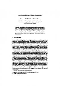
Figure 1: Architecture refinement in system design Figure 1 shows how a specification model is refined to an architecture level model with communicating components in a parallel composition. Each task in the specification is mapped to a unique component in the architecture. The model generation algorithm, presented and proved in this paper, takes the functional specification and the mapping decision as its input. The output model carries behavior inside each of the components, that can be either compiled to assembly code (for a SW component) or synthesized to RTL (for a HW component). The rest of the paper is organized as follows. Section 2 will cover system level modeling constructs. Section 3 will present the architecture refinement algorithm. Section 4 will present notions of equivalence and functionality preserving model transformations followed by the proof of correctness for architecture refinement. Experimental results are shown in section 5. We will finally wind up with conclusions and future work.
v
b1
ms
a1
(a)
b1 q1 b1
b q2 qn b2 bn
a2
(b) b1 q1
b
v1
b2
c
q1
s2 v 2 b3
b2 q2 q' 2
(c) b1 q1
2.2 Notations
s1
b2
c
v3
q2
b4
q
3
q' 3
b2 q2
t2 q'1
b
t1
(d)
(e)
Figure 2: Modeling constructs and an example functional specification model ms
2.
SYSTEM LEVEL MODELING
Formally, a model is a set of objects and composition rules defined on the objects [2]. A system level model would have objects like behaviors for computation and channels for communication. The behaviors can be composed as per their ordering . The composition creates hierarchical behaviors that can be further composed. Interfaces between behaviors and channels or amongst behaviors themselves can be visualized as relations.
2.1 Modeling constructs The various modeling constructs are shown in figures 2(a) through 2(d). Figure 2(a) shows data transaction between two parallel behaviors being realized through a channel. The channel implements two way blocking semantics, where both the sender and receiver wait until the transaction is completed. Data transfer between sequential behaviors is realized through ports. Figure 2(b) shows an ordered relation between behaviors. During execution, behavior bi , 1 ≤ i ≤ n may start executing after b has completed and condition qi is TRUE. Similarly, in figure 2(c) behavior b may start executing if either b1 is complete and q1 is TRUE or b2 is complete and q2 is TRUE. In figure 2(d), the 4 construct blocks the execution of b until both b1 and b2 have completed and both q1 and q2 evaluate to TRUE. Behaviors are either leaf-level(atomic) or hierarchical. Hierarchy is created either by parallel composition, like behavior a1 in figure 2(e), or ordered composition like behavior a2 . The parallel execution semantics ensure that a1 completes execution when both b1 and b2 are complete. The ordered composition indicates that a2 starts with start behavior s2 and completes when terminate behavior t2 has completed. Child behaviors in ordered composition have arbitrary control amongst them like conditions and loops. Further, we introduce the notion of identity behaviors. An identity behavior is a leaf level behavior that does not perform any computation, and therefore its output is the same as its input. Such behaviors may be used for synchronization or retransmission of data. The start and terminate behaviors in ordered compositions are identity behaviors.
In order to express system models succinctly, we will use some simple notations. Hierarchical behaviors are expressed as functions of child behaviors. For instance, the parallel composition representing a1 in figure 2(e) is written as a1 : ρ(b1 , b2 ). The ordered composition for behavior a2 is written as a2 : o(s2 , b3 , b4 , t2 ). Control relations representing conditional execution of behaviors are written as q.b1 ; b2 , suggesting that b2 may start after b1 is complete and q is TRUE. If the execution order is unconditional, that is b2 always executes after b1 , we write it simply as b1 ; b2 . Data transfer through ports is written as v.b1 → b2 , suggesting b2 reads the data item v written by b1 . Transactions over channels are expressed with a pair of relations as {v.b1 → c, v.c → b2 }, meaning that data v is sent from b1 to b2 over channel c. For the scope of this paper, we will use b and e for non-identity and identity behaviors respectively. Symbols q, v and c with suffix will be used for control conditions, data variables and channels respectively. Using the above notation and the basic concepts of hierarchy, control and data flow, a system model m may be written as a three-tuple : m :< H(m), C(m), D(m) >, where H(m) is the expression for the hierarchical composition of behaviors in m, C(m) is the set of control relations in m and D(m) is the set of data flow relations in m. The functional model ms in figure 2(e) is thus written as follows. H(ms ) C(ms )
= o(s1 , a1 : ρ(b1 , b2), a2 : o(s2 , b3 , b4 , t2 ), t1 ) = {s1 ; a1 , a1 ; a2 , q1 .a2 ; a1 ,
D(ms )
q10 .a2 ; t1 , s2 ; b3 , q2 : b3 ; b4 , q20 .b3 ; t2 , q3 .b4 ; b4 , q30 .b4 ; t2 } = {v1 .b1 → c1 , v1 .c1 → b2 , v2 .b2 → b3 , v3 .b2 → b4 }
3. DERIVING ARCHITECTURE MODEL The goal is to generate a model that represents the mapping of system functionality to architecture components. The specification model is an arbitrary hierarchy of behaviors representing the system functionality. Model refinement would distribute the behaviors onto components that run concurrently in the system. It must be noted that refinement does not in any way influence the mapping decision. The designer is free to choose any mapping of behaviors to components and refinement would produce a model that represents it. However, each leaf behavior in the specification model must be mapped to only one component. In order to derive an architecture model ma from a specification model ms , we use the designer decision of behavior mapping . The mapping can be written as a grouping of non-identity leaf behaviors in ms . Let {b1 , b2 , ...bn } be the non-identity leaf behaviors of ms . We can write H(ms ) = fs (b1 , b2 , ...bn ), where fs is some function using the parallel and ordered composition rules. Let the system architecture consist of k components. Let compi be the set of leaf behaviors mapped to ith component. The construction of architectural model ma for a given mapping is shown in the following algorithm. An intuitive explanation of the refinement process is as follows. We start by copying the behavior hierarchy of ms onto behaviors pe1 through pek , that represent the processing elements executing in parallel. Rename the sub-behaviors under each PE to reflect the mapping. For instance, b1 copied under pe2 is renamed as b12 . In order to realize the behavior
Algorithm 1 Generate Architecture Model 1: H(ma ) = ρ(pe1 , pe2 , ..., pek ) 2: C(ma ) = {} 3: D(ma ) = D(ms ) 4: for i = 1 TO k do 5: for j = 1 TO n do 6: if bj ∈ compi then 7: bji = o(sji , bj , zji , tji ) 8: zji = ρ(ej1 , ej2 , ..., eji−1 , eji+1 , ..., ejk ) 9: C(ma ) = C(ma ) ∪ {sji ; bj , bj ; zji , zji ; tji } 10: else 11: bji = ρ(e0ji ) 12: D(ma ) = D(ma ) ∪ {0.eji → cji , 0.cji → e0ji } 13: end if 14: end for 15: for all q.x ; y ∈ C(ms ) do 16: C(ma ) = C(ma ) ∪ {q.xi ; yi } 17: end for 18: pei = f (b1i , b2i , ..., bni ) 19: end for 20: for all v.bi → bj ∈ D(ms ), bi ∈ compl , bj ∈ compr do 21: if l 6= r then 22: D(ma ) = D(ma ) − {v.bi → bj } 23: D(ma ) = D(ma ) ∪ {v.bi → eir , v.eir → cv , v.cv → e0ir , v.e0ir → bj } 24: end if 25: end for
ma pe1
v
s11
1
a11
s 12 a12
b11
s11
b22
b12
b21
b1
v2 cv2
e'
21
e12
v2
e'12
e21
c11 a
21
s 21
22
q
b32 1 q
v2
c31
t 31 q 2 b41
q' 2 e'
41
t
c42
21
11
v3
b42 q b 2 4 q 3
t 42 q' 3 t
q' 1 t
2 s42
e41 v2
q 3
q' 3 q' 3
q 1
e'
32
b3 e32
s 22
v2
b31 s 31
q' 2
s22 b2
t 22
t 11
a
pe 2
c
22 q' 1
t 12
Figure 4: Architecture model ma b j mapped to pe i
4. PROOF OF CORRECTNESS
s ji b j1 e'j1 vj1 q' c j1 3
1
b ji
bj
b jr 1
v jr v j1
ej1
e jr
ejk
e'jk q' 3
q' 3
c jk 1
pe1
cjr
b jk
e' jr
t
ji
v jr
vjk
v jk
per
pe k
pe i
Figure 3: Architecture refinement applied to a single behavior
mapping and to preserve the original control flow, we modify leaf behaviors under each PE as follows. If bj is mapped to compi , then in the hierarchy under pei , replace bj by a sequential composition bji = o(sji , bj , zji , tji ), where zji is a parallel composition of k − 1 identity behaviors as shown in figure 3. Each of these identity behaviors is responsible for sending a message to other components that bj has completed execution. For remaining components, replace bj in the respective hierarchy by an identity behavior that receives the message for bj ’s completion. Finally, all data transfers across components are routed through the identity behaviors used for synchronization. Intra-component data transfers are preserved as is. The architecture model for the example in figure 2(e), as derived by the refinement algorithm is shown in figure 4. In this particular model, the designer choose two components PE1 and PE2 for the system architecture. Behaviors b1 and b3 are mapped to PE1, while b2 and b4 are mapped to PE2.
In order to prove correctness of the above model refinement algorithm, we must establish a notion of functional equivalence. This requires a definition of model execution semantics. Further, we present transformations that generate functionally equivalent models. The transformations are then used to present a proof of correctness.
4.1 Model execution semantics The execution of a model is best understood by unfolding it as shown in figure 5(a). We construct a (possibly infinite) directed acyclic graph (DAG) representing all possible execution scenarios. Note that in this DAG, we have flattened the model. As a result of this flattening, the parallel composition (behavior a) is now modified to an equivalent partial order (s3 ; b1 , s3 ; b2 ). A synchronization node is added to ensure that the execution of t3 does not proceed until both b1 and b2 are complete. The label on the edges connecting behavior nodes are boolean variables or boolean constants, representing conditions for a behavior to execute. By default, the unlabeled edges represent a TRUE path. The index of the conditions represents the particular instance. A behavior node will execute if all its predecessors in the DAG have executed and all the incoming condition arc labels evaluate to TRUE. Input and output data associated with behaviors is also shown with incoming and outgoing variable arcs respectively.
4.1.1 Action graph A behavior execution is further divided into three ordered sets of actions. First, the behavior reads all the input data (represented by b.rd(v)). Then the behavior executes its
start
start
s1.ex() s3.ex() s1
b1.rd(v2)
s3 v1 c
b1
b2 v2
b2.ex()
t3.ex()
s2
s2.ex()
b2.wr(v5)
b1.wr(v3)
b3.rd(v2)
v2
b3
b3ex()
q2'(1)
q2(1)
q2(1)
b4
t2 q3'(1)
q1(1)
t2
s3
q1'(1)
q1(2)
q1'(2)
s3
t1
t1
q3(1)
q1(1)
s3.ex()
q3'(1)
b4.rd(v3)
t2.ex()
b3ex()
q1'(1)
t1.ex()
b4.rd(v3)
q1'(2)
q1(2)
t1.ex()
s3.ex()
b2 v2
t2.ex()
b4.ex()
b4.ex()
v1 c
b3.rd(v2)
q2'(1)
b4.rd(v3)
v3
b1
b2.ex() b2.rd(v1)
b2.wr(v5)
t3
v3 q3(1)
b1.ex()
b2.rd(v1)
v3
b2.rd(v4)
b1.wr(v1)
b1.ex() b1.wr(v3)
b4
b1.rd(v2)
b2.rd(v4)
b1.wr(v1)
b4.ex()
v3
b1.rd(v2) t3
b2.rd(v4)
b1.wr(v1)
b1.rd(v2)
b1.ex()
b2.wr(v5)
b1.wr(v3)
b1.wr(v1) b1.ex()
t3.ex()
(a)
b2.rd(v4)
b2.ex() b2.rd(v1)
(b)
Figure 5: (a)Unfolded execution graph and (b) Action graph for specification model ms main body (represented by b.ex()). Any data transactions on the connected channels also take place interleaved with b.ex(). Finally, the behavior writes to all its output variables (represented by b.wr(v)). Note that the channel write and read actions are ordered as write followed by read, in compliance with the blocking channel semantics. Hence, we derive an action graph from the model execution graph as shown in figure 5(b) for our example.
4.1.2 Partial order trace A model execution instance is simply a valuation of the conditional variables in the action graph. Given such a valuation, we can derive a partial order trace graph as shown in figure 6. In this particular execution instance, we have assumed a valuation to be {q2 (1) = T, q20 (1) = F, q30 (1) = T, q3 (1) = F, q1 (2) = T, q10 (2) = F, ...}. Note that this trace contains only observable actions. Therefore all actions associated with identity behaviors are removed.
4.2 Equivalence of Models We define functional equivalence of two models based on the above execution semantics. Two models are equivalent if they have the same 1. leaf level non-identity behaviors, 2. conditional variables, and 3. partial order trace for same valuation of conditions. The equivalence of two models, say m1 and m2 , by the above definition is written as m1 ↔ m2 . Note that we define functional equivalence which is relevant for asynchronous system level models. Thus there is only a qualitative notion of time instead of a quantitative one. As models are refined towards greater detail, timing becomes more accurate and thus can-
b2.ex() b2.rd(v1)
b1.wr(v3)
b2.wr(v5)
Figure 6: Partial order trace for an execution instance
not be used quantitatively as a factor for equivalence.
4.3 Functionality preserving transformations Considering the definition of functional equivalence, it can be seen that comparing two independent models for equivalence is intractable due to the potentially infinite size of the partial order traces. However, we can define some simple transformations on a model that produce functionally equivalent models. New models derived by applying a sequence of these transformations would thus be equivalent to the input model by induction. Figure 7 lists a set of model transformations that preserve functionality. We now provide some intuition into the soundness of these transformations. Transformation T1 is sound by the semantics of parallel composition. A parallel composition can be turned into a partial ordered one by allowing all child behaviors to start together. Synchronization is then added to ensure that execution of the hierarchical behavior does not complete until all child behaviors are complete. T2 replaces a control relation to a hierarchical ordered behavior with a control relation to its start behavior. Similarly, T3 replaces a control relation from a hierarchical ordered behavior with a control relation from its terminate behavior. By definition, the start and terminate behaviors are always the first and last, respectively, to be executed in an ordered composition. Thus both T2 and T3 are sound. Transformation T4 flattens the hierarchy by removing a second level ordered composition that does not have any control relations. Since a hierarchical behavior itself is not observable in a partial order trace, it can be removed if it does not influence execution of other behaviors.
x a
s
x b1
T1
b2
a b1
b2
t y
y
T2
a
b
b
T3
s
a
b
t
a s
a s
b
t
t a
s a1
b1
s1
T4
T5
b1
T6
b1
b2
a
s
b1
s1
t1
t1
t
t
q 1
s
t
q e
2
b2
b1
q1 b2
b1
q1
q2
q1
q2
b2
b2
b2
q2
T7
e1
e2
e1
e2
e1
0
c
0
e2
v
T8 T9
e1
b1
v
e
v
b2
b1
v
c
v
v
e2
b2
Figure 7: Model transformations The LHS of T5 implies that if both conditions q1 and q2 are TRUE, then the behaviors b1 , e, and b2 are executed in that order. Since actions of identity behaviors are not included in the partial order trace, it is same as the trace for RHS, where y is executed after x if q1 ∧ q2 is TRUE. The LHS of T6 has two control relations, both leading from b1 to b2 . If either of the condition variables q1 or q2 evaluate to true, then b2 will be executed after b1 completes. This is equivalent to a single control relation (q1 ∨ q2 ).x ; y in the RHS. According to blocking channel semantics, the RHS term in T7 would ensure that e2 does not complete before e1 starts. Since the actions of identity behaviors are not observed in the partial order trace, e2 starting after e1 completes is equivalent to e2 being blocked until e1 starts. The LHS in T8 implies that action e1 .wr(v) is followed by e2 .rd(v) due to the ordering of behaviors. For the RHS, the same order of data transactions is maintained due to channel semantics. Since the actions of identity behaviors are not included in the partial order trace, the data transfer through the port is equivalent to the same data transfer through a channel transaction in this case. The soundness of T9 follows from the same logic as above. Both the LHS and the RHS represent a partial order trace with action b1 .wr(v) followed by b2 .rd(v).
4.4 Correctness of architecture refinement The proof for algorithm 1 is performed using the sound model transformations discussed in section 4.3. The refined model can be generated either through algorithm 1 or through a series of transformations. Typically, the deriva-
tion through transformations is longer, and thus less efficient, than the algorithmic step. Therefore, in the implementation of the refinement tool, we use the algorithm, more so because the intermediate models from individual transformations are not of interest. However, the transformations are essential for deriving the proof. To prove equivalence, we reduce both models to a flat canonical form. The canonical representation of the architecture model is then simplified to optimize away redundant identity behaviors and channels. After optimization, the canonical form representation of the architecture model is reduced that of the specification model.We present here an intuitive version of the proof for lack of space. The canonical form of a given model m is derived by converting all parallel compositions in the behavior hierarchy H(m) to ordered compositions using T1. All control relations in C(m) are then reduced to control relations only between leaf level behaviors by using T2 and T3. The hierarchy is then flattened by optimizing away the hierarchical sub-behaviors in H(m) using T4. We thus get an equivalent model m0 in the canonical form. We start with models ms and ma and derive their canonical forms m0s and m0a respectively. So, we have m0s ↔ ms and m0a ↔ ma . Now consider model m0a . Given leaf level behaviors bi , bj in m0s such that q.bi ; bj ∈ C(m0s ) Let bi ∈ compl , bj ∈ compr , l 6= r. According to the refinement algorithm, we have {bi ; zil , q.e0ir ; bj } ⊂ C(m0a ), 0.eir → e0ir ∈ D(m0a ) Using T7 to replace the channel by the control condition, we get {bi ; zil , eir ; e0ir , q.e0ir ; bj } ⊂ C(m0a ), D(m0a ) = D(m0a ) − {0.eir → eir } Now, flattening zil applying T5 twice gives us {bi ; eir , eir ; e0ir , q.e0ir ; bj } ⊂ C(m0a ), = {bi ; eir , q.eir ; bj } = q.bi ; bj Now for the case when both bi and bj are mapped to the same component. Let bi , bj ∈ compl . According to the refinement algorithm, we have {bil ; bjl ⊂ C(m0a ) Flattening by T4 gives us {bi ; zil , zil ; til .q.til ; sjl .sjl ; bj ⊂ C(m0a ). Finally, applying T5 and T6 gives us {bi ; til , q.til ; sjl .sjl ; bj ⊂ C(m0a ). = {q.bi ; sjl , sjl ; bj } = q.bi ; bj Using the above rules, we can reduce all conditional relations and synchronization channels in m0a to those in m0s . We now try to reduce the data flow relations across components. Given leaf level behaviors bi , bj in m0s such that v.bi → bj ∈ D(m0s ) Let bi ∈ compl , bj ∈ compr , l 6= r. In our refinement algorithm, data transfer across components was converted to data transactions over channels. Since bi and bj were mapped to different components, we have {v.bi → eir , v.eir → cv , v.cv → e0ir , v.e0ir → bj } ⊂ D(m0a ) Using T8, the transaction over channel can be reduced to simple port transfer with control condition, giving us {v.bi → eir , v.eir → cv , v.cv → e0ir , v.e0ir → bj } = {v.bi → eir , v.eir → e0ir , v.e0ir → bj } since eir ; e0ir ∈ C(m0a ) Finally, applying T9 twice, we have {v.bi → eir , v.eir → e0ir , v.e0ir → bj }
Design Jpeg
Vocoder
Table 1: Experimental results for different system architectures Model Lines of Modified Refinement Refinement Simulation Configuration Code LOC time (auto) time (manual) time spec. 1932 0.322s arch.(2 PEs) 2841 1112 0.164s 22.24 days 0.445s arch.(3 PEs) 4155 2306 0.259s 46.12 days 0.520s arch.(4 PEs) 4342 2884 0.285s 57.68 days 0.640s spec. 9787 1.651s arch.(2 PEs) 12650 4618 0.746s 92.36 days 2.277s arch.(3 PEs) 14874 7009 2.156s 140.12 days 2.351s arch.(4 PEs) 18648 12665 10.679s 253.3 days 2.963s
= {v.bi → e0ir , v.e0ir → bj } = {v.bi → bj } Since data transactions between behaviors mapped to the same component are preserved in the architecture model, we can reduce all data flow relations in m0a to those in m0s . We thus have m0a ↔ m0s . Using the equivalence result of the canonical form , we get ma ↔ ms .
5.
EXPERIMENTAL RESULTS
In order to evaluate our claims about savings in model rewriting and validation effort, a model refinement tool was written in C++ based on the algorithm in section 3. Models were written in the SpecC language [6] and the tool was used to automatically create models for different architecture configurations. Tests were done with Jpeg encoder specification and a voice codec application based on the ETSI GSM Vocoder standard. Table 1 shows results for the tested configurations. The savings in model rewriting can be seen by comparing the effort in manual refinement versus automatic refinement. Using an optimistic metric of 50 correctly modified lines of code per person-day, manual refinement may take days or even months. In contrast, automatic refinement produces resulting model in seconds. The models were simulated on a 2 GHz Linux machine using bitmap pictures for jpeg encoding and 3.7 second speech samples for the vocoder. Average simulation times per picture/voice sample are given in Table 1. Simulation overhead is calculated as the extra time for simulating architecture models over functional specifications. It can be seen that as the architecture becomes more complex, the simulation overhead increases. Moreover, the architecture model becomes difficult to debug due to several concurrent threads resulting from independently running components.
6.
CONCLUSIONS AND FUTURE WORK
In this paper, we presented a method for generating an architecture level model from a functional specification model and proved its correctness. We established a notion of functional equivalence in the form of partial order traces and functionality preserving transformations were defined on system level models. Finally, the refinement algorithm was proven to be correct using these transformations. The generated architecture model can be used in several ways. The resulting data transaction channels at the top-level can provide estimates of communication traffic. This information can be used in building an optimal communication architecture. Also, the generated code for each of the components can be used as reference code either for software generation
Simulation Overhead 38.2% 61.5% 98.8% 37.9% 42.4% 79.5%
on processors or HDL code generation on HW components. In the future, we would like to enhance our scheme by extending the modeling constructs and the set of sound transformations. We can, thus, prove correctness of more design steps like system scheduling and communication synthesis.
7. REFERENCES [1] SystemC, OSCI[online]. Available: http://www.systemc.org/. [2] S. Abdi and D. Gajski. System Debugging and Verification: A New Challenge. Technical Report ICS-TR-03-31, University of California, Irvine, October 2003. [3] R. Camposano. Behavior-preserving transformations for high-level synthesis. In Proceedings of the Mathematical Sciences Institute workshop on Hardware specification, verification and synthesis: mathematical aspects, pages 106–128. Springer-Verlag New York, Inc., 1990. [4] X. Chen, H. Hsieh, F. Balarin, and Y. Watanabe. Case studies of model checking for embedded system designs. In Third International Conference on Application of Concurrency to System Design, pages 20–28, June 2003. [5] W. Fokkink. Introduction to Process Algebra. Springer, January 2000. [6] D. Gajski, J. Zhu, R. Domer, A. Gerstlauer, and S. Zhao. SpecC: Specification Language and Methodology. Kluwer Academic Publishers, January 2000. [7] C. Hoare. Communicating Sequential Processes. Prentice Hall, 1985. [8] Middlehoek. A methodology for the design of guaranteed correct and efficient digital systems. In IEEE International High Level Design Validation and Test Workshop, November 1996. [9] R. Milner. A Calculus of Communicating Systems. Springer, 1980. [10] S. Rajan. Correctness of transformations in high level synthesis. In International Conference on Computer Hardware Description Languages and their Applications, pages 597–603, June 1995. [11] S. Wang and S. Malik. Synthesizing operating system based device drivers in embedded systems. In Proceedings of the International Symposium on System Synthesis, pages 37–44, September 2003.