Automatic Landmark Detection in Cephalometry Using a Modified Active Shape Model with Sub Image Matching Rahele Kafieh, Alireza mehri
Saeed Sadri
Department of biomedical engineering Isfahahan University of medicine Isfahan, Iran. e-mail:
[email protected],
[email protected]
Department of electrical engineering Isfahahan University of technology Isfahan, Iran. e-mail:
[email protected]
Abstract— This paper introduces a modification on using Active Shape Models (ASM) for automatic landmark detection in cephalometry and combines many new ideas to improve its performance. In first step, some feature points are extracted to model the size, rotation, and translation of skull. A Learning Vector Quantization (LVQ) neural network is used to classify images according to their geometrical specifications. Using LVQ for every new image, the possible coordinates of landmarks are estimated, knowing the class of new image. Then a modified ASM with a multi resolution approach is applied and a principal component analysis (PCA) is incorporated to analyze each template and the mean shape is calculated. The local search to find the best match to the intensity profile is then used and every point is moved to get the best location. Finally a sub image matching procedure, based on cross correlation, is applied to pinpoint the exact location of each landmark after the template has converged. On average 24 percent of the 16 landmarks are within 1 mm of correct coordinates, 61 percent within 2 mm, and 93 percent within 5 mm, which shows a distinct improvement on other proposed methods.
I.
INTRODUCTION
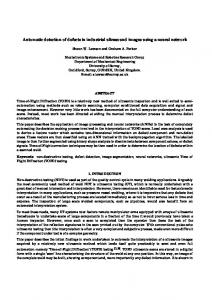
Cephalometry is a scientific measurement of dimensions of head to predict craniofacial growth, plan treatment and compare different cases. Cephalometry was first introduced by hofrath and Broadbent in 1931, using special holders known as cephalstats to permit assessment of treatment response and of growth. This analysis is based on a set of agreed upon feature points (craniofacial landmarks). The conventional method of locating landmarks depends on manual tracing of the radiographic images to locate the landmarks. There are ninety landmarks on orthodontics, thirty of which are commonly used by orthodontists [1] (Fig.1, Table.1).
Figure 1. Location of the landmarks
There have been previous attempts to automate cephalometric analysis with the aim of reducing the time required to obtain an analysis, improving the accuracy of landmark identification and reducing the errors due to clinician subjectivity. We can categorize these methods in 4 classes. The first class, being called hand crafted algorithms, usually locates landmarks based on edge detection techniques. Levy-Mandel in 1986 [2] tracked the important edges of image. They used median filter and histogram equalization to enhance the contrast of the image and to remove the noise. Based on their works, Parthasarthy in 1989 [3] presented a similar scheme and reduced the processing time by including a resolution pyramid. Yan(1986) [4], Tong(1990) [5], Ren(1998) [6] and Davis and Taylor(1991) [7] presented similar edge tracking methods. Davis and Taylor reported one of the best results of hand crafted algorithms. They defined 19 important landmarks. Their algorithm could locate seventy four percent of landmarks within 2 mm distance of correct coordinates.
All of those edge tracking methods are dependant on the quality of the x-ray and give good results for landmarks on or near to edges in the image. The second class of researchers used mathematical or statistical models to reduce the search area. Cardillo and SidAhmed (1994) [8], used sub image matching based on grayscale mathematical morphology. Seventy six percent of their 20 landmarks were located to within 2 mm. Rudolph (1998) [9] used special spectroscopy to establish the statistical gray model. They reported that 100 percent of landmarks were located to within 4 mm. Grau (2001) [10] improved the work of Cardillo and Sid-Ahmed [8] by using a line detection module to search for the most significant lines, then utilized mathematical morphology approach similar to that used by Cardillo and Sid-Ahmed [8]. Hutton (2000) [11] used Active Shape Model and reported that 35 percent of 16 landmarks were located to within 2 mm. TABLE I. Abbreviation
1 2
LIST OF THE LANDMARKS. Definition
N
Nasion, the most anterior point of the nasofrontal in the median plane
S
Sella, The midpoint of the hypophysial fossa
3
A
4
UIT
5
UIR
6
LIT
7
LIR
8
B
9
Pog
10
Gn
11
Go
12
Me
13
Po
14
Or
15
ANS
16
PNS
Point A, subspindale, the deepest midline point in the curved bony outline from the base to the alveolar process of the maxilla Tip of the crown of the most anterior maxillary central incisor Root apex of the most anterior maxillary central incisor Alveolar rim of the mandible; the lightest, most anterior point on the alveolar process, in the median plane, between the mandibular central incisors Root apex the most anterior mandibular central incisor Point B, superamentale, most anterior part of the mandibular base. It is the most posterior point in the outer contour of the mandibular alveolar process, in the median plane Pognion, most anterior point of the bony chin, in the median plane Gnathion, the most anterior and inferior point of the bony chin Gonion, a constructed point, the intersection of the lines tangent to the posterior margin of the ascending ramus and the manibular base Menton, the most caudal point in the outline of the symphysis; it is regarded as the lowest point of the mandible and corresponds to the anthropological gnathion Porion, most superior point on the head of the condyle Orbitale, lowermost point of the orbit in the radiograph Anterior nasal spine, the tip of the bony anterior nasal spine, in the median plane Posterior nasal spine, the intersection of a continuation of the anterior wall of the pterygopalatine fosa and the floor of the nose
The third class of researchers used Neural Networks, genetic algorithms and fuzzy systems to locate landmarks. Chen [12] (1999) used a combination of Neural Networks and genetic algorithms, without reporting the accuracy of landmark placement. Uchino (1995) [13] used a fuzzy machine to learn the relation between the gray levels of image and location of landmarks, but there are many problems with this method. For example they need the same size and rotation and shift for all images, and also a long training time is required. Average error of 2.3 mm was reported for this method. Innes (2002) [14] used pulse coupled Neural Networks (PCNN) to find regions containing landmarks. They tested PCNN on 3 landmarks and reported the success rate of 36.7 percent for sella, 88.1 percent for chin and 93.6 percent for nose. EI-Feghi. (2004) [15] used a combination of Neural Networks and fuzzy systems. They tested this method for 25 landmarks and reported that 90 percent of landmarks were located to within 2 mm. Chakrabartty. (2003) [16] used support vector machine (SVM) to detect 16 landmarks. They reported a success of 95 percent. Recently the 4th class of researchers are using a combination of those three classes. Yue.(2006) [17] divided every training shape to 10 regions, and for every region, Principal component Analysis (PCA) is employed to characterize its shape and gray profile statistics. For an input image, some reference landmarks are recognized and the input shape is divided using the landmarks, and then landmarks are located by an active shape model. They reported that 71 percent of landmarks were located to within 2 mm and 88 percent to within 4mm. In this paper, our method can be classified as the 4th class of researches.
II.
MATERIAL AND METHODS
A.
Material It is important to have a randomly selected data set without any judgment of their quality, sex, age and... . In this research 63 pre-treatment cephalograms were used, which were collected by hutton [11] and were accessible for comparison by other researchers. The cephalograms were scanned using a Microteck scan Maker 4 flatbed scanner at 100dpi (1pixel = 0.25mm). A drop-one-out algorithm is used for evaluate results of this method. In this algorithm, each time one of the 63 images is excluded for the test and the algorithm works with the remaining 62 images. So the algorithm can be incorporated 63 times and the mean error is reported as total error. B. Method Overview Six steps are incorporated in the proposed method. In first step, some features were extracted to model the size, rotation and translation of skull and related landmarks. A non linear diffusion filter [18] was used to remove all unwanted
noisy structures, and then a susan edge detection [19] was applied, followed by a morphological opening on the image. Then three important points were localized (Fig.2).
After detecting the three important points, some measurement features are calculated using their coordinates. These features are described in Fig.4. The second step of algorithm is applying a data clustering on measurement features, to classify cephalograms according to their geometrical specifications. A k-means clustering was used for this dataset and the algorithm converged to 5 distinct clusters. Inputs of this clustering system are features of Fig.4, which were normalized with GoN as the unit length.
Figure 4. Calculating some measurement features.
Figure 2. a) Real Cephalogram, b) After non linear diffusion, c) Susan edge detection on real cephalogram, d) Susan edge detection on image b.
Point Me, was simply located by scanning the image diagonally. The second point, N, was localised in two steps. First the image was scanned horizontally from right to left (to find the first point in frontal bone), and then the image was traced downwards to find the point with the least radius of curvature. The last point, Go, was localized by tracing the point Me towards the left ,looking for the least radius of curvature, which is the point Go [17] (Fig.3).
In the third step, we propose that results of k-means clustering be used as a target for training the LVQ Neural Networks. From now on, every test image can be evaluated with trained LVQ network to be classified in one of those 5 clusters. The fourth step of this method is estimating the possible coordinates of landmarks for every new image. In order to do this, knowing the correct cluster of each new image (in step 3), all of the training images of that cluster were aligned to the new image and for every landmark the average of coordinates on aligned training images were calculated. Alignment procedure in this step can be done having coordinates of 3 important points and with a linear conformal alignment (Fig.5).
Figure 3. Automatic detection of points Me, Go and N. Figure 5. Estimation of coordinates.
Figure 6. The complete annotated structure broken to some smaller structures.
The fifth step of algorithm is a modified Active Shape Model (ASM). The key difference between this method and a conventional ASM [11, 20] is the start shape. In a conventional ASM the start shape is the same as mean shape calculated from the training set. While in this modified ASM the start shape passes through some closer points to the correct landmarks position and increases the probability of convergence to correct position. So the mean shape changes in a way that passes through the estimated coordinates of landmarks (in step 4). In order to change the mean shape to fit the estimated landmarks, the complete annotated structure should be broken to some smaller structures, which can be considered to be independent from each other and each of them passes through (at least) 3 of estimated landmarks. Now there are 3 points in each sub image, so that affine alignment which consists of 3 equations, can be used on them (Fig.6).
In final step, a pattern matching algorithm is proposed to pinpoint the exact location of each landmark after ASM has converged. In the following, three different methods are proposed to get the best match. All of these methods were based on 2D cross correlation of a template and the image, in a window around the estimated position of landmarks. After the 5th step has converged, a small window around the last position of each landmark has the highest possibility of landmark existence and should be searched to pinpoint the exact location of landmark. The result is that there is a template which represents each landmark. Then, by moving the template over the image and calculating cross correlation between them, the point with the highest correlation value was selected as the exact place of landmark. The above mentioned method can be arranged as following: •
Rotate each template with five degrees of rotation: ±2.5, ±5, 0. (there will be five copies for each template.) Construct a weighted linear sum of the above five templates as new template space. Then find the 2D cross correlation of selected window of test image with new template space [22] (fig.8).
•
Perform a half toning on the image and template to change the gay scale picture to binary (without threshold and losing features), then construct template space and use 2D cross correlation as above.
•
Use a nonlinear diffusion, susan edge detector and a morphological opening on search window and the template, then construct template space and use 2D cross correlation as above (Fig.9).
The training set of input images which are annotated by the expert are used, firstly to calculate their mean shape with a Procrusters algorithm [17] and secondly PCA (Principal Component Analysis) was incorporated to find the main eigenvectors of the set and characterize its shape and gray profile statistics. Now to find the best match to the intensity profile, start shape is overlaid on the image and the local search is performed to move each point to get the best location (Fig.7). In this paper, a multi resolution approach [21] was used to reduce the errors and get the better fit.
Figure 8. Constructing template space in first method.
Figure 9. Constructing template space in third method.
Figure 7. a)The mean shape, overlaid on image, b)The mean shape after alignment with estimated coordinates, c)After convergence of ASM algorithm.
III.
TABLE II.
RESULTS
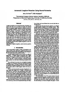
As it is illustrated in Fig.2, the results of first step which is a novel method on cephalograms shows a distinct improvement on other similar works, which is the result of strong ability of the algorithm in removing unwanted noisy structures. An LVQ neural network is proposed to be used for classification in our algorithm. The most important advantage of this method is in cases where we are in lack of enough big training set. Yue [17] proposed a method to measure the similarity between new image and all the training images (a big enough set of around 250 images), by Euclidian distance between their feature vectors (Fig.4). For an input image, the top 5% most similar images in training set were selected to be aligned and averaged to estimate the landmark locations. But where datasets are small (like the one in this paper), it is possible to have just 1 or 2 really similar images to the new image and all of 5% of images (for example 4 images), are not really similar which makes the estimated results unacceptable (Fig.10). Results of estimation in this method shows if we stop the algorithm in this step, the mean error will be about 3.4 mm. If the algorithm stops in fifth step, the mean error of landmark locating with modified ASM will be about 2.8 mm. Comparing to a conventional ASM [11], the error rate is improved about 5.5mm. (The mean error rate was 8.3 mm for conventional method.) Finally in pattern matching step we have 3 different methods. In first method, the mean error gets 2.1 mm but takes a long time to calculate the results. In second method, although the complexity of calculation decreases but the error rate becomes 2.4 mm. The best method is the third one with an error rate of 1.9mm. Although using non linear diffusion takes a long time and is a complex filtering algorithm, but this procedure is applied in first step and there is no need to be repeated.
Methods Hutton's method Yue's method Our method
COMPARISON OF RESULTS.
Within 1mm 13% Not reported 24% IV.
Recognition Rate Within Within 5mm 2mm 35% 75% 57% 61%
Around 88% 93%
DISCUSSION
This paper introduces a modification on using ASM for cephalometry and combines many new ideas to improve its performance. There are many parameters in this method, which should be studied and optimized later. Among which are two parameters of non linear diffusion, two parameters of susan edge detector, size and shape of structuring element in morphological opening and many other parameters. Also many other methods can be evaluated, like fuzzy clustering, using template matching during ASM (not after convergence), and classifying the images to different classes of gray profile of whole image to take the best and proper gray template in template matching step and finally using other model based approaches like AAM and medial profiles. V.
CONCLUSIONS
In order to evaluate the results of this method, 63 randomly selected images were used with a drop-one-out method. In each image we are looking for 16 landmarks. On average 24 percent of the 16 landmarks are within 1 mm of correct coordinates, 61 percent within 2 mm, and 93 percent within 5 mm, which shows a distinct improvement on other proposed methods as described in table.2. ACKNOWLEDGMENT R. Kafieh thanks D.D.S. Ramin Kafieh for his useful guides in dental problems, and also acknowledges the Eastman Dental Institute as the source of the cephalogram images. REFERENCES [1] [2]
[3] Figure 10. Patterned circle: new test object, Ellipse: wrong classification, Rounded rectangle: correct classification.
[4]
T Rakosi, An Atlas and Manual of Cephalometric Radiology. London, U.K.: Wolfe Medical, 1982. M Luevy-Mandel, A Venetsanopoulos and J Tsotsos, “Knowledge based landmarking of cephalograms,” Comput. Biomed , vol. 19, pp. 282–309,1986. S Parthasaraty, S Nugent, PG Gregson and DF Fay. “Automatic landmarking of cephalograms,” Comput. Biomed vol. 22, pp. 248– 269,1989. CK Yan, A Venetsanopoulos and E Filleray. “An expert system for landmarking of cephalograms,”Proceedings of the Sixth International Workshop on Expert Systems and Applications, pp. 337–356. 1986
[5]
[6]
[7] [8]
[9]
[10]
[11]
[12]
[13]
[14]
[15]
[16]
[17]
[18]
[19] [20]
[21]
[22]
W Tong, S Nugent, P Gregson, G Jesen, and D Fay. “Landmarking of cephalograms using a microcomputer system,” Comput. Biomed, vol. 23, pp.358-397, 1990. J Ren, D Liu, and J Shao. “A knowledge-based automatic cephalometric analysis method,” In Proc. 20th Annu. Int. Conf. IEEE Engineering in medicine and biology Soc. pp. 123-127 1998. D Savis and C Taylor. “A blackboard architecture for automating cephalometric analysis,” Med. Inf. vol. 16, pp. 137-149, 1991. J Cardillo, M Sid-Ahmed. “An image processing system for locating craniofacial landmarks,”IEEE Trans. Med. Imag, vol. 13, pp. 275-289, 1994. D Rudolph, P Sinclair, and J Coggins. “Automatic computerized radiographic identification of cephalometric landmarks,” Am. J. Orthod. Dentofec. Orthop, vol.113, pp. 173-179, 1998. V Grau, M Juan, C Monserrat, and C Knoll,“Automatic localization of cephalometric landmarks,” J. Biomed. Inf. vol. 34, pp.146-156, 2001. TJ Hutton, S Cunningham, and P Hamrnond. “An evaluation of active shape models for the automatic identification of cephalometric landmarks,” European Journal Orthodontics , vol.22,pp. 499–508, 2000. Y Chen, K Cheng, and J Liu. “Improving cephalogram analysis through feature subimage extraction,” IEEE Eng. Med. Biol. Mag. Vol.18, pp. 25-31, 1999. E Uchino and T Yamakawa. “High speed fuzzy learning machine with guarantee of global minimum and its application to chaotic system identification and medical image processing,” Proceeding of Seventh International Conference on tools with Artificial Intelligence. pp.242-249, 1995. A Innes, V Ciesielski, J Mamutil, and S John. “Landmark detection for cephalometric radiology images using pulse coupled neural networks,” Int. Conf. in computing in communication , pp. 391-396, 2002. I El-Feghi, S Huang, MA Sid-Ahmed and M Ahmadi. “X-ray Image Segmentation using Auto Adaptive Fuzzy Index Measure,”The 47th IEEE International Midwest Symposium on Circuits and Systems, pp. 499-502, 2000. S Chakrabartty, M Yagi, T Shibata, and G Gawenberghs. “ Robust cephalometric landmark identification using support vector machines,” in Proc. Int. Conf. Multinedia and Expo, pp. 429-432, 2003. W Yue, D Yin, CH Li and G Wang. “Locating Large-Scale Craniofacial Feature Points on X-ray Images for Automated Cephalometric Analysis,” IEEE 2005. P Mr´azek. “Nonlinear Diffusion for Image Filtering and Monotonicity Enhancement,” Available at ftp://cmp.felk.cvut.cz/pub/cmp/articles/mrazek/Mrazek-phd01.pdf SM Smith. “SUSAN Low Level Image Processing,” Available at : http://users.fmrib.ox.ac.uk/~steve/susan. T F Cootes and C J Taylor. “Active shape models,” In D. Hogg and R. Boyle, editors, 3rd British Machine Vision Conference,pp.266–275, 1992. T F Cootes and C J Taylor, and A Lanitis. “Active shape models : Evaluation of a multi-resolution method for improving image search,” In E. Hancock, editor, 5th British Machine Vison Conference, pp. 327–336, 1994 . K Tanaka, M Sano, S Ohara , and M Okudira. “A parametric template method and its application to robust matching,” Proc. of IEEE Conf. on Computer Vision and Pattern Recognition , pp. 620627, 2000.