Automatic Multi-Objective Optimization of Parameters for ... - ULBS

Automatic Multi-Objective Optimization of Parameters for Hardware and Code Optimizations Ralf Jahr, Theo Ungerer

Horia Calborean, Lucian Vintan

University of Augsburg Institute of Computer Science Universitaetsstr. 6a, 86159 Augsburg, Germany Email: {jahr, ungerer}@informatik.uni-augsburg.de

”Lucian Blaga” University of Sibiu Computer Science & Engineering Department E. Cioran Str., No. 4, Sibiu - 550025, Romania Email: {horia.calborean, lucian.vintan}@ulbsibiu.ro

Abstract—Recent computer architectures can be configured in lots of different ways. To explore this huge design space, system simulators are typically used. As performance is no longer the only decisive factor but also e.g. power usage or the resource usage of the system it became very hard for designers to select optimal configurations. In this article we use a multi-objective design space exploration tool called FADSE to explore the vast design space of the Grid Alu Processor (GAP) and its post-link optimizer called GAPtimize. For this case study we improved FADSE with techniques to make it more robust against failures and to speed up evaluations through parallel processing. For the GAP, we present an approximation of the hardware complexity as second objective besides execution time. Inlining of functions applied as a whole program optimization with GAPtimize is used as example for a code optimization. We show that FADSE is able to thoroughly explore the design space for both GAP and GAPtimize and it can find an approximation of the Pareto frontier consisting of nearoptimal individuals in moderate time. For the GAP, FADSE can find, due to the approximation of the complexity, more efficient configurations than the ones proposed yet. Index Terms—automatic design space exploration, multiobjective optimization, hardware complexity estimation, code optimization

I. I NTRODUCTION One of the future challenges when developing novel architectures is to cope with the increasing complexity of designs. While for early processor architectures the available number of transistors was a limiting bound the architectures proposed more recently have the freedom to use lots of hardware. Simple ideas to do this are increasing the cache sizes and replicating processor cores, which leads to multi- and manycore designs. Alternatively, novel processor architectures as for example TRIPS (with EDGE [1]), RAW [2], VEAL [3], WARP [4], or the Grid Alu Processor (GAP) can be used. The GAP combines elements of superscalar processor architectures with a coarse-grained reconfigurable array of functional units. Its goal is to speed up the execution of sequential instructions streams. All novel processor architectures expose lots of parameters, e.g. the number of processor cores, cache sizes, or memory bandwidth. Theses parameters form a huge design space. With multiple objectives and under specific constraints, as for example timing behavior or the availability and affordability of

hardware resources, good points consisting of a combination of parameters have to be found. It is getting very hard for the system designers to cope with this increased complexity. Tools for automatic design space exploration (ADSE) are very convenient for this job. One of them is FADSE (Framework for Automatic Design Space Exploration, [5]), which has its focus on processor architectures. FADSE has been developed to intelligently explore relevant sub-spaces of a huge design space using state-of-the-art evolutionary search algorithms. Therefore, it evaluates many different individuals. Each individual is formed by a set of parameters, where one value is selected for each parameter. The main goal of the DSE is to find the Pareto front regarding multiple objectives. The Pareto front consists of a set of individuals which do not dominate each other [6], i.e. no relation can be established between any two individuals (one is better on one objective, the other one is better on another objective). As processor architectures get more complex and diverse the optimization of programs by compilers and code optimizers in general also gets harder because the quality of the settings for these programs can be very different for apparently similar target platforms. Therefore, we propose an ADSE to solve this challenge, too. GAPtimize is a post-link optimizer to apply feedback-directed platform specific optimizations on binaries for the execution on the GAP. The main contributions of this paper are (1) an improved version of FADSE with higher robustness and a much higher degree of parallelism, (2) the introduction of a model to estimate the hardware complexity of different configurations of the GAP, (3) a description of the performance achievable with the GAP on configurations with varying complexities, and (4) that FADSE can also be used to find good parameters for software optimizations. Details on FADSE, GAP, GAPtimize, and the objectives used in the DSE are presented in Section II. The results of the DSE are explained in Section III. The presented work is put in context with related work in Section IV. Section V concludes the paper.

B. GAP The Grid Alu Processor (GAP) is a single-core processor architecture to speed up the execution of traditional singlethreaded instruction streams. 1 Homepage

of FADSE: http://code.google.com/p/fadse/

Instruction Cache

Instruction Fetch Unit Decode Unit

Configuration Unit

... Reg.

Reg.

ALU

ALU

ALU

ALU

Reg.

ALU

Reg.

...

ALU

...

ALU

LD/ST Unit

ALU

LD/ST Unit

ALU

ALU

ALU

...

ALU LD/ST Unit

ALU

Fig. 1.

ALU

ALU

Data Cache Management

A. FADSE The framework FADSE allows us to perform automatic DSEs using the state of the art evolutionary multi-objective algorithms implemented in jMetal [7] (NSGA-II [8], SPEA2 [9], SMPSO [10] and many others). The main characteristics of FADSE were already presented [5]; in the scope of this work it has been improved fundamentally to reduce the time needed for a DSE process and to increase its robustness. The algorithms used for the DSE have been modified to be run in a distributed manner. Creating new individuals for a new generation is decoupled from evaluating individuals, which allows running the simulations necessary for the evaluation of individuals in parallel (down to the core level). FADSE works on personal computers with commodity networks as well as on supercomputers (it was e.g. tested on an IBM HPC with 120 Intel Xeon cores running RedHat Linux). After running a DSE it is important to understand the quality of the generated results. For this task, FADSE now offers metrics that do not require the true Pareto front. It supports the calculation of the hypervolume, which is the volume enclosed between the Pareto front approximation and the axes in a maximization problem, coverage, which is the fraction of individuals from one population dominated by the individuals from another population, and the so-called seven point average distance [6]. These metrics can be used to (a) compare different DSEs and (b) to measure the progress of a certain DSE algorithm. FADSE also integrates various improvements to increase robustness which take into consideration situations when the a simulator or a computer crashes or a connection is interrupted, allowing FADSE to continue working without affecting the results. The framework was designed so that it can run almost any existing simulator by writing a specific connector. It is configured using an XML file, in which the user can configure the simulator parameters, the simulated architecture and a set of constraints (rules). These constraints are used to reduce the search space and to help the algorithm to find a quasi-optimal solution faster. For a further speed-up of explorations the improved version of FADSE can use a database to store the results of the evaluations of individuals. This allows it to reuse already calculated results which reduces the time required to find a good solution considerably. FADSE is available as open source.1

Processor Frontend

Branch Control Unit

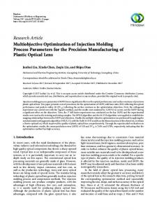
II. R ESEARCH M ETHODOLOGY AND T OOLS In the following section, we introduce the components of our case study and provide the basis for the design space exploration (DSE) by presenting parameters and objectives.

ALU

Architecture of the Grid Alu Processor

The GAP comprises a superscalar-like in-order front-end consisting of fetch- and decode-unit which is used together with a novel configuration unit. This unit is able to concurrently map independent instructions as well as data or control flow dependent instructions dynamically onto an array of functional units (FUs), a branch control unit and several load/store units to handle memory accesses (see Figure 1). The array of FUs is organized in columns and rows. Each column is dynamically and per configuration assigned to one architectural register. Every instruction is assigned to the column whose register matches the instruction’s output register. The rows of the array are used to model dependencies between instructions. A bimodal branch predictor is used to effectively map control dependencies onto the array. In order to save configurations for repeated execution all elements of the array are equipped with some memory cells which form configuration layers working similar to a trace cache. Typically, 2, 4, 8, 16, 32, or 64 configuration layers are available; the number of layers is an example for a dimension of the design space. To evaluate the architecture a cycle- and signal-accurate simulator has been developed. It uses the Portable Instruction Set Architecture (PISA) derived from a MIPS instruction set architecture; hence the simulator can execute the identical program files as the SimpleScalar simulation tool set [11]. Detailed information about the processor is given by Uhrig et al. [12] and Shehan et al. [13]. Unlike traditional architectures the GAP has been designed to be scalable, so to be able to make good use of small and large processor dies. This is mainly achieved by the different sizes of the array of FUs (from 16 to 992 FUs) as well as size and organization of the caches. The configurability of the architecture together with the ability to execute legacy code without any modification on any configuration of the GAP makes it very interesting as

candidate for a case-study with FADSE. A command-line interface has been build for the GAP simulator to invoke it with FADSE. To be able to detect unexpected behavior of the simulator and hence to ensure robustness FADSE observes an often-updated log file and compares values from this file with reference data. With the DSE, we want to find for the GAP the relation between used hardware resources and the achievable performance. Therefore, FADSE can select values for the parameters in Table I. TABLE I PARAMETER SPACE FOR GAP

Cr Cc Cl Cc1 Cc2 Cc3

Description Array: rows Array: columns Array: layers Cache: line size Cache: sets Cache: lines per set

Domain {4, 5, 6, 7, ..., 32} {4, 5, 6, 7, ..., 31} {1, 2, 4, 8, ..., 64} {4, 8, 16} {32, 64, 128, 256, ..., 8192} {1, 2, 4, 8, ..., 128}

C. GAPtimize One of the most important features of GAP is that the complete mapping of instructions, which could be understood as placement and routing, is done in hardware, hence without the need of using any special software to recompile or prepare a program for the execution on the GAP. This enables the execution of legacy code, for which source code is not available. For the evaluation of platform-specific code optimizations in this situation a post-link optimizer has been developed. Our post-link optimizer is called GAPtimize. It works on statically linked executable files compiled with GCC for PISA. GAPtimize is able to use information about the configuration of the target platform as well as performance data collected from a previous run of the program as feedback. Because of this, it can perform feedback-directed and adaptive code-optimizations. Currently, as optimizations for the GAP predicated execution, a special scheduling technique, inlining of functions, a software-assisted replacement strategy for the configuration layers [14], and static speculation [15] have been implemented. We put the focus here on the inlining of functions (also called inline expansion). In short, inlining replaces function calls with copies of the body of the called function. With this technique, the number of instruction cache misses shall be reduced because the accesses to the program data are more sequential which leads to less cache conflicts and a higher impact of prefetching. A kind of prefetching is implemented in the GAP because on an instruction cache miss the complete cache line consisting of multiple instructions is loaded into the cache. By reducing the number of function returns the number of indirect jumps is reduced, too. For the GAP, indirect jumps are very likely to lead to reconfigurations of the array which causes an additional penalty. Nevertheless, the more functions are inlined the larger

gets the memory footprint of the program and the more cache conflicts can occur simply because more areas of the memory are mapped to the same cache line. Inlining is performed by lots of compilers, for example GCC. The outstanding feature of the implementation of function inlining in GAPtimize over the implementation GCC (in the version used for GAP) is its application as whole program optimization. GAPtimize works on statically linked binaries, hence it can perform analyses and optimizations on the whole program. The main challenge is choosing the right function callers which shall be replaced by copies of the function body. For this, we developed a comparably simple heuristics inspired by work on inlining in combination with machine learning [16], [17], [18], [19]. Our heuristics exposes four parameters (see Table II). TABLE II PARAMETER SPACE FOR FUNCTION INLINING WITH GAP TIMIZE Parameter max_caller_count weight_of_caller length_of_function insns_per_caller

Domain {0, 1, 2, 3, ..., 100} {0, 1, 2, 3, ..., 100} {0, 1, 2, 3, ..., 10000} {0, 1, 2, 3, ..., 200}

Not more than max_caller_count callers are inlined by GAPtimize. Each of them must have been executed at least weight_of_caller times in a reference run. The function which is called must not be longer than length_of_function measured in static instructions. Beyond this, a classification number C for the caller must not be larger than insns_per_caller. C is the dynamic weight of the caller divided by the static number of instructions of the target function. This ratio is equal to the number of instructions which have to be added to the program in order to remove the execution of one pair of function call and return. FADSE can run GAPtimize with a command line interface; a file in YAML format is used to pass the parameters to GAPtimize. Unexpected behavior is detected by observing and analyzing the standard output. D. Objectives Used Objectives are used to describe the quality of configurations. The quality of a configuration for the GAP and GAPtimize is mainly described by the used hardware resources and the performance which can be achieved: 1) Performance: The time which has to be spent on the execution of a program is a valid candidate to measure the quality of a processor’s configuration. For this, we configure our cycle-accurate simulator with the configuration generated by the DSE algorithm and run the simulation. It counts the total number of clock cycles for the simulation and the number of instructions which it has executed. These values are used to calculate the number of clocks per instruction (CPI). The goal is to reduce this measure. It is comparable because the number of instructions is the same with every run of the program and with any configuration of the processor.

TABLE III C ONSTANTS AND THEIR VALUES TO APPROXIMATE HARDWARE COMPLEXITY OF THE GAP Constant hALU hLSU hl hr

Value 1.00 3.50 0.02 0.02

Description FU comprising an ALU Load-store unit (LSU) Configuration layer for a FU Top-register

Things are different with GAPtimize, which can change the number of instructions needed to execute the benchmark program to complete. Hence, we again measure the number of clock cycles for the program but divide it by the number of instructions executed without using GAPtimize. We call this measure clocks per reference instruction (CPRI). 2) Hardware Complexity: The GAP is very scalable, hence performance results have to be seen always in context with the used resources. To solve this, a model is needed to measure the hardware complexity of the GAP. It is not possible to use bullet-proof numbers as there is not yet a hardware implementation for the GAP available. We therefore introduce an approximation model. The targets of this model are (a) to be able to compare the hardware complexity of two configurations of the GAP and (b) compare the performance of two processors with different configurations but the same overall complexity. Hence, the purpose of the measure called complexity in the following is not to estimate the area used by the processor but to estimate the ratio between the complexities of two differently configured processors for comparison. The complexity H of the GAP is composed of the processor front-end Hf ront , the array consisting of the ALUs and the load-store units with complexities HALU s and HLSU s , the instruction cache with complexity HICache and some other components which exist exactly once in the GAP and are independent of parameters. These components contribute Hconstant ; the data cache is one of them because it is not configurable (at the moment). To conclude, H can be defined as: H = Hf ront + HALU s + HLSU s + HICache + Hconstant As we need the complexities only for comparability, we ignore Hf ront and Hconstant in the following because they are the same for all configurations of GAP. To be able to calculate the complexities of the functional units in the array we declare the constants in Table III. To find appropriate values for these constants we use the following three approaches: • The thermal simulation tool HotSpot [20] comprises a floor plan for the 64 bit Alpha 21264 processor [21]. This floor plan was gained from carefully taking the measures from a die photo from this processor. • Gupta et al. present in their article [22] numbers for several parts of a processor and try to find processindependent numbers to estimate their size.2 2 The

standard deviation of the values they used is quite high.

The combined simulator for power, area, timing and temperature McPat [23] is shipped with a configuration for the 64 bit Alpha 21364 processor which extends the Alpha 21264. The area approximation is based on the work by Gupta et al. (see above) and Rodrigues [24]. From these approaches we isolated the size of a 64 bit ALU, a 64 bit register and 64 kb of instruction cache. As the GAP is a 32 bit processor we divided the size of the ALU and the register by two; this method is supported by e.g. Gupta et al. [22]. The numbers are finally normalized to the size of an integer ALU (so, hALU := 1 for all sources); Table IV shows the results. •

TABLE IV R ATIO OF 32 BIT R EGISTER AND 64 BK INSTRUCTION CACHE COMPARED TO A 32 BIT INTEGER ALU (hALU := 1) Data Source McPat for Alpha 21364 HotSpot Alpha 21264 Gupta et al. Average

32 bit register 0.031 0.008 0.017 0.019

64 kb ICache 15.678 16.767 17.131 16.525

The results for a 32 bit register vary quite a lot between the different data sources. Nevertheless, the cost of a register is for all sources very small compared to the cost of a 32 bit integer ALU. Because of this, we set hr := 0.02. We choose as additional cost for a configuration layer the same cost hl := 0.02 although th rquired memory is double the size but of a much lower complexity. For a load-store unit numbers were available only from McPat and the floor plan, they vary between ca. 1.5 and 5.4 times the size of an integer ALU. We define hLSU := 3.5. The cost of a 64 kb instruction cache compared to an integer ALU is ca. 16.5 on average for the three data sources. CACTI [25] calculates a total area of 5.52mm2 for a cache with parameters similar to those of the alpha processors3 . To be able to use CACTI to dynamically approximate the complexity of the instruction cache HICache we set 16.5 equal to an instruction cache with a total area of 5.52mm2 . We calculate the approximated area of a cache for the GAP with CACTI and 1 1 then multiply it with 16.5/5.52mm2 = 2.99 mm 2 ≈ 3 mm2 to get its complexity compared to an ALU. With these constants, we can define the complexities HALU s and HLSU s . In both formulas, where Cc is the number of columns, Cr is the number of rows, and Cl is the number of configuration layers of the array of FUs, we first calculate the complexity of the units and then add the complexity caused by the configuration layers: HALU s = (Cc ∗ hr + Cr ∗ Cc ∗ hALU ) + Cr ∗ Cc ∗ Cl ∗ hl HLSU s = Cr ∗ hLSU + Cr ∗ Cl ∗ hl For a GAP with an array of 12 lines and columns, 32 configuration layers and 8 kb instruction cache, the hardware complexity H is computed as follows: H = HALU s + HLSU s + HICache 3 Cacti 5.3 web interface, 64 kb total size, 128 byte line size, 2-way associative, 1 bank, 90 nm technology

1,4

Manually selected

1,3 1,2

Found by FADSE

1,1 1

CPI

HALU s = (12 ∗ 0.02 + 12 ∗ 12 ∗ 1.00) + 12 ∗ 12 ∗ 32 ∗ 0.02 = 144.24 + 92.16 = 236.40 HLSU s = 12 ∗ 3.50 + 12 ∗ 32 ∗ 0.02 = 49.68 1 HICache = 0.856mm2 ∗ 3 mm 2 = 2.57 H = 236.4 + 49.68 + 2.57 = 288.65 In this work, our developed FADSE has two distinct objectives: to minimize the CPI (or CPRI, depending on the context) and to minimize the global hardware complexity (H).

0,9 0,8 0,7

III. E VALUATION

0,6

After describing our setup for the evaluation in Section III-A we show our results for the design space exploration (DSE) with the GAP in Section III-B. Results for the GAP together with GAPtimize are shown in Section III-C.

0,5 0,4 0

500

1000

1500

2000

2500

3000

Complexity

A. Evaluation Methodology

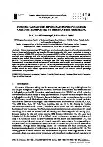
B. ADSE on GAP For every generation of size n, the NSGA-II algorithm normally knows n already evaluated individuals, the parent generation. They are used to generate with crossover and mutation n new individuals called offspring, which have to be evaluated. When this is completed, n individuals are selected from the union of the parent generation and the offspring. We initially set the population size to 100 and obtained the results in Figure 2(a) and 2(b). Slightly better results

(a) Total result space 0,700 Manually selected

0,675

Found by FADSE

0,650 0,625

CPI

A kind of DSE has been performed for the GAP by Shehan et al. [13]. In this manual exploration, 14 benchmarks from the MiBench Benchmark Suite [26] were selected. In difference to the evaluation here the instruction cache size was set to a fixed value, i.e. 8x128x1 x 8 byte = 8 kb. As result, it is suggested as rule of thumb to use the same number of lines and columns for array sizes up to 16x16. For an even larger array, it is proposed to choose 16 columns and 32 lines. In the following, these results in combination with a much larger cache are referred to as manually selected configurations. We choose NSGA-II [8] as algorithm for the DSE and run it with FADSE on the design space as described in Section II-B. With 5295 possible configurations for the array and 192 configurations for the instruction cache it comprises 1016640 individuals in total for the GAP. GAPtimize has ca. 2.1∗1010 configurations, i.e. together with GAP we get a max. design space of ca. 2.1 ∗ 1016 individuals. With the restrictions introduced later the design space to explore for GAP together with GAPtimize has a size of ca. 1.8∗1013 individuals. FADSE was run using different population sizes so the influence of this parameter could be observed on the results. The crossover probability was set to 0.9 and mutation probability to 1/(number of parameters); the distribution indexes for mutation and crossover were set to 20 as recommended [8]. We have used single point crossover and bit flip mutation operators. The selection operator is Binary Tournament as proposed by Deb et al. [8]. 10 of the 14 benchmarks used by Shehan et al. were selected as benchmarks to reduce the time needed to evaluate an individual of the design space.

0,600 0,575 0,550 0,525 0,500 0

200

400

600

800

1000

1200

Complexity (b) Zoom on most interesting area (highlighted box in Figure 2(a)) Fig. 2. Individuals of the last of 55 generations calculated with FADSE (population size 100) for GAP in comparison with results for configurations selected with the rule of thumb

were generated by FADSE than the ones obtained by the manual exploration. The main outcome is that with FADSE configurations for the GAP can be found which use much less hardware resources to achieve the same CPI as manually selected configurations. A more thorough analysis showed us that with the rule of thumb, the array normally has too many columns which cannot be used efficiently. This means that FADSE is indeed able to help the designer make better choices. The overall shape of the curve in Figure 2(a) also shows that increasing the hardware complexity above 1000 does not result in much higher performance (for the selected benchmarks). With this complexity, you can build a GAP with an array of 32 lines, 11 columns and 32 layers (i.e. 32x11x32), and 512 kb instruction cache (i.e. 16x2048x2 * 8 byte). To evaluate the influence of the population size, which is an important factor for the total duration of a DSE process, we set it to different values (12, 24, 50, and 100). For 12 and 24, we were not able to reliably find good results because the

Coverage

100%

Coverage (p100, p50)

80%

Coverage (p50, p100)

100

New individuals

80 60

Individuals added to population

40 20 0 0

10

20

30

Generation

40

50

60

Fig. 5. Comparison between the number of newly generated individuals (offspring) and the number of them that actually reach the next generation

60%

C. ADSE on GAP together with GAPtimize

40% 20% 0

200

400

600

800

1000

1200

Number of simulated individuals Fig. 3. Coverage comparison between a DSE process with a population of 100 and another one with a population of 50

The selection process of the individuals can be observed in Figure 5. The number of new individuals, i.e the individuals which have never been generated before in the exploration, decreases over time, e.g. from 100 to 35. Due to this fact, it is very effective to save results for individuals for reuse for example in a database. This can speed up the DSE very much. In a run with 100 generations a total reuse factor of 67% was observed. The number of those individuals which are better than their parents and hence survive for the next generation decreases over time, too. According to Figure 5 at the beginning of the exploration many of the offspring individuals are better than their parents, therefore they are moving into the next generation. As the algorithm progresses less and less good individuals are found. This is adequately correlated with the hypervolume, whose improvement from one generation to the next decreases (Figure 4). 0,685 0,684

Hypervolume

Number of Individuals

selection/mutation did not work effectively. To compare the progress made with generations of size 50 and 100 in respect to the number of evaluated individuals we calculated the hypervolume and coverage for each generation. The difference in hypervolume is less than 1% (only marginal). Coverage (see Figure 3) does not show a clear winner, too. A large population clearly has the benefits of a better exploration but it will also mean more simulations.

0,683 0,682 0,681 0,680 0,679 0,678 0

10

20

30

40

50

Generation Fig. 4.

Evolution of the hypervolume value over the generations

60

Because FADSE is not restricted to a single domain we also coupled it with GAPtimize, the post-link optimizer for the GAP. As case-study, we are using inline expansion of functions and a simple heuristics (see Section II-C). To increase the potential of improvement for this code modification we first compiled the benchmarks without inlining functions (i.e. -fno-inline). From a prior thorough analysis we know that improvements are mainly caused by making instructions accessible faster. This can be because they are either in the instruction cache or, as complete configuration, on a configuration layer. Because of this, a GAP with a large instruction cache or many configuration layers will profit from inline expansion only marginally. So, to see if FADSE can choose good parameters for our heuristics, we restrict the instruction cache to 8 kb and the number of configuration layers to 8. For a first evaluation we select the benchmark dijkstra, about which we know that it is sensitive to inline expansion, and run this single benchmark with GAP and an array of 12x12 functional units. Because the hardware is fixed we have CPRI as single objective. We found out that FADSE finds fitting values for the parameters; the execution time is reduced by 9.1%. As next step the number of benchmarks is increased to 10. The hardware is still fixed; it is again a single-objective optimization problem. Figure 6 shows the results. Because not all benchmarks are sensitive to inlining the reduction of the execution time is only 3.9%. To make things more complex the hardware configuration is released. FADSE has to find now in parallel efficient hardware configurations and for these configurations effective parameters for the inlining heuristics (Figure 7 for dijkstra and Figure 8 for 10 benchmarks). It can cope with this challenge very well. It can be concluded that the proposed heuristics is general enough to select with a single set of parameters and for a given hardware configuration a good set of function calls also for multiple benchmarks. In other words, FADSE was in connection with the heuristics able to perform inlining as an adaptive code optimization.

1,09

CPRI

1,08 1,07 1,06 1,05 1,04 0

5

10

15

Generation

20

Fig. 6. DSE of the inlining parameters for 10 benchmarks, executed on GAP with 12x12x8 array and 8 kb instruction cache. The dotted grey line is the CPRI without inlining.

CPI / CPRI

1,7

CPRI (HW+SW)

1,6

CPI (HW)

1,5 1,4 1,3 1,2

V. C ONCLUSION AND F UTURE W ORK 0

100

200

300

400

500

Complexity

600

700

800

Fig. 7. DSE of inlining and hardware parameters for benchmark dijkstra, executed on GAP with NxNx8 array and 8 kb instruction cache

IV. R ELATED W ORK As mentioned before there is no prior work on the approximation of the hardware complexity of the GAP. The presented design space exploration (DSE) is also the first multi-objective one for this processor. With respect to FADSE there are existing tools which try to address the problem of automatic DSE in the domain of processor architectures. One of them is Magellan [27] which focuses on multi-core architecture. From our point of view, the main drawbacks of this tool are that it is bound to a certain simulator (SMTSIM) and that it is not multi-objective in a true way. The user can set a boundary for its power/area ratio but 1,25

CPI / CPRI

cannot explore the entire Pareto front in a single run. Archexplorer.org [28] is a collaborative website where users can upload components of processors contributing to a DSE with the goal to find an optimal processor. The used algorithms cannot be controlled and the tool is strongly related to UNISIM (at the moment), hence it cannot be used for a different processor simulator easily. NASA [29] also shows similarities. It can connect to any simulator, it is extensible, but it does not provide many DSE algorithms yet. The authors present only one self-developed single-objective algorithm and suggest that multi-objective algorithms could be implemented. It lacks a technique for the distributed evaluation of individuals, too. M3Explorer [30] offers a variety of multi-objective DSE algorithms, but it lacks the distributed simulation. As conclusion, even though parallel algorithms exist and although sequential evolutionary algorithms can be parallelized easily, none of the presented tools shows this ability. This and its configurability are strong advantages of the improved version of FADSE introduced in this article to reduce the time needed for a DSE dramatically.

CPRI (HW+SW)

1,2 1,15

CPI (HW)

1,1 1,05 1 0,95 0

100

200

300

400

500

Complexity

600

700

800

Fig. 8. DSE of inlining and hardware parameters for 10 benchmarks, executed on GAP with NxNx8 array and 8 kb instruction cache

In this article, an new version of the framework for automatic design space explorations (FADSE) has been introduced. It is very configurable and can, with the improvements presented, run the simulations needed for evaluating individuals in parallel and in a distributed manner with high robustness. Increasing parallelism and buffering results leads to a strong reduction of the time needed for the exploration. With FADSE the design space of the architectural parameters of the Grid Alu Processor has been explored. To do this, we first presented an approximation of the hardware complexity of the processor. Then we approximated the Pareto frontier with respect to the two objectives performance and hardware complexity. FADSE demonstrated that GAP is scalable and bigger caches do not cancel the effects of the ALU array and the configuration layers. FADSE is also able to cope with hardware and software parameters and find good solutions even in a huge design space ( 1.8∗1013 individuals). To demonstrate this we searched with FADSE in parallel for efficient hardware configurations and effective parameters for a heuristics to performance function inlining as whole program optimization with GAPtimize. This worked very well, hence FADSE can be used for adaptive static code optimizations. As future work we propose to add an interface to FADSE so that the user can influence the DSE with preferences and expertise. Technically speaking, the user will be able to specify an ontology with relations between the parameters by describing fuzzy functions and relations between them. Beyond this, FADSE could also be extended to decide automatically if the DSE can be stopped or if improvements are still made. It would also be interesting to see how different DSE-algorithms perform and to compare their behavior automatically.

VI. ACKNOWLEDGEMENTS Lucian Vintan was supported by CNCSIS no. 485/2008 research grant offered by the Romanian National Council for Academic Research. Horia Calborean was supported by POSDRU financing contract POSDRU 7706. R EFERENCES [1] D. Burger, S. W. Keckler, K. S. McKinley, M. Dahlin, L. K. John, C. Lin, C. R. Moore, J. H. Burrill, R. G. McDonald, and W. Yode, “Scaling to the end of silicon with EDGE architectures.” IEEE Computer, vol. 37, no. 7, pp. 44–55, 2004. [2] M. B. Taylor, J. S. Kim, J. E. Miller, D. Wentzlaff, F. Ghodrat, B. Greenwald, H. Hoffmann, P. Johnson, J.-W. Lee, W. Lee, A. Ma, A. Saraf, M. Seneski, N. Shnidman, V. Strumpen, M. Frank, S. P. Amarasinghe, and A. Agarwal, “The Raw microprocessor: A computational fabric for software circuits and general-purpose programs.” IEEE Micro, vol. 22, no. 2, pp. 25–35, 2002. [3] N. Clark, A. Hormati, and S. Mahlke, “VEAL: Virtualized execution accelerator for loops,” in Proc. of the International Symposium on Computer Architecture, 2008, pp. 389–400. [4] R. Lysecky, G. Stitt, and F. Vahid, “Warp processors,” ACM Trans. Des. Autom. Electron. Syst., vol. 11, no. 3, pp. 659–681, 2006. [5] H. Calborean and L. Vintan, “An automatic design space exploration framework for multicore architecture optimizations,” in Roedunet International Conference (RoEduNet), 2010 9th, Sibiu, Romania, June 2010, pp. 202 –207. [6] C. A. C. Coello, D. A. V. Veldhuizen, and G. B. Lamont, Evolutionary Algorithms for Solving Multi-Objective Problems, 1st ed. Springer, Jun. 2002. [7] J. J. Durillo, A. J. Nebro, F. Luna, B. Dorronsoro, and E. Alba, “jMetal: a java framework for developing Multi-Objective optimization metaheuristics,” Departamento de Lenguajes y Ciencias de la Computacion, University of Malaga, E.T.S.I. Informatica, Campus de Teatinos, Tech. Rep. ITI-2006-10, Dec. 2006. [8] K. Deb, A. Pratap, S. Agarwal, and T. Meyarivan, “A fast and elitist multiobjective genetic algorithm: NSGA-II,” Evolutionary Computation, IEEE Transactions on, vol. 6, no. 2, pp. 182–197, 2002. [9] E. Zitzler, M. Laumanns, and L. Thiele, “SPEA2: Improving the strength pareto evolutionary algorithm,” Computer Engineering and Networks Laboratory (TIK), Swiss Federal Institute of Technology (ETH), Zurich, Switzerland, Tech. Rep. 103, 2001. [10] A. Nebro, J. Durillo, J. Garcıa-Nieto, C. A. Coello, F. Luna, and E. Alba, “Smpso: A new pso-based metaheuristic for multi-objective optimization,” in Proceedings of the IEEE Symposium Series on Computational Intelligence, 2009, pp. 66–73. [11] T. Austin, E. Larson, and D. Ernst, “Simplescalar: An infrastructure for computer system modeling,” IEEE Computer, vol. 35, pp. 59–67, 2002. [12] S. Uhrig, B. Shehan, R. Jahr, and T. Ungerer, “The two-dimensional superscalar GAP processor architecture,” International Journal on Advances in Systems and Measurements, vol. 3, no. 1 and 2, pp. 71 – 81, September 2010. [13] B. Shehan, R. Jahr, S. Uhrig, and T. Ungerer, “Reconfigurable Grid Alu Processor: Optimization and design space exploration,” in Proceedings of the 13th Euromicro Conference on Digital System Design (DSD) 2010, Lille, France. Los Alamitos, CA, USA: IEEE Computer Society, 2010, pp. 71–79. [14] R. Jahr, B. Shehan, S. Uhrig, and T. Ungerer, “Optimized replacement in the configuration layers of the Grid Alu Processor,” in Proceedings of the Second International Workshop on New Frontiers in High-performance and Hardware-aware Computing (HipHaC11). Strasse am Forum 2, 76131 Karlsruhe, Germany: KIT Scientific Publishing, 2011, pp. 9–16. [15] ——, “Static speculation as post-link optimization for the Grid Alu Processor,” in Proceedings of the 4th Workshop on Highly Parallel Processing on a Chip (HPPC 2010), 2010. [16] J. Cavazos and M. F. P. O’Boyle, “Automatic tuning of inlining heuristics,” in SC ’05: Proceedings of the 2005 ACM/IEEE conference on Supercomputing. Washington, DC, USA: IEEE Computer Society, 2005, pp. 14–14. [17] M. Arnold, S. Fink, V. Sarkar, and P. F. Sweeney, “A comparative study of static and profile-based heuristics for inlining,” SIGPLAN Not., vol. 35, no. 7, pp. 52–64, 2000.

[18] T. Waterman, “Adaptive compilation and inlining,” Ph.D. dissertation, Houston, TX, USA, 2006. [19] K. D. Cooper, T. J. Harvey, and T. Waterman, “An adaptive strategy for inline substitution,” in CC’08/ETAPS’08: Proceedings of the Joint European Conferences on Theory and Practice of Software 17th international conference on Compiler construction. Berlin, Heidelberg: Springer-Verlag, 2008, pp. 69–84. [20] W. Huang, M. Stan, and K. Skadron, “Parameterized physical compact thermal modeling,” Components and Packaging Technologies, IEEE Transactions on, vol. 28, no. 4, pp. 615 – 622, December 2005. [21] P. E. Gronowski, W. J. Bowhill, R. P. Preston, M. K. Gowan, Y. L. Allmon, and A. Member, “High-performance microprocessor design,” IEEE Journal of Solid-State Circuits, vol. 33, pp. 676–686, 1998. [22] S. Gupta, S. W. Keckler, and D. Burger, “Technology independent area and delay estimates for microprocessor building blocks,” University of Texas at Austin, Tech. Rep. TR2000-05, 2000. [23] S. Li, J. H. Ahn, R. D. Strong, J. B. Brockman, D. M. Tullsen, and N. P. Jouppi, “Mcpat: an integrated power, area, and timing modeling framework for multicore and manycore architectures,” in MICRO 42: Proceedings of the 42nd Annual IEEE/ACM International Symposium on Microarchitecture. New York, NY, USA: ACM, 2009, pp. 469–480. [24] A. F. Rodrigues, “Parametric sizing for processors,” Sandia National Laboratories, Tech. Rep., 2007. [25] S. Thoziyoor, J. H. Ahn, M. Monchiero, J. B. Brockman, and N. P. Jouppi, “A comprehensive memory modeling tool and its application to the design and analysis of future memory hierarchies,” in ISCA ’08: Proceedings of the 35th Annual International Symposium on Computer Architecture. Washington, DC, USA: IEEE Computer Society, 2008, pp. 51–62. [26] M. R. Guthaus, J. S. Ringenberg, D. Ernst, T. M. Austin, T. Mudge, and R. B. Brown, “Mibench: A free, commercially representative embedded benchmark suite,” in Proceedings of the Workload Characterization, 2001. WWC-4. 2001 IEEE International Workshop. Washington, DC, USA: IEEE Computer Society, 2001, pp. 3–14. [Online]. Available: http://portal.acm.org/citation.cfm?id=1128020.1128563 [27] S. Kang and R. Kumar, “Magellan: a search and machine learningbased framework for fast multi-core design space exploration and optimization,” in Proceedings of the conference on Design, automation and test in Europe. Munich, Germany: ACM, 2008, pp. 1432–1437. [28] V. Desmet, S. Girbal, A. Ramirez, O. Temam, and A. Vega, “Archexplorer for automatic design space exploration,” IEEE Micro, vol. 30, no. 5, pp. 5 –15, 2010. [29] Z. J. Jia, A. Pimentel, M. Thompson, T. Bautista, and A. Nunez, “Nasa: A generic infrastructure for system-level MP-SoC design space exploration,” in Embedded Systems for Real-Time Multimedia (ESTIMedia), 2010 8th IEEE Workshop on, October 2010, pp. 41 – 50. [30] C. Silvano, W. Fornaciari, G. Palermo, V. Zaccaria, F. Castro, M. Martinez, S. Bocchio, R. Zafalon, P. Avasare, G. Vanmeerbeeck et al., “MULTICUBE: Multi-Objective Design Space Exploration of MultiCore Architectures,” in Proceedings of the 2010 IEEE Annual Symposium on VLSI. IEEE Computer Society, 2010, pp. 488–493.