Sep 7, 2009 - We developed a framework based on the CLIF load injection framework [4] to automatically manage load injection tests and deduce a model ...
INSTITUT NATIONAL DE RECHERCHE EN INFORMATIQUE ET EN AUTOMATIQUE
Automatic performance modelling of black boxes targetting self-sizing
N° 7027
ISRN INRIA/RR--7027--FR+ENG
Juillet 2009
ISSN 0249-6399
inria-00413935, version 1 - 7 Sep 2009
Ahmed Harbaoui — Nabila Salmi — Bruno Dillenseger — Jean-Marc Vincent
inria-00413935, version 1 - 7 Sep 2009
Automatic performance modelling of black boxes targetting self-sizing Ahmed Harbaoui , Nabila Salmi , Bruno Dillenseger , Jean-Marc Vincent Thème : Modélisation et évaluation des performances des systémes distribués Équipes-Projets MESCAL
inria-00413935, version 1 - 7 Sep 2009
Rapport de recherche n° 7027 � Juillet 2009 � 19 pages
Abstract: Modern distributed systems are characterized by a growing complexity of their ar-
chitecture, functionalities and workload. This complexity, and in particular signi�cant workloads, often lead to quality of service loss, saturation and sometimes unavailability of on-line services. To avoid troubles caused by important workloads and ful�ll a given level of quality of service (such as response time), systems need to self-manage, for instance by tuning or strengthening one tier through replication. This autonomic feature requires performance modelling of systems. In this objective, we developed an automatic identi�cation process providing a queuing model for a part of distributed system considered as black box. This process is a part of a general approach targetting self-sizing for distributed systems and is based on a theoretical and experimental approach. In this report, we show how to derive automatically the performance model of one black box considered as a constituent of a distributed system, starting from load injection experiments. This model is determined progressively, using self-regulated test injections, from statistical analysis of measured metrics, namely response time. This process is illustrated through experimental results.
Key-words: Performance, modelling, queue model, load injection, black box, self-sizing
Centre de recherche INRIA Grenoble – Rhône-Alpes 655, avenue de l’Europe, 38334 Montbonnot Saint Ismier Téléphone : +33 4 76 61 52 00 — Télécopie +33 4 76 61 52 52
Vers une modélisation automatique des performance de boîtes noires pour un dimensionnement autonome
inria-00413935, version 1 - 7 Sep 2009
Résumé : De nos jours, les systèmes distribués sont caractérisés par une complexité croissante
de l'architecture, des fonctionalités et de la charge soumise. Cette complexité induit souvent une perte de la qualité de service o�erte, ou une saturation des ressources, voire même la non disponibilité des services en ligne, en particulier lorsque la charge est importante. A�n d'éviter les désagrèments causés par d'importantes charges et remplir le niveau attendu de la qualité de service, les systèmes nécessitent une auto-gestion, en optimisant par exemple un tier ou en le renforçant à travers la réplication. Cette propriété autonome requiert une modélisation des performances de ces systèmes. Visant cet objectif, nous développons un processus automatique d'identi�cation de modèle, fournissant un modèle de �le d'attente pour une boîte noire, considérée comme un constituant d'un système distribué. Ce processus fait partie d'une approche générale de dimensionnement autonome des systèmes distribués. Il est basé sur une méthodologie théorique et expérimentale. Dans ce rapport de recherche, nous montrons comment dériver automatiquement un ou plusieurs modèles de performance d'une boîte noire, partant d'un ensemble d'expérimentations d'injections de charge. Ce modèle est déterminé progressivement, en utilisant des injections auto-régulées, à partir d'analyses statistiques de mesures de performances, à savoir le temps de réponse. Ce processus est illustré à travers des résultats expérimentaux.
Mots-clés : Performance, modélisation, �le d'attente, injection de charge, boîte noire, dimensionnement autonome
Automatic performance modelling of black boxes targetting self-sizing
3
1 Introduction
inria-00413935, version 1 - 7 Sep 2009
Nowadays, distributed systems have become widespread critical infrastructures, performing critical business processes and o�ering a great variety of services. The management of such systems is being more and more complex and costly to achieve. In this context, autonomic computing [7] aims at providing systems and applications with self-management capabilities, including self-con�guration, self-optimization, self-healing and self-protection. It is based on a control loop back where a possible problem is observed, then a decision to correct the problem is taken, followed by a reaction applying the proposed decision. The decisional module should be enough precise and safe so that the proposed solution can replace e�ciently the administrator task. Consequently, a solution (con�guration) should not be applied until checking whether performances of the recon�gured system are degraded or not by this new con�guration. To ensure that, performance prediction of the target con�guration is recommended before its deployment. Performance prediction tools are based on a performance model of the system. They provide performance indexes computed through analytical or simulation methods.
Figure 1: General approach for qualifying performances of a distributed system Our global objective is to generate automatically a performance model for the system under study. The modelling process is a part of a general approach, proposed in [6] for qualifying software distributed systems. The approach, depicted in �gure 1, begins by decomposing the system into a set of black boxes, as there is lack of information about internal structure and behaviour of the system components. Then, each black box is studied in isolation and tested to identify the performance model. We model each black box with a single station queueing model, as we deal with black boxes. The obtained black box model is saved in a repository for future analysis of target con�gurations. To build the global model of a con�guration, the models of black boxes are picked from the repository and composed, forming thus a queueing network model. The �nal step is the performance prediction of the con�guration which stands for analyzing or simulating the global model. Based on the provided performance results, a control entity decides whether the target con�guration should be deployed or not. The objective of this report is to propose and validate an automatic process to identify a performance model for a "black box".This approach of automatic model identi�cation is crucial for several reasons: 1. It is a part of a global approach for self-managing distributed systems. Therefore, we need to automate this modelling phase. 2. The number of con�gurations to test for each black box (which is to be modelled) is very large. However, experiments will make the task of modelling quite di�cult since it lacks the internal behaviour of these boxes.
RR n° 7027
4
inria-00413935, version 1 - 7 Sep 2009
Figure 2: Several steps of load injections 3. The required time of experimentation to determine properly the various performance parameters is very important. The model of a black box is identi�ed following an experimental and theoretical approach where the black box is exposed to a set of self-regulated load injections. To capture all the behaviour of the black box, several injection steps with various load levels are performed (see �gure 2): We start with a low load level and estimate the maximal load that the black box can tolerate. Then, we increase the load until reaching the estimated maximal load. During these steps, the observable behavior is captured by several probes on the system. Collected measures are mainly response times, inter-arrival times and utilization metrics. From these measures, candidate models are inferred at each injection step, through an investigation of service and inter-arrival behaviour. The most accurate shape of the service and inter-arrival distributions are estimated. To guide and control the load injection ramp, an injection policy is needed to build. This policy speci�es the amount of load to inject, the injection period, the stabilization time needed to reach a stationary state and the sampling period. These parameters are estimated at each step, using the inferred model of the previous step. This automatic process is iterated until the maximal load. Finally, models obtained during all injection steps are kept, specifying the precise behaviour of the black box for various load levels. The accuracy of these models is used later as an indicator giving the quality of performance results. The main contributions of our work are as follows: 1. We provide a modelling methodology based on testing and the use of non-parametric statistical tests. This enables to determine the best distribution that �t with service times and inter-arrival times of the black box. 2. Our approach allows to �nd precise distributions (hence precise models) based on measurements. These models are rarely addressed in parametric model identi�cation based works. 3. We developed a framework based on the CLIF load injection framework [4] to automatically manage load injection tests and deduce a model that �ts experiment measurements. This report is organized as follows: We �rst present in section 2 related works and our contribution. Section 3 gives all features relating to self-regulated injections: We �x the duration of an injection period and explain how to estimate the stabilization time, the injection step and the sampling period. In section 4, we detail the identi�cation process by �rst presenting inter-arrival distribution estimation; then we continue with service sample computation and service distribution identi�cation. We end this section by explaining how to estimate the number of enhanced servers in a queuing model of a black box. To show the interest of the model, we test our method in section 5 on a typical use case and provide performance results. Finally, we conclude in section 6 and give some open questions.
INRIA
Automatic performance modelling of black boxes targetting self-sizing
5
inria-00413935, version 1 - 7 Sep 2009
2 Related work Several works have been proposed to model systems for autonomic purposes. Some authors used regression models [11] for transactional systems, but most of them proposed queuing networks as predictive models [14, 9, 5, 17, 12]. Kamara et al. [9] modelled a 3-tiers architecture with a single queue; Rafamantanantsoa et al. [5] described a simple web server with an M/G/1/K-PS queue model. The parameters of this model (queue capacity and mean service time) are estimated by the maximum likelihood technique, given data obtained by extensive experiments. Other proposals [17, 12] used queuing networks instead of a single queue model. This last modelling seems to be more appropriate for distributed systems. Begin et al. [2] approximate the measured behavior of a variety of systems by selecting and calibrating a limited set of queuing models. An estimated model that might correctly reproduce the observed system is then provided, which makes the approach interesting. Recently, using a black box approach, Menasce [13] addresses the problem of �nding an unknown subset of service demand parameters in queuing network models, given the known values and given the values of response times for all workloads. Woodside, Zheng and Litoiu [19, 18] worked also on tracking parameters of queuing network models for an autonomic system.They used for this purpose extended Kalman �lters, while integrating various kinds of measured data such as response times and utilization. The idea of of using Kalman �lters has some bene�ts since they are known to be predictor-corrector estimators: they make the obtained model optimal when dealing with error covariance minimization.
Figure 3: Accuracy versus tractability Our approach seeks to model a black box with a single queue. The system under test is considered as an interconnection of several black boxes. The generated model of the whole system is a queuing network. We try to �nd the best model(s) that �ts well the behavior of a black box, in the same way as Begin. However, our work tries to model the inter-arrival, service and the number of servers in a more �ne method. The identi�cation of each distribution uses a nonparametric statistical test to �nd the best one, providing thus a more precise model. The estimation of model parameters by Kalman �lters is not adapted to our approach, although our experiments take place in several stages: in one side, Kalman �lters are not su�cient in our case, since we estimate shapes of distributions. In other side, the convergence of these �lter is not guaranteed for several queuing models, which makes its use without a prede�ned model so di�cult in an autonomic approach. Thanks to the accuracy of our model, the quality of analysis or simulation of the model can be derived (see Figure 3): the more accurate is the model, the more di�cult is the analysis. In this last case, a simulation is operated resulting in a loss of performance quality. Even though, the precision of the model allows us to explain the bottleneck problems that are very common in the context of a sizing study.
3 Achieving self-regulated injection As previously mentioned, our approach relies on injecting a workload step by step (see �gure 2). Indeed, this approach is basically the automation of an administrator work, trying to �nd the performance limits of his system using the test load: He injects a �rst load level, observes RR n° 7027
6
responses and decides the amount of the next load. He repeats the procedure until reaching the maximal load, while keeping the stability of his system (steady state). To automate this process, we rely on a load injection framework: the framework provides injectors for submitting a workload and probes for capturing performance measures. Moreover, we need to de�ne an injection policy specifying several parameters. In fact, a lot of technical and theoretical problems arise: How to determine the maximal load that can be achieved without saturating the system under test? How to estimate after each load injection the time required to get the system in a stable state (stabilization time), so that to collect correct measures? How to compute the amount of load of each step ?
3.1 Notations
inria-00413935, version 1 - 7 Sep 2009
In the remainder of this paper, we assume the following notations [10]: 1. An elementary queuing system is denoted by the Kendall notation T /X/K where T indicates the distribution of the inter-arrival times, X the service times distribution and K the number of servers (K ≥ 1). 2. The inter-arrival time between the ith and the (i + 1)th requests is denoted by Ti . The inter-arrival rate is given by λ with λ= T1¯i (T¯i is the mean inter-arrival time). 3. The service time of a request i is given by Xi . The service rate is denoted by µ with µ= X1¯i (X¯i is the mean service time). 4. The response time of a request i is given by Ri . 5. The utilization is denoted by U .
3.2 Injection policy The main issue related to self-regulated injection is to determine automatically the injection policy de�ning the ramp of increasing load. We need for that to de�ne the step of injection (in terms of number of injected requests) and the length of one injection period. To de�ne these parameters, it is necessary to estimate the maximal load that can be reached without destabilizing the system.
3.2.1 Estimation of maximal load It is di�cult to determine the maximal load served by a system without being saturated. As a result, we carry out an initial injection phase, where we estimate this maximal value, denoted by ˆ . To reach this objective, we rely on the following result : Cmax Let us denote R the mean response time (mean sojourn time) and W the mean waiting time. We have : R = W + X . When dealing with one customer arriving in an empty queue (no concurrence), W =0, leading to :
R=X=
1 µ
We denote this mean response time by X0 and the corresponding service rate by µ0 . When the queue model is M/G/1, the arrival rate of requests converges to µ0 (see �gure 4). Consequently, when our system is injected with one single customer and inter-arrivals are ˆ . The markovian, the measured response time, equal to X0 , gives us a �rst approximation of Cmax ˆ value of Cmax is experimentally corrected when the number of estimated servers of the model increases. This result is presented later in next section.
INRIA
inria-00413935, version 1 - 7 Sep 2009
Automatic performance modelling of black boxes targetting self-sizing
7
Figure 4: First estimation of Cmax
3.2.2 Injection step The injection step should be carefully de�ned. In fact, using a small injection step may take a huge experimental time, whereas a big injection step can possibly make the system in a saturated state. To de�ne the injection step parameter, several strategies exist. We can for instance use the dichotomic approach or an additive increase. In our case, we use an additive increase while checking ˆ . When getting closer, if the experiment is close to the value of the estimated maximal load Cmax a small additive increase is taken. ˆ and an approaching factor/percentage Thus, the step injection is computed as a function of Cmax ˆ ). representing the fact of being close to the saturation level (de�ned by Cmax
ˆ , approaching _f actor) Step = f (Cmax
3.2.3 Length of an injection period The length of an injection period, denoted D, should be computed such that the behaviour is stationary and the sampling is su�ciently large to get good con�dence in measures. So, in a side, it should be enough greater than the estimated stabilization time. In another side, it must be large enough to have a good sample size: For a mean parameter estimation with an accuracy of n 2 r% and a con�dence interval of 100 ∗ (1 − α)%, the sample size is n = ( 100zσ rm ¯ ) [8], where z is the normal variate of the desired con�dence level, m ¯ is the mean value of the parameter to estimate √ n is and σn stands for the sample standard deviation. So, we search D such that the fraction 2σ n very small (≈ 1.96).
3.3 Estimation of the stabilization time When collecting measures, it is important to distinguish the transient and stationary periods. To do so, we may think that just looking at the variance of observed measured data su�ces to know if the stability is reached or not. However, this method does not guarantee stabilization, as there may be peaks of measurements when some phenomenon appears like the garbage collector work. Thus, a combination of theoretical and experimental methods is required. As a consequence, at each step (i), we compute a theoretical stabilization time, de�ned as the convergence time of the Markov chain [10, 16] underlying the current queue model. In other RR n° 7027
8
words, it is considered as the time required to get the equilibrium (stationary) state probabilities, denoted as the probability vector π , when the Markov chain is ergodic. The stabilization time, denoted ST, can be computed by studying the transient behavior of the system. As the queue model of the step (i) is not yet de�ned, we rely on the queue model (denoted model(i−1) ) determined in the previous step (i-1). Let P be the transition probability matrix of model(i−1) . The dimension of P is equal to MxM, with M being the amount of load submitted in step (i). The transient behavior involves solving the probability vector π (n) at time n, using : n
π (n) = π (n−1) P =π (0)P . . . (1) The steady-state probability vector is then de�ned as :
π = lim π (n) = lim π (n−1) P , and so π = πP
inria-00413935, version 1 - 7 Sep 2009
n→∞
n→∞
assuming the limit exists. We compute the stabilization time ST as a function of the number n of iterations required to reach the equilibrium state. So, to get n, we solve iteratively the equation (1). One of the numerical methods used to solve the equation π = πP is the power method [16]. This method is well-known in the context of determining the right-hand eigenvector corresponding to a predominant eigenvalue of a matrix. It is described by the iterative procedure :
π (n+1) =
1 (n) , ξn P π
where ξn is a normalizing factor and π (0) is the initial probability vector.
According to Stewart [16], if P has n eigenvectors (vi )i=1,...,n associated to n eigenvalues (αi )i=1,...,n such that |α1 | > |α2 | ≥ . . . ≥ |αnP |, and the initial vector may be written as a linear combination n of the eigenvectors of P, π (0) = i=1 ai vi , the rate of convergence is then determined from the relationship ½ ³ ´k ¾ Pn Pn π (n) = π (0) P n = i=1 ai αik vi = α1k a1 v1 + i=2 ai αα1i vi . |αi | for i = 2, . . . , n. The smaller In this case, the rate of convergence depends on the ratios |α 1| these ratios, the quicker the summation tends to zero. In particular, as P is a stochastic matrix, the �rst eigenvalue α1 is equal to 1, and so, the magnitude of the subdominant eigenvalue α2 determines the rate convergence. Consequently, the speed with which the quantities π (n) converge depends upon the eigenvalues of P [16] (only the 2 �rst eigenvalues for the particular case of M/M/1/C). In our case, we compute theoretically the stabilization time by deriving �rst the matrix P from the tridiagonal in�nitesimal generator by means of the relationship
P = Q∆t + I , where ∆t ≤ 1/maxi |qii |. 1 We choose a value of ∆t = λ+µ , where λ is the arrival rate and µ is the rate service deduced from the mean response time obtained in step (i-1). We solve the iteration (1) and stop it once n the di�erence ||π (n) − π (n−1) || < ², with ² �xed. The stabilization time is then: ST = λ+µ , λ being the interarrival parameter of step (i) and µ is approximated by the service rate parameter of model(i−1) . As we base on model(i−1) which is not necessarily the model of step (i), we correct the obtained stabilization time by adding an error ²i , computed experimentally by observing the variation coe�cient of measures collected in step (i).
INRIA
Automatic performance modelling of black boxes targetting self-sizing
9
inria-00413935, version 1 - 7 Sep 2009
4 Identi�cation of the performance model of a black box As previously said, a black box is modeled with a queuing model. Identi�cation of such model requires to de�ne the distribution of inter-arrival times, the distribution of service times and the number K of servers. The identi�cation of these distributions requires �rst to capture adequate measures from the injection framework, then deduce a sample to analyze, i.e an interarrival sample and a service sample. The obtained samples are submitted to statistical tests from which is estimated the corresponding distribution shape. This operating is done �rst to identify the interarrival distribution. For identi�cation of the service distribution and the number of servers, a set of load injections are submitted to the black box, as explained previously. Therefore, a service sample and the shape of its distribution is determined at each injection step. Finally, service distributions (and so models) obtained during all injection steps are gathered in a unique model, specifying the precise service behaviour of the black box for various load levels. In this section, we show �rst how to get interarrival and service samples. Then, we detail the service identi�cation process done through injection steps. We explain after that the sample statistical analysis and present the identi�cation process used to deduce the full model of the box under test.
4.1 Inter-arrival sampling When submitting requests to a system, the routing of requests to internal black boxes is de�ned according to the architecture of black boxes interconnection. Consequently, the inter-arrival process induced by requests received on upstream of a black box depends on the submission rate and the architecture of the studied system. As a matter of fact, we investigate inter-arrival times distribution of a black box only when being in the context of a con�guration of the system to which it belongs. To achieve that, load injections are submitted to the system and arrival times of requests are captured for each black box. For a given black box, we compute inter-arrival times, obtaining thus the sample T .
4.2 Service sampling The load injection framework delivers at each step several measures. The metrics of interest are response times R and utilization U of all resources. To compute the service sample induced in an injection step, we rely on response times and interarrivals. In this context, a main result relates service times (Xk )1≤k≤n , response times (Rk )1≤k≤n and interarrival times (tk )1≤k≤n [10]:
Rk = [Rk−1 − tk ]+ + Xk This result is available for a model using one server and a FIFO policy. In the case of a di�erent policy, a similar equation can be deduced. However, we may identify, in a step (i), a model characterized by K servers (K>1), the previous result cannot be used. To generalize this result, we propose to use a similar result:
Rk = [Rj − tj,k ]+ + Xk where j correspond to the previous request that released the server which served the k th request, and tj,k is the interarrival between the j th and k th requests. The j th request is determined by recomputing iteratively service times (Xk )1≤k≤n , beginning from the �rst served request and using the Rj and tj,k computed from collected measures.
4.3 Service identi�cation process This process consists of submitting load injections to the black box (see �gure 5). The workload ˆ . As many is increased through several steps, until reaching the maximal estimated load Cmax RR n° 7027
inria-00413935, version 1 - 7 Sep 2009
10
Figure 5: Stabilization time computation during injection load steps theoretical results exist for the M/G/1 and M/G/k model, we choose to inject a set of requests following exponential inter-arrival times, obtaining at worst a M/G/K queue model. This choice allows us to concentrate only on the service distribution identi�cation. At each injection step (i), we inject a new load Ci , wait for stabilization (ST) and measure our metrics for a given period D after stabilization. A service sample Xi is computed from the measures of a step (i). Statistical tests are then performed on the sample Xi . A (or several) service distribution(s) (and a queue model) is (are) so identi�ed at each step. When the black box reaches the maximal load, we stop our tests. This technique getting to maximal load level allows us to capture all possible behavior of the box, and hence, ensure that the obtained model is the closest and the most faithful one modelling the service o�ered by the black box. Let us detail this process. It is done through two major phases : an initialization phase and an identi�cation phase.
4.3.1 Phase 1: Initialization This phase consists of submitting to the black box a �ow with interarrival times distributed exponentially, during a period D. This �ow represents similar requests of only one customer. We measure the response time, that is X0 , for this period. We then assume that behavior of the black box follows the M/G/1 model. This approximation is correct as a single client only use one server. So, the behavior of system can be assimilated at the worst case to a M/G/1 queue (see section 3.2.1). Hence, the value of µ0 is used to get the maximal estimated load Cmax and the next injection step.
4.3.2 Phase 2 : Identi�cation This phase is carried out through several steps as it is shown in �gure 6, where each step (i) consists of : 1. Submitting a self-regulated load injection Ci following a Poisson distribution. 2. Waiting for stabilization (stabilization time STi−1 already computed) and collecting experimental measures during a period D: response times, interarrival times and utilization of the black box for this injection test. 3. Estimating the experimental stabilization time, deducing the error ²i and keep only measures (response time and utilization values) collected after the period STi−1 + ²i . 4. Inferring service times (Xk )1≤k≤n from the sample of response times (Rk )1≤k≤n and interarrival times (tk )1≤k≤n . INRIA
inria-00413935, version 1 - 7 Sep 2009
Automatic performance modelling of black boxes targetting self-sizing
11
Figure 6: Identi�cation of the service distribution of a black box (left) and the number of servers (right) 5. Removing aberrant values from the service times sample. This is done by removing a �xed percentage (for instance 5%) of maximal values, once the semantic of the maximal values is explained by some phenomena such as the occurrence of garbage collector on the load injector or injector saturation. 6. Choosing a family of distributions in order to test their �tness to our service times sample. The �tness is tested by performing statistical tests. The most appropriate distribution(s) are grouped in a set L. 7. Validating the distributions belonging to L. 8. Computing for next step the injection parameters: the next injection step and the stabilization time STi−1 . 9. When saturation is reached, deducing the global queue model of the black box and validating the obtained model. The identi�cation process for determining the service distribution is summarized in �gure 6, left.
4.3.3 Stop condition testing saturation To test if the black box is getting saturated, we need to observe its utilization and detect when it becomes maximal. In our context, we de�ne the utilization of a black box as the maximum value of all resource utilizations (CPU, memory, disk, network utilizations). This is tested by placing, at the black box under test, probes for each resource, then, observing utilization measures. Injections are therefore stopped when one or several resources get(s) saturated (their utilisation equal to 1).
4.4 Distribution shape identi�cation Inter-arrival times and service times distributions are determined through analysis of samples obtained from measures captured during the self-regulated test injection. RR n° 7027
12
4.4.1 Identi�cation using statistical tests In order to automatically determine the shape of these distributions, we use a statistical test based approach, which selects the distribution that �ts well the samples. The statistical hypothesis test is a process that consists of making statistical decisions using experimental data. Several hypothesis testing approaches exist. In our case, we choose the Kolmogorov-Smirnov statistical test [3], since it is appropriate to continuous distributions. However, this test is only suitable for small samples and not reliable when large samples are considered. To avoid this drawback, we select uniformly a small sample from our data, on which we perform the test. The distributions that give a p-value (output value of Kolmogorov-Smirnov test) greater than 0.1 are selected as possible distributions for our measurements.
inria-00413935, version 1 - 7 Sep 2009
4.4.2 Estimating distributions shape In order to seek the most appropriate distribution �tting an inter-arrival/service sample, we test several distribution families, known in the literature as distributions appearing naturally in many systems [15]: exponential family, heavy-tail distribution family, etc. We begin by choosing a distribution from the exponential family. To achieve that, we compute the variation coe�cient CV 2 of the sample and its con�dence interval. Depending on its value, we test a set of distributions: If the con�dence interval of CV 2 contains 1, we test the exponential distribution. If CV 2 ∈]0, 1[, we test the hypoexponential(k) distribution, the Erlang(k) distribution and the gamma distribution. If CV 2 ∈]1, +∞[, we test the hyperexponential(k) distribution, the Uniform, the Normal, Lognormal, and Weibull distributions. For each distribution d, we analyze a sample S as follows : If necessary, we make transformations (for instance a shift) on the sample (Sk )1≤k≤n to �t the distribution d, We estimate parameters of d with a Maximum likelihood estimator. We choose a small sample S ∗ from (Sk )1≤k≤n . We perform a statistical test for S ∗ and d with estimated parameters. As previously said, we choose to work with the Kolmogorov-Smirnov test. We repeat several time this statistical test, and take the mean of obtained p-values, so that to ensure a correct p-value result. We then keep only distributions whose statistical test gives a p-value > 0,1. This set of distributions, denoted L, is considered as the possible behavior of the black box service, resulting in a black box model M/X/K speci�ed by several service distributions.
4.5 Detecting the number of servers The number of servers composing the black box is determined experimentally. When reaching the maximal load Cmax0 de�ned by the initial identi�ed rate µ0 computed in the initialization phase, we observe the utilization of the black box. If it indicates a saturation state of the black box, the number of servers remain 1. Otherwise, we carefully increase the load and check if the utilization is maximum. If no, we increment the number of servers by 1 and resubmit a new load injection quanti�ed by k ∗ Cmax0 . We observe again the utilization and repeat the procedure until reaching a de�ned SLO. If in a step (i), we identify a number of servers K>1, we need to correct models of previous steps, so we repeat analysis of samples of these previous steps, by recomputing the service sample and re-identifying the models of each step. This identi�cation is summarized in �gure 6, right.
INRIA
Automatic performance modelling of black boxes targetting self-sizing
13
4.6 Validation of the black box queue model Once the set of candidate distributions for all steps and the number of servers are obtained, we validate the black box queue model by comparing empirical performance indexes with theoretical indexes. The indexes of interest to compare are mean response time, mean waiting time, throughput, ...
5 Illustration
inria-00413935, version 1 - 7 Sep 2009
To illustrate the steps of our identi�cation process, we have used our framework, developed for this purpose. This framework integrates CLIF -a generic load injection framework- that will be detailed in next sub-section. After that, we present our framework. This framework performs selfregulated test injection experiments and automatically identi�es a model that best �t to collected measurements. Finally, sub-section 5.3 is devoted to our experiments done on a 3-tiers architecture and the automatic model identi�cation of this architecture considered as one black box.
5.1 CLIF Load Injection Framework CLIF [4] is a component oriented software framework written in Java, designed for load testing purposes of any kind of target system. Load testing includes generating tra�c on a system under test (SUT) in order to measure its performance, typically in terms of request response time or throughput and assess its scalability and limits, while observing the computing resources usage. Main components are: 1. Load injectors for tra�c generation and response times measurement. 2. Probes for monitoring the consumption of arbitrary computing resources. 3. A supervisor component which is bound to all injectors and probes and provides a central point of control and monitoring. Basically, CLIF o�ers the following features: Deployment, remote control and monitoring of distributed load injectors and distributed probes; Final collection of measurements produced by these distributed probes and load injectors. To emulate clients and vary the load level during the saturation lookup process, we use the classical virtual user concept supported by CLIF. A virtual user (vuser) is a computer program that invokes the SUT in a similar way that a real user would do. Load testing consists in massively and concurrently running virtual users. Each CLIF load injector is actually an execution engine for such virtual users.
5.2 Framework for autonomic performance modelling The component based architecture of CLIF framework allows its extension in order to add selfregulated test features. The self-regulated test architecture is represented by �gure 7. This architecture is composed of: A controller: It is the main component in this architecture. The controller coordinates the communications between other components and decides the load that will be generated by each injector during the next step. These decisions are based on the injection policy and the SUT model identi�ed at the current step. The controller also ends the experience when the saturation criterion is reached.
RR n° 7027
inria-00413935, version 1 - 7 Sep 2009
14
Figure 7: Framework for autonomic performance modelling An injection policy: It is used to con�gure the controller and express the variety of tester's choices. Model identi�cation: It performs statistical tests based on stable measures, to compute a model that best describes the SUT. Global Model: saves statistical tests results for all the steps and compute the most suitable model at the end of the experience. The statistical computation of hypothesis tests is performed using the open source project R [?]. We used the JRI interface to communicate our framework with R engine.
5.3 Experimental results We illustrate in this subsection the results of our experiment on a three-tier web-based application of RUBiS benchmark [1].
5.3.1 Test example Experimentation has been done on a 3-tiers architecture consisting of RUBiS application. Originally, RUBiS is an auction site prototype, that is used to evaluate application design patterns and application servers performance scalability. In our context, we consider RUBiS as a usual application that we want to evaluate. The client emulator of RUBiS is replaced by our CLIF injectors used for injecting requests to the system under test. The idea behind the choice of this application, is the complexity of commercial online sites like eBay.com. Very often, this kind of sites receives millions of user requests and is faced to capacity planning problems. The problem is to �nd the maximal workload being supported by these systems in order to detect and avoid bottlenecks based on identi�ed model. The system under test is then composed of Rubis EJB 3.0, JONAS and Mysql. The whole system is considered as one black box. The Web cache of the server JONAS has been disabled. The latency period is negligible (0 ms). In order to capture online measures and test saturation, probes have been de�ned for various resources (memory, CPU, JVM, etc).
INRIA
Automatic performance modelling of black boxes targetting self-sizing
15
Histogram
−3
vexp
−5 −6
0
inria-00413935, version 1 - 7 Sep 2009
5
−4
Density
10
−2
15
−1
0
20
Probability graph compared to exponential distribution
0.00
Figure 8: Interarrival sample analysis : histogram and probability graph 0.05 0.10 0.15 0.20 0.25 0.30 v
5.3.2 Interarrival distribution analysis
0.0
0.1
0.2
0.3
0.4
0.5
0.6
0.7
sort(v)
We submit to the black box a set of injections and we got a sample presented and analyzed through �gure 8. The collected sample of inter-arrival times has a variance coe�cient cv 2 equal to 1.015, with a 95% con�dence interval [0.95, 1.06]. This value of cv 2 indicates a possible �tness to an exponential distribution. We �rst estimate the µ parameter of the distribution and obtain a value of 30.34. Then, we used the Kolmogorov-Smirnov test on a randomly chosen sample of size 100 from the inter-arrival sample. The p-value obtained is 0.59. Hence, we don't reject the hypothesis of exponential distribution �tness.
5.3.3 Service distribution analysis We injected http requests with exponential inter-arrival times using CLIF. We started our tests with injection of one vuser request per second and then deduced the �rst approximation of the maximal load supported Cmax . The average service time at this �rst step is 0.021 s, which means that our �rst estimated Cmax is 45.30478 Vusers/s. For the low level load, the obtained theoretical stabilization time is 0.043s. It increases with the load. This seems very logical since the system may take more important stabilization time when the system approached saturation. In each injection step, we collected stable measures for a period D=60s. Then, we compute the new load level to be injected and increase rate injections to this new load. This process was repeated several steps while observing utilization of all resources. We noticed that the CPU utilization metric gets more important than the other resources, as we go from step to step. We went over the Cmax value without getting saturated. After 27 minutes of the experiment, we reached a number of virtual users of about 125 vusers and a CPU load around 96% in 13 steps. This amount of reached load shows that our model contains more than one server, precisely 3 servers (K). This fact of K>1 is also proved as we got negative values of service times using the one server formula. We analyzed the service time sample computed for each injection step. As an example, we show in �gure 9 the service time sample histogram and density for the samples inferred from measures of step 8 (left), step 10 (middle) and step 13 (right) approaching the saturation level. The estimated CV 2 , con�dence intervals and the distributions that �t the data according to kolmogrov-smirnov tests of each step are summarized in table 1. Table 1 shows that in the heavy tra�c condition, the service time can be �tted with several distributions: exponential, hyper-exponential, Log-Normal, Gamma and Weibull. For service RR n° 7027
16
Histogram
1.0
2.0
Histogram
0.6
Density
1.0
0.4 0.6
0.0
0.5
1.0
1.5
2.0
2.5
3.0
0.0
0.0
0.0
0.2
0.4
0.2
0.5
Density
0.8
1.0
Density
1.2
1.5
0.8
Histogram
0
1
2
3
4
5
6
Figure 9: Service sample analysis : histograms of measures of steps 8, 10 and 13 v
0
1
2
3
v
4
inria-00413935, version 1 - 7 Sep 2009
v
Step 1 2 3 4 5 6 7 8 9 10 11 12 13
Load 10 20 30 40 50 60 70 80 90 100 110 120 125
CV 2 0.03 0.04 0.11 0.90 0.74 2.18 1.96 1.03 1.46 1.07 23.90 9.72 1.11
mean 0.02 0.02 0.03 0.04 0.04 0.08 0.19 0.40 0.57 0.58 1.04 0.74 0.87
95% IC [0.17, 0.20] [0.21, 0.23] [0.33, 0.35] [0.90, 0.99] [0.83, 0.89] [1.39, 1.55] [1.33, 1.46] [0.97, 1.05] [1.15, 1.26] [0.99,1.07] [4.06, 5.71] [2.78, 3.46] [1.00, 1.10]
Distributions Log-Normal,Gamma Log-Normal,Gamma Log-normal Log-Normal,Gamma Log-normal Expo,Hyper-expo,Log-Normal,Gamma,Weibull Expo,Hyper-expo,Log-Normal,Gamma,Weibull Expo,Hyper-expo,Log-Normal,Gamma,Weibull Expo,Hyper-expo,Log-Normal,Gamma,Weibull Expo,Hyper-expo,Log-Normal,Gamma,Weibull Expo,Hyper-expo,Log-Normal,Gamma,Weibull Expo,Hyper-expo,Log-Normal,Gamma,Weibull
Table 1: Service sample analysis
Step 1 2 3 4 5 6 7 8 9 10 11 12 13
Exponential 0.0000 0.0000 0.0000 0.0002 0.0005 0.0748 0.1105 0.4422 0.31067 0.3200 0.3556 0.2431 0.1786
Hyper-exponential 0.0001 0.0006 0.0028 0.0002 0.0008 0.0341 0.2317 0.4363 0.2583 0.2927 0.1330 0.1146 0.2981
Log-Normal 0.0882 0.1608 0.1880 0.2005 0.3334 0.2186 0.2934 0.4753 0.4039 0.3943 0.4121 0.3505 0.3438
Gamma 0.08156 0.1448 0.1678 0.0849 0.1733 0.0736 0.1783 0.4150 0.2770 0.2912 0.3648 0.2066 0.2191
Weibull 0.0319 0.0829 0.0952 0.0137 0.0384 0.0580 0.2056 0.4111 0.2775 0.3139 0.3807 0.2327 0.2347
Table 2: P-value results for analysis steps
INRIA
Automatic performance modelling of black boxes targetting self-sizing
17
time of other steps, the Kolmogorov Smirnov test detects either the Log-Normal distribution or the Log-Normal and exponential distribution, except for step 1 where all distributions are rejected. Corresponding p-value results are given in table 2. These distributions can be explained by the fact that service times increase with the increasing number of vusers, showing a degradation of service of the black box over the period of intensive growing tra�c. We conclude that our black box can be modelled with an M/M/3, or an M/G/3 queue model (in the case of Log-normal, Pareto and Weibull distributions).
inria-00413935, version 1 - 7 Sep 2009
6 Conclusion This report addresses the modelling phase of a black box being a part of a distributed system, in the perspective of a general approach to self-sizing. For that purpose, we have proposed a performance model identi�cation process, based on a theoretical and experimental approach. The process automatically generates a queuing model for a black box. This model is gradually determined using self regulated load injection testing. Speci�c performance metrics are collected, namely response times and utilization. Statistical methods are then applied to derive the corresponding model. The �nal goal of this work is to obtain models of black boxes of a system, subsequently interconnect them and solve the resulting queueing network model to predict the adequate sizing of the system as well as its expected performance. We have also developed a framwork based on the load-injection framework ClIF to automate the entire process of model identi�cation (self regulated load-injection test, analysis of inter-arrival times, analysis of response times). We have experimented our identi�cation process on a three-tiers web-based architecture. We have determined its critical limits. The �rst results are promising. However, they still require more research work in several directions such as (i) improving the computation time of the stabilization time based on the use of transition matrix eigenvalues, as the current method results in an important computation time, which increases rapidly with the number of virtual users; (ii) using the classi�cation of models into solvable and simulable models to select the best one according to two criteria: the quality of approximation to the behavior of a black box and the ability to provide a solution; and (iii) analyzing or simulating a con�guration to achieve our ultimate goal in terms of self-sizing.
Contents 1 Introduction
3
2 Related work
5
3 Achieving self-regulated injection 3.1 3.2
3.3
Notations . . . . . . . . . . . . . . . Injection policy . . . . . . . . . . . . 3.2.1 Estimation of maximal load . 3.2.2 Injection step . . . . . . . . . 3.2.3 Length of an injection period Estimation of the stabilization time .
. . . . . .
. . . . . .
. . . . . .
. . . . . .
. . . . . .
. . . . . .
. . . . . .
. . . . . .
. . . . . .
. . . . . .
. . . . . .
4 Identi�cation of the performance model of a black box 4.1 4.2 4.3
Inter-arrival sampling . . . . . . . . . . Service sampling . . . . . . . . . . . . . Service identi�cation process . . . . . . 4.3.1 Phase 1: Initialization . . . . . . 4.3.2 Phase 2 : Identi�cation . . . . . 4.3.3 Stop condition testing saturation
RR n° 7027
. . . . . .
. . . . . .
. . . . . .
. . . . . .
. . . . . .
. . . . . .
. . . . . .
. . . . . .
. . . . . .
. . . . . .
. . . . . .
. . . . . .
. . . . . .
. . . . . .
. . . . . .
. . . . . .
. . . . . .
. . . . . .
. . . . . .
. . . . . .
. . . . . .
. . . . . .
. . . . . .
. . . . . .
. . . . . .
. . . . . .
. . . . . .
. . . . . .
. . . . . .
. . . . . .
. . . . . .
. . . . . .
. . . . . .
. . . . . .
. . . . . .
. . . . . .
. . . . . .
. . . . . .
. . . . . .
5
6 6 6 7 7 7
9
9 9 9 10 10 11
18
4.4 4.5 4.6
Distribution shape identi�cation . . . . . 4.4.1 Identi�cation using statistical tests 4.4.2 Estimating distributions shape . . Detecting the number of servers . . . . . . Validation of the black box queue model .
. . . . .
. . . . .
. . . . .
. . . . .
. . . . .
. . . . .
. . . . .
. . . . .
. . . . .
. . . . .
. . . . .
. . . . .
. . . . .
. . . . .
. . . . .
. . . . .
. . . . .
. . . . .
. . . . .
. . . . .
CLIF Load Injection Framework . . . . . . . . . Framework for autonomic performance modelling Experimental results . . . . . . . . . . . . . . . . 5.3.1 Test example . . . . . . . . . . . . . . . . 5.3.2 Interarrival distribution analysis . . . . . 5.3.3 Service distribution analysis . . . . . . . .
. . . . . .
. . . . . .
. . . . . .
. . . . . .
. . . . . .
. . . . . .
. . . . . .
. . . . . .
. . . . . .
. . . . . .
. . . . . .
. . . . . .
. . . . . .
. . . . . .
. . . . . .
. . . . . .
. . . . . .
. . . . . .
. . . . . .
5 Illustration 5.1 5.2 5.3
. . . . .
. . . . .
. . . . .
inria-00413935, version 1 - 7 Sep 2009
6 Conclusion
11 12 12 12 13
13 13 13 14 14 15 15
17
References [1] C. Amza, A. Chanda, A. Cox, S. Elnikety, R. Gil, K. Rajamani, W. Zwaenepoel, E. Cecchet, and J. Marguerite. Speci�cation and implementation of dynamic web site benchmarks. pages 3�13, Nov. 2002. [2] T. Begin, A. Brandwajn, B. Baynat, B. E. Wol�nger, and S. Fdida. Towards an automatic modelling tool for observed system behavior. In Springer, editor, In proceeding of the 4th European Performance Engineering Workshop (EPEW 2007), pages 200�212, Berlin, Germany, 27�28 September 2007. Lecture Notes in Computer Science. [3] Chakravarti, Laha, and Roy. Handbook of methods of applied statistics. pages 392�394, 1967. [4] B. Dillenseger. Clif, a framework based on fractal for �exible, distributed load testing. Annals of Telecom, 64(1-2):101�120, Feb. 2009. [5] P. L. Fontaine Rafamantanantsoa and A. Aussem. Analyse, modélisation et contrôle en temps réel des performances d'un serveur web. Technical Report LIMOS/RR-05-06, LIMOS, 10 Mars 2005. [6] A. Harbaoui, B. Dillenseger, and J. Vincent. Performance characterization of black boxes with self-controlled load injection for simulation-based sizing. In Proceedings of CFSE'2008, 2008. [7] IBM. An architectural blueprint for autonomic computing. 03.ibm.com/autonomic/pdfs/AC Blueprint White Paper V7.pdf, June 2005.
http://www-
[8] R. K. Jain. The Art of Computer Systems Performance Analysis: Techniques for Experimental Design, Measurement, Simulation, and modelling. John Wiley and Sons, Inc, Canada, April 1991. [9] A. Kamra, V. Misra, and E. M. Nahum. Yaksha: a self-tuning controller for managing the performance of 3-tiered web sites. In IWQoS, pages 47�56, 2004. [10] L. Kleinrock. Queueing Systems. Wiley-Interscience, New York, 1975. [11] H. J. L., D. Yixin, P. Sujay, and T. D. M. Feedback Control of Computing Systems. John Wiley & Sons, 2004. [12] M. Litoiu. A performance analysis method for autonomic computing systems. TAAS, 2(1), 2007. INRIA
Automatic performance modelling of black boxes targetting self-sizing
19
[13] D. A. Menascé. Computing missing service demand parameters for performance models. In Int. CMG Conference, pages 241�248, 2008. [14] D. A. Menasce and M. N. Bennani. On the use of performance models to design self-managing computer systems. In Proc. 2003 Computer Measurement Group Conf, pages 7�12, 2003. [15] R. D. Smith. The dynamics of internet tra�c: Self-similarity, self-organization, and complex phenomena, 2008. [16] W. Stewart. Introduction to the Numerical Solution of Markov Chains. Princeton University Press, Princeton, 1994. [17] B. Urgaonkar, P. J. Shenoy, A. Chandra, and P. Goyal. Dynamic provisioning of multi-tier internet applications. In ICAC, pages 217�228, 2005.
inria-00413935, version 1 - 7 Sep 2009
[18] C. M. Woodside, T. Zheng, and M. Litoiu. Performance model estimation and tracking using optimal �lters. IEEE Transactions on Software Engineering, 34(3):391�406, 2008. [19] T. Zheng, J. Yang, M. Woodside, M. Litoiu, and G. Iszlai. Tracking time-varying parameters in software systems with extended kalman �lters. In CASCON '05: Proceedings of the 2005 conference of the Centre for Advanced Studies on Collaborative research, pages 334�345. IBM Press, 2005.
RR n° 7027
inria-00413935, version 1 - 7 Sep 2009
Centre de recherche INRIA Grenoble – Rhône-Alpes 655, avenue de l’Europe - 38334 Montbonnot Saint-Ismier (France) Centre de recherche INRIA Bordeaux – Sud Ouest : Domaine Universitaire - 351, cours de la Libération - 33405 Talence Cedex Centre de recherche INRIA Lille – Nord Europe : Parc Scientifique de la Haute Borne - 40, avenue Halley - 59650 Villeneuve d’Ascq Centre de recherche INRIA Nancy – Grand Est : LORIA, Technopôle de Nancy-Brabois - Campus scientifique 615, rue du Jardin Botanique - BP 101 - 54602 Villers-lès-Nancy Cedex Centre de recherche INRIA Paris – Rocquencourt : Domaine de Voluceau - Rocquencourt - BP 105 - 78153 Le Chesnay Cedex Centre de recherche INRIA Rennes – Bretagne Atlantique : IRISA, Campus universitaire de Beaulieu - 35042 Rennes Cedex Centre de recherche INRIA Saclay – Île-de-France : Parc Orsay Université - ZAC des Vignes : 4, rue Jacques Monod - 91893 Orsay Cedex Centre de recherche INRIA Sophia Antipolis – Méditerranée : 2004, route des Lucioles - BP 93 - 06902 Sophia Antipolis Cedex
Éditeur INRIA - Domaine de Voluceau - Rocquencourt, BP 105 - 78153 Le Chesnay Cedex (France)
http://www.inria.fr ISSN 0249-6399