Automatic Signal Classification in Fluorescence In Situ ... - Microsoft

© 2001 Wiley-Liss, Inc.

Cytometry 43:87–93 (2001)

Bioimaging

Automatic Signal Classification in Fluorescence In Situ Hybridization Images Boaz Lerner,1* William F. Clocksin,2 Seema Dhanjal,3 Maj A. Hulte´n,3 and Christopher M. Bishop4 1

2

Department of Electrical & Computer Engineering, Ben-Gurion University, Beer-Sheva, Israel Computer Laboratory, University of Cambridge, New Museums Site, Cambridge, United Kingdom 3 Biological Sciences, Warwick University, Coventry, United Kingdom 4 Microsoft Research, St. George House, Cambridge, United Kingdom Received 1 September 1999; Revision Received 19 April 2000; Accepted 19 April 2000

Background: Previous systems for dot (signal) counting in fluorescence in situ hybridization (FISH) images have relied on an auto-focusing method for obtaining a clearly defined image. Because signals are distributed in three dimensions within the nucleus and artifacts such as debris and background fluorescence can attract the focusing method, valid signals can be left unfocused or unseen. This leads to dot counting errors, which increase with the number of probes. Methods: The approach described here dispenses with auto-focusing, and instead relies on a neural network (NN) classifier that discriminates between in and out-of-focus images taken at different focal planes of the same field of view. Discrimination is performed by the NN, which classifies signals of each image as valid data or artifacts (due to out of focusing). The image that contains no artifacts is the in-focus image selected for dot count proportion estimation.

In recent years, fluorescence in situ hybridization (FISH) has emerged as a significant new development in the analysis of human chromosomes. FISH offers numerous advantages compared with conventional cytogenetic techniques because it detects numerical chromosome abnormalities during normal cell interphase. One of the most important applications of FISH is dot counting, i.e., the enumeration of signals (also called dots or spots) within the nuclei. Dot counting is used for studying numerical chromosomal aberrations in hematopoietic neoplasias, various solid tumors, prenatal diagnosis, and for demonstrating disease-related chromosomal translocations (1). However, a major limitation of the FISH technique for dot counting is the large numbers of cells that are needed. This is required for an accurate estimation of the distribution of chromosomes over cell populations, especially in applications involving a relatively low frequency of abnor-

Results: Using an NN classifier and a set of features to represent signals improves upon previous discrimination schemes that are based on nonadaptable decision boundaries and single-feature signal representation. Moreover, the classifier is not limited by the number of probes. Three classification strategies, two of them hierarchical, have been examined and found to achieve each between 83% and 87% accuracy on unseen data. Screening, while performing dot counting, of in and out-of-focus images based on signal classification suggests an accurate and efficient alternative to that obtained using an auto-focusing mechanism. Cytometry 43:87–93, 2001. © 2001 Wiley-Liss, Inc.

Key terms: dot counting; FISH; neural network classifier

mal cells. As visual evaluation of large numbers of cells and enumeration of hybridization signals are tedious, laborious, and time-consuming, FISH analysis for dot counting can be expedited by using an automatic procedure (1–5). To perform dot counting, an automatic system exploits three-dimensional (3D) information of cells contained in the specimen. The system uses an auto-focus control that obtains the sharpest image along the Z-axis, similar to that obtained by manual adjustment of the microscope stage. Moreover, this mechanism has to be activated for each and every field of view (FOV). However, an auto-focusing Grant sponsor: EPSRC; Grant number: GR/L51072; Grant sponsor: Paul Ivanier Center for Robotics & Production Management, Ben-Gurion University, Beer-Sheva, Israel. *Correspondence to: Boaz Lerner, Dept. of Electrical & Computer Engineering, Ben-Gurion University, Israel. E-mail: [email protected]

88

LERNER ET AL.

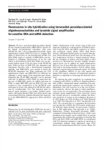
FIG. 1. Two FISH images used in dot counting taken at the same FOV but at different planes: (a) in-focus image and (b) out-of-focus image.

mechanism has a number of problems. First, automatic acquisition is dependent upon finding the sharpest image. It can fail, however, if the mechanism focuses on a source of noise such as debris or background fluorescence or if the FOV is empty (4,5). Therefore, subsequent manual inspection for discarding such images is sometimes inevitable. Second, even if the sharpest image is found, it only represents a section of a 3D image. Signals in other sections that are above or below that section do not participate in the analysis. Third, auto-focusing is time consuming. It takes almost 10 s to complete auto-focusing of one FOV (5), which is 50 –75% of the total time needed to analyze that FOV. Finally, research (5) shows that autofocusing contributes about 3% of the total 11% error rate of the analysis. As an alternative to the use of an auto-focusing mechanism, we suggest basing FISH dot counting on a neural network (NN) classifier that discriminates between in and out-of-focus images taken at different focal planes of the same FOV (Fig. 1). Images at different focal planes of a specific FOV compose a stack of images that represents this FOV. Each stack image is analyzed and its signals are classified by the NN as valid data or artifacts, which are the result of out of focusing. Following the discrimination of valid signals and artifacts in each stack image, the image that does not contain artifacts is selected as the in-focus image to represent the stack (FOV), whereas the other stack out-of-focus images may be rejected. The procedure is then repeated for other FOVs until the entire slide is covered or the required number of (in-focus) images (or nuclei) are collected (Fig. 2). Proportion estimation of the number of cells having specific numbers of signals can then be performed using these images as in auto-focusing– based dot counting methods (3,5). The suggested method overcomes most of the shortcomings of auto-focusing because it does not necessarily depend on a single image but on a stack of images. Moreover, the method shortens

FIG. 2. A flow chart of a dot counting system based on a classifier, instead of an auto-focusing mechanism, that discriminates between in and out-of-focus images.

89

AUTOMATIC SIGNAL CLASSIFICATION

the length of image acquisition, as stack images are captured coarsely without the necessity of finding the exact location of the in-focus image. Combined with multispectral analysis, the suggested methodology also shortens the length of image analysis. Finally, the proposed method enables flexibility because the NN classifier can be integrated into any existing dot counting system. It replaces the auto-focusing mechanism and can be replaced by any other classifier. However, as the system is required to classify valid signals and artifacts, its ability to discriminate between focused and unfocused signals should be more accurate than that of the discriminating element of a system employing an auto-focusing mechanism. This is because the latter encounters only valid signals. Therefore, the proposed system depends on two components: a highly accurate classifier to distinguish between valid and artifact signal data and well-discriminating multifeature signal representation. We have previously investigated (6) the second component of feature representation for FISH signals. In the present study, we examine the use of a classifier to discriminate between valid and artifact signals. Focused signals are valid signals and they are classified as “reals.” Unfocused signals and signals created by background fluorescence or due to overlap between different fluorophores located in different focal planes are classified as “artifacts.” A two-layer perceptron NN trained using large numbers of examples of these two classes is employed for the classification. MATERIALS AND METHODS Slide Preparation The interphase nuclei preparations from amniotic fluid were made using the method of Klinger et al. (7) with minor modifications. Amniotic fluid (1–2 ml) was centrifuged and the cell pellet washed in phosphate-buffered saline (PBS) warmed to 37°C. The cells were resuspended in 75 mM KCl and placed directly on slides coated with APES (Sigma, St. Louis, MO) and incubated at 37°C for 15 min. Evaporation of PBS was compensated with filtered distilled water. Excess fluid was carefully removed and replaced with 100 ml of 3% Carnoys fixative and 70% 75 mM KCl at room temperature for 5 min. The excess fluid was carefully removed and five drops of fresh fixative were dropped on the cell area. Slides were briefly dried on a 60°C hotplate. They were either used immediately for hybridization or dehydrated through an alcohol series and stored at ⫺20°C until required. Hybridization Target areas were marked on the slides using a diamond-tipped scribe. Target DNA was denatured by immersing in 70% formamide:30% 2 ⫻ SSC at 73°C for 5 min. Probe mix (10 ␮l) containing spectrum orange LSI 21 and spectrum green LSI 13 (Vysis, UK) was applied to the target area and a coverslip placed over the probe solution. Coverslips were sealed using rubber cement and slides

were placed in a prewarmed humidified container in a 37°C incubator for 16 h. Coverslips were removed and slides washed in 0.4 ⫻ SSC/0.3% NP-40 solution at 73°C for 2 min. Slides were then placed in 2 ⫻ SSC/0.1% NP-40 solution at room temperature for 1 min. When completely dried, 10 ␮l of DAPI II counterstain (Vysis) was applied to the target area and sealed under a coverslip. Instrumentation and Screening Procedure Slides were screened under a Zeiss axioplan epifluorescence microscope using a Zeiss ⫻100 objective. Signals were viewed using a Vysis DAPI/green/orange triple band pass filter set and images were acquired using a CCD camera (Photometrics CH250/A) and SmartCapture software (Vysis). Red and green signals, corresponding to chromosomes 21 and 13, respectively, were seen on blue DAPI-stained nuclei. Because acquiring stacks of images for the different FOVs is a relatively demanding task, we use a simpler procedure in this study. Slides were scanned by starting in the upper left corner of the coverslip and moving from top to bottom. The focus and color ratios were adjusted for the first captured image from each slide. Those values were kept for all the following images from that particular slide. Images were captured by stopping at random intervals along the slide. Utilizing this acquisition procedure and assuming uniform distribution of signals along the Z-axis, we captured an arbitrary mix of in and out-of-focus images without literally collecting stacks of images. For evaluating the classification of focused and unfocused signals, this procedure provides the desired images cheaply and quickly. However, for testing the entire system in dot counting (Fig. 2), stacks of images will be acquired. A total of 400 in and out-of-focus images were collected from five slides, stored in TIFF (Tagged Image File Format), and used in the signal classification experiments. IMAGE ANALYSIS Multispectral Analysis Multiple probes, labeled by different fluorophores, are often used in conjunction in FISH preparation. For example, in our study, chromosomes 13 and 21 are indicated by green and red signals, respectively, and the nuclei are colored in blue (Fig. 1). The position in the image and the characteristics of each of these fluorophores have significant meaning to the researcher or clinician. Nevertheless, in most of the previous research of automatic FISH image analysis (4,5), color information is converted into graylevel scale. FISH image analysis is then based on intensity and not on color information, which is lost in the process. However, much of the difficulties encountered during the analysis of intensity images can be avoided if color information is maintained and used. This is especially true for nucleus and signal segmentation. Many user-defined thresholds and heuristics are needed to segment signals from nuclei and nuclei from background when intensitybased analysis is employed. In this study, color is kept and specified by the RGB (red, green, blue) format, in which each image pixel is

90

LERNER ET AL.

represented by the normalized red, green, and blue brightness values. DAPI nuclei are analyzed in the blue channel of the RGB image, whereas red (spectrum orange; chromosome 21) and green (spectrum green; chromosome 13) signals are analyzed separately in the red and green channels, respectively. Multispectral image analysis does not only facilitate preprocessing and segmentation (3), it also yields hue-based features, which are found very efficient for FISH signal representation and classification (6). Furthermore, it allows the analysis of multiple probes. Color Image Segmentation Special multistage (usually TopHat-based) procedures that rely on heuristically derived thresholds and parameters are conventionally applied to the intensity image in order to segment nuclei and signals (4,5). Color image segmentation, however, avoids the use of these procedures. It is performed separately on each of the three different channels of the RGB image using global thresholds. Finding optimal global thresholds in the RGB image is almost trivial compared with thresholding an intensity image because the channels contain no background and only blue (red, green) objects are found in the blue (red, green) channel. Also, for these reasons, moderate changes in the threshold values barely affect the overall accuracy of image analysis. In this study, threshold values of 0.5 and 0.8 of the maximum channel intensity are suitable for the segmentation of signals and nuclei, respectively. In addition, when performing the analysis, the red and green channels of the color image can be represented by sparse matrices (note that the area of a typical signal of 10 pixels is less than 0.01% of a typical image area, i.e., 400 ⫻ 400 pixels2). Therefore, special algorithms for sparse matrices can be exploited to enable fast performance of multispectral analysis, which cannot be exploited while analyzing the full matrices associated with the intensity image. Following thresholding, noise reduction, boundary smoothing of the nuclei by morphological operations, and spatiospectral correlation between nuclei and signals are implemented to complete segmentation of the nuclei and signals. Signal Feature Measurement Several features are measured for each of the segmented signals. Features include area (a size measure), eccentricity (a shape measure), total and average channel intensities (intensity measures), and intensity standard deviation (texture measure). All but the last feature have been suggested previously (4) to represent signals, albeit measured using the intensity image. We also measure the maximum and average hue (color measures) as they are more appropriate for signal discrimination than RGB-based features (6). Hue features can be measured only if color information is kept. The RGB image is then converted into the HSI (hue, saturation, intensity) format. Several features are representative for signal classification when evaluated using scatter plots, probability density functions, a class separability criterion, and the probability of misclassification (6). Among these features are

the area, average channel intensity, and average hue of the signals. These three features are employed here to represent the segmented signals to the classifier. SIGNAL CLASSIFICATION The main purpose of this study is to investigate the feasibility of automatic signal classification in in and outof-focus FISH images. Although the application of the research is to dot counting, we are not interested for the moment in estimating the proportions of cells having specific numbers of signals, but rather in the ability to accurately distinguish between valid signals (reals) and artifacts. This ability forms the basis of the proposed dot counter (Fig. 2). In the common procedure of automatic dot counting, signals whose relative intensity and either total intensity (4) or area (5) are in specific intervals are classified as reals, while other signals are rejected. The interval is defined by the minimum and maximum values of the features as measured on a training set composed of valid signals. Signals of out-of-focus images are manually excluded. Such a strategy is not appropriate for the methodology we are suggesting here for a number of reasons. First, even the best one (or two) discriminative features would fail to provide sufficient classification accuracy when signals have to be classified as reals or artifacts of several fluorophores (6). Dealing with a complex multiclass classification problem usually requires the use of multivariate patterns. Second, as the training set includes only valid signals, the classifier is limited in its ability to model artifacts. Therefore, it may miss the correct decision boundaries of the artifact classes, which yield the minimum probability of misclassification. Third, as the decision boundaries are determined by the minimum and maximum feature values, they are only a rough approximation of the real decision boundaries determined by feature values of the entire training data set. Moreover, boundaries based on extremes are sensitive to outliers. In the presence of outliers, the probability density functions of valid signals and artifacts may overlap to a greater extent and the probability of misclassification of the classifier may then be increased. Therefore, the classification procedure proposed here is as follows. 3D patterns of signals [or higher-dimensional patterns as reported by Lerner et al. (6)], which are based on the signal area, average channel intensity, and average hue are examined. The patterns (representing the spectrum orange and spectrum green probes) are classified into four classes: real red, artifact red, real green, and artifact green. Within the artifact classes we expect to find unfocused and overlap signals, and signals that are the result of background fluorescence. These signals will have patterns with different values of features than those of valid signals, and hence will be classified as artifacts (compare Figs. 1a and 1b). Labels for the patterns, belonging to one of the four classes, are needed to train and evaluate the classifier. They are obtained by a cytogeneticist using a custom-built graphical environment for labeling FISH images (8).

AUTOMATIC SIGNAL CLASSIFICATION

91

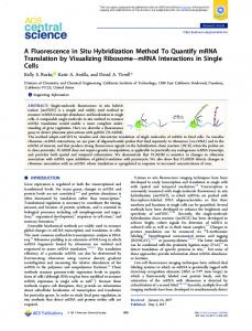
FIG. 3. Classification accuracy of the (a) monolithic and (b) combined strategies for increasing numbers of hidden units (notice the different scales along the two y-axes).

Following the normalization of the features to zero mean and unit variance, patterns of signals extracted from all the images are divided randomly into training and test sets and classification into one of the four classes is implemented using cross-validation. In the variant of crossvalidation technique used in this study, the data are partitioned into five equal parts. Four fifths of the data are used for training and the remaining one fifth is kept for the test. The experiment is repeated five times. Each time, another four fifths (one fifth) of the data are employed for the training (test). Classification accuracy is then averaged over the five experiments (CV-5). The classifier is a twolayer perceptron NN trained by the scaled conjugate gradient algorithm (detailed descriptions of NNs and learning algorithms for NNs can be found in ref. 9, Chapters 4 and 7, respectively). Classification is based on the approximation of the two-layer perceptron outputs to the a posteriori probabilities for the classes. A validation set, which is drawn from the training set, assures that the classifier is not overtrained. It also allows the selection of a minimal network configuration based on only a few hidden units. Both factors ensure rapid training and improved generalization. Three classification strategies are examined here. In the first, called the monolithic strategy, patterns are classified into the four classes using a single NN. In the second, termed the independent strategy, patterns are classified into red and green classes using the color network and independently by a second network, the real network, into reals and artifacts. Classification of a pattern into one of the four classes is achieved by a common decision of both networks. In the third strategy, called the combined, patterns are first classified into red and green classes using

the color network. Then, based on the results of this network, they are classified by two other networks, the real-red network and the real-green network, into reals and artifacts of the two colors. EXPERIMENTS AND RESULTS We established a database of 400 in and out-of-focus FISH images captured from five slides. Following nuclei segmentation, the system identified 944 objects within these images as nuclei, of which 613 also contained signals (the remaining 331 objects are unfocused nuclei that do not contain signals). Following signal segmentation, 3,144 objects within the above nuclei were identified as signals and features were measured for them. Based on labels provided by expert inspection, 1,145 of the signals were considered as reals (among them 551 were red) and 1,999 as artifacts (among them 1,224 were red). First, experiments to find suitable configurations for the NNs of each of the three strategies were performed. Input and output dimensions for the networks were set by the feature space dimension and the number of classes, respectively. The number of hidden units was determined such that the network had the highest generalization capability. This was achieved by evaluating networks of different numbers of hidden units on an independent validation set (9) drawn from the training set. The network that had the lowest error measured on the validation set was selected for training. Figure 3 shows the results of experiments with the monolithic and the combined strategies for determining the number of hidden units for each network, and therefore their configurations. Table 1 gives the configurations selected for the networks of each of the classification strategies. The number of hidden units is

92

LERNER ET AL.

Table 1 Configurations and Classification Accuracies on the Training and Test Sets of the Three Classification Strategies: Monolithic, Independent, and Combined*

Configuration Training (%) Test (%)

Monolithic

Real

Color

Independent

Combined

3:27:4 84.0 82.9

3:13:1 87.5 87.3

3:13:1 96.4 95.7

3:13:1 84.1 83.3

3:13:1 87.9 87.1

*Configurations are specified by the numbers of units in each layer of the NN (input:hidden:output). Results for both the real and the color networks are needed to obtain the overall classification accuracies of the independent and combined strategies. Signals are represented by their area, average channel intensity, and average hue. (The slight deviations in classification accuracy of the combined classifier compared with Figure 3b are attributed to the different experiments using random classifier initializations and randomly selected data sets.)

selected by the highest classification accuracy on the validation set. Finally, training of each of the networks was continued for 100 epochs (presentations of the entire training set). The results were averaged for each network over three random initializations. The classification accuracies of the monolithic strategy, using its optimal configuration, were 84.0% and 82.9% for the training and test sets, respectively (Table 1). We also examined the sensitivity of the classification accuracy of this strategy against the sample size by repeating the experiment for training sets of different sizes. The size of the training set was increased from 10% to 90% of the data, where the same unseen 10% of the data was used for the test. The results in Figure 4 demonstrate that the classification accuracy on the test set follows, as expected, the increase of the training sample size until its maximum level. However, the classification accuracy on the training set has a minimum. The explanation is that for a very small sample size, training is very simple and classification of a few training patterns can be very accurate. It is, however, more difficult to maintain this accuracy as the sample size

FIG. 4. Classification accuracy of the monolithic strategy for increasing sample sizes.

increases and more variants of the training patterns are added. The classification accuracy decreases until it reaches a minimum for a critical mass of learned patterns. After this point, as sample size continues to grow, the additional patterns are not so different from those of the critical mass. Thus, learning of the patterns of the (extended) critical mass is intensified. At the same time, the fraction of misclassified patterns becomes lower. The result of both trends is toward the improvement of the classification accuracy on the training set as shown in Figure 4. Experiments with the other two strategies, the independent and the combined, reveal that these strategies can improve the classification accuracy of the monolithic strategy by 0.4% (to 83.3%) and 4.2% (to 87.1%), respectively, when tested on unseen data (Table 1). Table 1 also demonstrates that classification of signals into their colors is more accurate than that of signals into reals and artifacts. Finally, the combined strategy, when tested using an extended feature set (6), has achieved classification accuracy of 89.2%. DISCUSSION In dot counting, the application of an auto-focusing mechanism to the acquisition of FISH images usually enables the analysis of nuclei and signals from focused images. However, the distributions of signals within a nucleus and nuclei within a specimen are uniform. Because the auto-focusing mechanism can focus on debris and background fluorescence, signals are often left unfocused. Consequently, missing images are analyzed and dot counting suffers from errors. Moreover, errors in the focus position also cause errors and high variance of the values of the features that represent the signals (4). The result of all these errors is enhanced significantly as the number of probes increases. In addition, auto-focusing requires a large fraction of the analysis period: around 50 –75% of the total time needed for analyzing a specific FOV is devoted to auto-focusing (5). In summary, auto-focusing is a long and critical step of FISH image analysis. Failure of autofocusing will undermine the whole analysis and lead to unreliable results (3,5).

93

AUTOMATIC SIGNAL CLASSIFICATION

An alternative methodology is proposed in this study. It is based on the employment of a NN classifier to distinguish between in and out-of-focus images. Signals of images composing a stack are classified as valid data or artifacts due to out of focusing. The stack image that contains no artifacts is selected as the in-focus image to represent this stack (FOV). In-focus images collected and analyzed from the entire slide (or sample) can be exploited for dot count proportion estimation of the specimen. Processing of color in FISH images makes nucleus and signal segmentation, as well as signal classification, easier and less sensitive to noise. It reduces the employment of user-defined thresholds and prevents the excessive application of heuristics, both of which are necessary in intensity-based image analysis. Furthermore, analyzing the sparse matrices associated with FISH multispectral images is much faster than that of the full matrices associated with FISH intensity images. Compared with the two common imaging methods, single excitation (SE) and dual excitation (DE) (5), multispectral image analysis combines the advantages of both methods. It allows separate processing of signals of different fluorophores while capturing only one image. It also suggests an improvement to current methods (4,5) because it is suitable for use with more than two fluorophores. Finally, multispectral image analysis enables richer and more discriminative representation of signals of several fluorophores, yielding an accurate signal classification. Classification of multiprobe valid and artifact signals in in and out-of-focus images is a more demanding task than the detection of single-probe valid signals in in-focus images. For the former task, we suggest a methodology based on 3D multispectral image analysis and a trainable, nonlinear, multiclass classifier such as a NN. This novel methodology when applied to dot counting has several advantages compared with that employing intensity-based image analysis and an auto-focusing mechanism. First, the system is not limited to signals of one probe. Second, image acquisition and analysis using the new methodology are performed more quickly and are less dependent on heuristics. This is because the system avoids auto-focusing and makes use of the color rather than the intensity image. Third, the inevitable out-of-focus signals do not undermine dot counting as in an auto-focusing– based system. These signals define the artifact classes required for training the classifier (off-line) to reject out-of-focus images during dot counting. Fourth, the proposed methodology permits the performance of 3D dot counting, as signals captured in different focal planes of the same FOV can be analyzed commonly. In addition, the NN classifier can be incorporated into any existing dot counting system, as it only replaces the auto-focusing mechanism, and it can also be replaced by non-NN classification paradigms. NN-based hierarchical classification strategies examined in this study decreased the classification complexity. They shortened the training session and improved the accuracy compared with a monolithic NN strategy. Test signals of two fluorophores extracted from nuclei of in and out-offocus images were classified as valid signals and artifacts

with an accuracy of 87.1% [or 89.2% for other feature sets (6)]. Furthermore, classification of test signals was accomplished instantaneously because it only required the multiplication of 3D feature vectors representing the signals with two (monolithic strategy), four (independent strategy), or six (combined strategy) small weight matrices of the previously trained NN classifier. In summary, the suggested methodology, based on multispectral image analysis and signal classification, is an accurate and efficient screening mechanism for obtaining in-focus images in dot counting. CURRENT AND FUTURE RESEARCH Current research has two aims. The first aim is to improve the performance of signal classification by increasing its accuracy while keeping its simplicity. Recent research (10) has stepped on this track. The second aim is the application of the suggested system to stacks of images, and thereby the accomplishment of the complete classifier-based multispectral dot counting system (Fig. 2). Stacks of images have been already collected for this purpose. Proportion estimation of cells having different numbers of signals (0, 1, 2, . . .) can then be performed and the performance (accuracy and speed) of the system can be compared with that of auto-focusing– based dot counters. The suggested dot counting method, if found accurate in performing proportion estimation as its counterpart, will be advantageous due to the benefits demonstrated in this study. ACKNOWLEDGMENTS The authors thank the anonymous referees for their most valuable comments. LITERATURE CITED 1. Tanke HJ, Florijn RJ, Wiegant J, Raap AK, Vrolijk J. CCD microscopy and image analysis of cells and chromosomes stained by fluorescence in situ hybridization. Histochem J 1995;27:4 –14. 2. Carothers AD. Counting, measuring, and mapping in FISH-labelled cells: sample size considerations and implications for automation. Cytometry 1994;16:298 –304. 3. Castleman KR, White BS. Dot count proportion estimation in FISH specimens. Bioimaging 1995;3:88 –93. 4. Netten H, van Vliet LJ, Vrolijk H, Sloos WCR, Tanke HJ, Young IT. Fluorescent dot counting in interphase cell nuclei. Bioimaging 1996; 4:93–106. 5. Netten H, Young IT, van Vliet LJ, Tanke HJ, Vroljik H, Sloos WCR. FISH and chips: automation of fluorescent dot counting in interphase cell nuclei. Cytometry 1997;28:1–10. 6. Lerner B, Clocksin WF, Dhanjal S, Hulte´n MA, Bishop CM. Feature representation for the automatic analysis of fluorescence in-situ hybridization images. IEEE Trans. on Systems, Man and Cybernetics, accepted. 7. Klinger K, Landes G, Shook D, Harvey R, Lopez L, Locke P, Lerner T, Osathanondh R, Leverone B, Houseal T, Pavelka K, Dackowski W. Rapid detection of chromosome aneuploidies in uncultured amniocytes by using fluorescence in situ hybridisation (FISH). Am J Hum Genet 1992;51:55– 65. 8. Lerner B, Dhanjal S, Hulte´n MA. GELFISH: graphical environment for labelling FISH images. J Microscopy, accepted. 9. Bishop CM. Neural networks for pattern recognition. Oxford: Clarendon Press; 1995. 10. Lerner B. A Bayesian methodology and probability density estimation for fluorescence in-situ hybridization signal classification. Technical Report 474, Computer Laboratory, University of Cambridge, October 1999.