corresponding locations in the images has two stages. The first is ...... select candidates that are deemed globally optimal to achieve a final 1:1 feature mapping.
Automatically Synthesising Virtual Viewpoints by Trinocular Image Interpolation — Detailed Report Stephen Pollard, Sean Hayes, Maurizio Pilu, Adele Lorusso Digital Media Department HP Laboratories Bristol HPL-97-166 December, 1997
image processing, image based rendering, computer graphics, stereo matching
We present a computationally simple and fully automatic method for creating virtual views of a scene by interpolating between sets of images obtained from different viewpoints. The technique is intended to give an immersive experience and a sense of viewing a real environment. The method uses correspondence points identified in the primary images. The matching of corresponding locations in the images has two stages. The first is based on ‘corner points’ and is used to extract the epipolar geometry that relates the images, then a second stage of edge matching recovers a more complete set of correspondences. These edge correspondences are then interpolated and used in an efficient morphing algorithm that operates one scanline at a time to perform image synthesis.
Internal Accession Date Only
Copyright Hewlett-Packard Company 1997
Table of Contents 1.
INTRODUCTION ......................................................................................................................... 3
2.
GEOMETRY................................................................................................................................. 5
3.
SYSTEM ARCHITECTURE...................................................................................................... 10 3.1 3.2
CAPTURE ................................................................................................................................... 10 RENDERING ............................................................................................................................... 11
4.
IMAGE CAPTURE ..................................................................................................................... 12
5.
CAPTURE PROCESSING.......................................................................................................... 14 5.1 EPIPOLAR GEOMETRY ESTIMATION ............................................................................................. 14 5.1.1 Establishing feature correspondence .............................................................................. 14 5.1.2 Fitting the Epipolar Geometry ......................................................................................... 16 5.2 EDGE DETECTION AND LINKING ................................................................................................. 17 5.3 EDGE MATCHING ....................................................................................................................... 18 5.3.1 Binocular Row Matching ................................................................................................. 19 5.3.2 Dynamic Programming.................................................................................................... 21 5.3.3 Weak Trinocular Consistency .......................................................................................... 23 5.3.4 Matching Edge Strings..................................................................................................... 26
6.
RENDERING .............................................................................................................................. 28 6.1
RASTER RENDERING................................................................................................................... 31
7.
VIOLATING MONOTONICITY............................................................................................... 35
8.
DISCUSSION AND CONCLUSIONS......................................................................................... 36
9.
REFERENCES ............................................................................................................................ 37
1
Index of Figures Figure 1: Parallel Binocular Cameras............................................................................... 5 Figure 2: Parallel Trinocular Cameras.............................................................................. 6 Figure 3: General Trinocular Geometry ........................................................................... 8 Figure 4: Immersive Video Processing........................................................................... 10 Figure 5: Video Capture Hardware................................................................................ 12 Figure 6 Edge String Representation ............................................................................. 18 Figure 7: Defining the Epipolar Range........................................................................... 20 Figure 8: Defining Epipolar Pairs................................................................................... 20 Figure 9: Epipolar Intersection ...................................................................................... 21 Figure 10: Dynamic Programming Table........................................................................ 22 Figure 11: The Weak Trinocular Matching Constraint ................................................... 24 Figure 12: Trinocular Similarity Measure....................................................................... 25 Figure 13: Edge String Consistency............................................................................... 27 Figure 14: Interpolating Matched Edge Strings.............................................................. 28 Figure 15: Edge Interpolation........................................................................................ 29 Figure 16: Rendering Architecture................................................................................. 29 Figure 17: Raster Intersection ....................................................................................... 29 Figure 18: Raster Intersection Table.............................................................................. 30 Figure 19: Raster Rendering.......................................................................................... 31 Figure 20: Pixel Rendering ............................................................................................ 32 Figure 21: Intensity Interpolation .................................................................................. 32 Figure 22: Synthesised Images....................................................................................... 33 Figure 23: Improved Rendering..................................................................................... 35
2
1. Introduction The worlds of 3D computer graphics and digital video processing are rapidly converging. Separate traditional domains such as CAD, virtual environments and interactive 3D games on the one hand and video conferencing, video post-production and non-linear editing on the other are giving way to hybrid approaches that combine technologies [0, 2, 3, 4]. The emergence of standard graphic and video enabled computing/entertainment platforms coupled with the growth of high bandwidth communications infrastructure will only increase this trend toward interactive digital media capabilities in both the home and office computing appliances. A growing number of researchers are exploring the generation of static and temporally varying immersive scenes using real world image data alone. One approach is to capture all viewpoints at a single point and use these as an environment map [5, 6, 7] to be applied as a texture on some imaging surface. Particular viewpoints can be generated by projecting the texture onto the imaging plane corresponding to the users current view. Environment maps can be obtained as panoramas composed from multiple images and composted as cylindrical projections [8] or based upon lens and/or mirrors designed for all round capture onto a single imaging array [9, 10]. A number of commercial systems, including QTVR (Apple Computer), PanoramIX (IBM), IPIX (Interactive Picture Corporation) and Realspace (Live Picture) have been developed. Methods for morphing between environment maps have also been proposed [11, 12]. Good overviews of image mosaic generation to capture virtual environments are available in [13, 14, 15]. It is possible to go beyond the exploration of 2D worlds (where the viewer is constrained to a single, or predetermined set of discrete, locations in the 3D environment) by directly representing the light field in the vicinity of an object [16, 17]. The light field in regions of free space is a 4D function of radiance against position (2 parameters; as all points along a single light ray have the same radiance) and direction (2 parameters). The light field can be constructed from the dense set of images captured over a planar grid (an image of images). However it proves difficult to capture in practice (precise calibration and camera positioning are required) and has onerous memory requirements. Another approach to viewpoint synthesis is to recover a dense 3D model or depth map from multiple discrete images or a video sequences and to employ standard texture mapping technique to view that surface from an alternative viewpoint [18, 19, 20, 21]. This approach also requires precise calibration, especially if the viewer is to be allowed to transform the object far from the original viewpoints. Furthermore, occlusion proves a particular problem for the construction of a dense depth map. Depth estimates will be inaccurate along depth discontinuities and absent altogether in extended occluded regions. A frequently employed approach is to compensate for occlusion by combining depth estimates from a large number of image pairs.
3
The work described here follows a simple approach. It uses image morphing techniques to synthesise viewpoints between a small number of original images. The approach owes much to the work of Seitz and Dyer [22, 23] in particular the implementation is an extension of that developed in [22]; the method is automatic and relies on edge based stereo processing to identify a set of sparse edge correspondences between the original images. New views are constructed by linearly interpolating the matched edges and efficiently rendering individual rasters on the basis of the interpolated edges that cross them. This approach gives surprisingly high quality image reconstruction over the viewing regions between original camera positions provided that their camera geometry is not too dramatic. The approach has a number of advantages over alternative schemes. It does not require accurate camera calibration; sufficient information for edge matching can be recovered from the images themselves. The sparse edge data has only a low overhead over the original images. The raster based rendering algorithm gives the impression of surfaces sliding behind one another at occlusions and is robust to missing edge data. The method leads naturally to the development of an immersive video media type in which multiple video tracks are augmented with a morphing track to allow the viewer to alter their viewpoint with respect to the video sequence in real time.
4
2. Geometry P
I0 p0
I0.5
f0
(p0+p 1)/2
C0 f0.5 p1
I1
C0.5 f1 C1
Figure 1: Parallel Binocular Cameras Consider the parallel camera geometry shown in Figure 1 (recreated from [23]). It shows a pair of cameras with optical centres C0 and C1 displaced in a direction orthogonal to the common direction of the principal axes. Note that the focal lengths of the cameras need not be preserved. In such cases linear interpolation of the 2 images, I0 and I1 is shape preserving and results in viewpoints along the line C0 C1 joining the optical centres of the 2 cameras. For example the image, I0.5, of a third parallel camera at the mid-point C0.5 with the mean focal length is given by the mean projection of image locations in the 2 images.
5
C2
f2 p2 P
C0
f0 p0
p1 C1
f1
Figure 2: Parallel Trinocular Cameras Here we extend this approach to 3 cameras as shown in Figure 2. Again the principal axes of each camera are parallel, orthogonal to the plane that passes through the 3 optic centres and all the image planes have the same orientation. Choosing the origin of the co-ordinate frame at C0 aligned with the image plane and principal axis of the first camera then the projection of a point P in the world is given by
[x
0
y0
f0 Z = T0 P = 0 0
]
0 f0 0
X 0 0 Y 0 0 Z 1 0 1
in image 1
[x
1
y1
f1 Z ] = T1P = 0 0
0 f1 0
in image 2, and
6
X 0 − f 1C1x Y 0 − f 1C1y Z 1 0 1
[x
y2
2
f2 Z = T2 P = 0 0
]
0 f2 0
X 0 − f 2 C2 x Y 0 − f 2 C2 y Z 1 0 1
in image 3. Linear
[
interpolation
p 0 = x2 Z
]
amongst
[
p 0 = x0 Z
]
y0 Z ,
[
p 1 = x1 Z
]
y1 Z and
y 2 Z yields (1 − β )((1 − α )p 0 + αp 1 ) + βp 2 = (1 − β )((1 − α ) =
T0 P T1 P T2 P +α )+β Z Z Z
Ts P Z
where
Ts = (1 − β )((1 − α )T0 + αT1 ) + βT2 image interpolation therefore produces a new view whose projection matrix is a linear interpolation of the original 3. Hence interpolating images from parallel cameras produces the illusion of moving the camera on the plane through the optical centres. More generally this approach applies wherever the 3rd row of the three transformation matrices is constant.
7
Figure 3: General Trinocular Geometry
Let us assume that the cameras can be approximated with an affine model (see, e.g., [24]). Let us refer to Figure 3 and consider a point P=[X,Y,Z,1] in the space imaged by three affine, uncalibrated cameras defined by affine projection matrices A0, A1 and A2 scaled such that Ai(3,4) =1 (i=0..2). The projections of a point P onto the image planes of the cameras are given by p0=[x0 y0 1]T=A0P, p1=[x1 y1 1]T=A1P and p2=[x2 y2 1]T=A2P. Let the interpolation of these three points in image plane coordinates be given by: ps= (1 − β )(( 1 − α ) p 0 + α p 1 ) + β p 2 = (1 − β )(( 1 − α ) A 0 P + α A 1 P ) + β A 2 P = A s P
where A s = (1 − β )((1 − α ) A 0 + αA 1 ) + βA 2 . Thus interpolation in the image plane produces the same effect as having an another affine camera As.
8
But what does this interpolated affine matrix look like? Ullman and Basri [25]show the conditions under which linearly interpolating orthographic views produces other veridical views. Chen and Williams [1] used interpolation between range data to synthesise intermediate views and again found that valid views are produced only under some circumstances. Since, as we shall see later, our approach does not explicitly use parallel camera rectification as in, we have to understand what an interpolated affine camera matrix represents. An affine transformation can be seen as a parametric mapping from ℜ3 → ℜ2 A i = A i (v ) = A i (θ , ϑ ,ψ , t x , t y , t z , S , S x , S y )
function of the camera reference frame orientation and position, plus a shearing and two scaling components, respectively. Now, since the tranformation is linear in translation, scaling and shearing, if no rotation between the cameras A0 , A1 and A2 is involved, As represents a perfectly valid new viewpoint V. On the other hand, when rotation is involved this is no longer true. However, provided the relative rotations cameras between the cameras are small, there is a near-linear relationship between changes in the elements of the affine matrices and changes in the gaze angles. Hence, under these conditions in general we can write: As ≈ A0 ((1 − fβ (β ))((1 − fα (α ))v0 + fα (α )v1 ) + fβ (β )v2 )
where f α (α ) f β (β ) are non-linear functions of α and β . Thus the synthesised viewpoint, neglecting second order effects, simulates the camera being on the hyper-plane through v0, v1 and v2. In summary our approach is to use linear image interpolation to approximate the change in viewing position amongst an initial set of imaging locations. This does not require knowledge (through calibration or otherwise) of the actual locations of the cameras, provided they have sufficiently similar orientations and the camera baseline is reasonably small with respect to viewing distance (i.e. more than 5::1).
9
3. System Architecture The overall system architecture is illustrated in Figure 4. It allows either two or three image sources (still images, or corresponding frames from video streams) captured from spatially displaced locations to be processed. There are 2 main components to the processing architecture: • capture: up to the extraction of strings of matched edge points. • rendering: using the matched edge data to morph the images. While it is possible for both capture and rendering to be performed in real time, capture is currently the more computationally demanding part of the problem and can for some applications be performed off line. In any case, some form of image and edge compression can be used between capture and rendering to reduce bandwidth for transmission, broadcast or long term storage
Image Capture
Image Capture
Image Capture
Edge Detection
Edge Detection
Edge Detection
Edge Linking
Edge Linking
Edge Linking
Edge Matching
Capture potential compression for network delivery or storage
Rendering Edge Interpolation
3.1 Capture Raster The first requirement is the Rendering simultaneous capture of two or more views of a given scene. Then, using some standard image processing Figure 4: Immersive Video Processing techniques on the captured images, an edge map is determined for each view. Using the edge maps and the original images, stereo matching is performed to determine which edges in one image correspond to which edges in the remaining images. In order to perform this stereo matching the epipolar geometry that relates the cameras is required [26]. Stereo matching is somewhat simplified in the context of three or more (even weakly) calibrated cameras [27, 28 and 29]. In general each new camera provides additional 10
constraints on the stereo matching problem. While edge matching is under-constrained for two views, the addition of a third view allows potential matches identified between the first two images to be verified. Our edge matching scheme is able to work with two images but is more robust when working with three.
3.2 Rendering The rendering stage is essentially a two phase process, firstly a new ‘line sketch’ is generated, which is an interpolated version of the captured edge maps, then a scan line rasterisation is used that ‘colours in’ the sketch using re-sampling and image morphing of the original image data.
11
4. Image Capture The actual details of the physical image capture are highly specific to the capture devices and computer architectures involved. We have experimented with colour digital still cameras, genlocked monochrome video sources digitised directly on a PC and multiple digital video camcorders. Since one aim of the work was to create an immersive video effect by interpolating views from multiple video sources, one demanding problem was the physical capture of three simultaneous videos to disk at a reasonable frame rate. Although simple in principle, the limitations of affordable hardware give rise to a number of technical problems. The problems we encountered were notably: 1. Very few (and expensive) video grabbers allow the capture and store three RGB images simultaneously, and those which do rely on theoretical PCI-bus bandwidth, which is rarely attainable in practise. 2. Compression methods are not yet the norm for video grabbers, so data was kept in raw format, which only served to increase the bandwidth limitations. 3. The PC memory-to-disk transfer rate is practically 5-7 Mb/s even on the most up-todate machines, which is utterly inadequate for frame-rate video storage. Although these limitations could have been overcome by the application of expensive custom hardware, we opted instead for a trade-off that allowed us to keep costs dramatically down while nonetheless substantially achieving our aims. The figure below shows the diagram of the capture set-up we have used.
Camera #1 genlocks camera #2 and camera #3
Camera #1 VIS TA
sync Camera #2
Matrox Meteor RGB
VISTA
sync Camera #3 VIS TA
Figure 5: Video Capture Hardware By limiting the capture to monochromatic video each source could be captured to one channel of a cheap RGB capture board (the METEOR-RGB in this case). The cameras are genlocked, that is one synchronises the other two, which are configured in external sync
12
mode. The cameras used, (VISTA 230), do not have automatic gain control and were fitted with 6mm lenses witch give a field of view of about 60 degrees. A further benefit of restricting the system to monochromatic channels is the lower bandwidth when transferring data to disk. A CCIR image of 576x768x8 pixels is about 350 Kbytes and three of them make about 1 Mbytes of data per frame, which allows us to capture and store three video streams at 5-7 frames per second. Were we dealing with colour images, say PAL, we would have had three times as much data (if not four due to 32 bit word alignment) and so the storable frame-rate would have dropped to an unacceptable 1.2-1.7 frames/s. In order to bypass the disk bandwidth problem, we also tried storing all frames in system memory and then saving them to disk at the end. Using 128 Mbytes RAM enabled the capture of about 4 seconds of videos at full frame rate.
13
5. Capture Processing Capture processing involves: • • •
epipolar geometry recovery, to determine the model that relates the cameras. edge detection and linking: the identification of pixel locations that represent the locus of edges in the image and their subsequent grouping into extended edge strings. edge matching: the identification of corresponding edge points between the image streams.
5.1 Epipolar Geometry Estimation The epipolar geometry [26] is the model that relates two images taken from either a single moving camera or a pair of cameras. This needs to be determined only when the cameras move with respect to each other, so for two video streams from static cameras this expensive step could be performed once at set-up, and then reused for each frame. For any feature in one image, captured with a pinhole camera, the corresponding feature in the other image will lie on an epipolar line. Historically epipolar geometry was used for calibrated cameras [30] but recent developments have extended the concept to the case of un-calibrated cameras for which only image measurements are known. The relationship between two corresponding points p0 and p1 is given by p1T F p0 = 0 where F is called Fundamental Matrix. The matrix F is a 3x3 matrix of rank 2 and relates features in one image to the corresponding epipolar lines in the other. If complete camera calibration is known (focal length, aspect ratio, principal point) then the fundamental matrix allows the recovery of the spatial transformation between the two cameras positions. Several techniques have been proposed to estimate the fundamental matrix in general cases. For our application we have however focused on a recent method proposed by Zhang [31]. The method has two distinct stages. The first one deals with recovering a large number (several dozen) of matching points and the second more specific one uses these points to recover the fundamental matrix by robustly fitting the equation p1T F p0 = 0 to the data. The following two sections explains these two stages more in detail. 5.1.1 Establishing feature correspondence For extracting the epipolar geometry from two intensity images captured using two arbitrarily displaced camera positions we first need to establish the correspondence between features in the two images. This is an extremely challenging research problem. Technically speaking the problem consists in finding image points in both images that originate from the projection of the same point in the scene; as it can be imagined, the loss of one dimension due to the projectivity makes this problem ill-posed. 14
The method that we have employed consists of three distinct stages, namely i) feature detection, ii) search for candidate features and iii) the relaxation process to iteratively select candidates that are deemed globally optimal to achieve a final 1:1 feature mapping. Firstly, points of interest (henceforth called corners) are extracted from both images using a method proposed in [32] for which the code is publicly available, although we recognise that other methods such as the Harris corner detector [33] would be equally appropriate for the job. The next stage consists of building a list of candidate matches for each corner. A candidate list for a corner Ii of one image consists of all the corners Ji in the other image that are within a given window about the co-ordinates of Ii and that have high enough “similarity”. In our implementation the search window is about one quarter the size of the image and the similarity measure is the classic normalised intensity correlation of nxn patches centred on corners. The normalised correlation Cij ranges from -1 (completely uncorrelated corners) to 1 (identical). To accept candidates, we have adopted an empirical similarity threshold of 0.7, which is low enough to cater for images with different aperture and affine/perspective image distortion but not so low as to cause the candidate list to become unnecessarily large and hamper the relaxation stage. The final and most important stage is the relaxation procedure which upon completion yields 1:1 correspondences from the initially redundant list of candidates. Our problem in particular can be cast as a discrete relaxation labelling as we are trying to assign labels (matches) to objects (corners) choosing from a finite set of possibilities (the candidates). Operationally, the method works by updating the labels according to some semi-local consistency criteria (henceforth called support measure) computed at each iteration. Relaxation allows the candidate matches to re-organise themselves by propagating some constraints such as continuity and uniqueness through the neighbourhood, assuming that if a match is a good one we will have many consistent matches in the corresponding neighbourhood of the two matching points. The outline of the relaxation procedure is the following: 1. 2. 3. 4. 5.
Until no 1:1 match is selected: Compute a support measure for each candidate match. Sort all best matches of each candidate list by support measure and ambiguity . Select the q percent best ones as good 1:1 matches. Remove them from the candidate lists.
The strength of the method lies in the powerful support measure used for matching. For a given candidate match, the support is a function of the number of other consistent (in terms of similar disparity vector) candidate matches found in its neighbourhood weighted by their relative distance to the said matching corners and their normalised intensity
15
correlation. These heuristic criteria actually implement the three all-important similarity, proximity and exclusion principles which are essential to establishing reliable and consistent 1:1 mappings. In the second step, all the matches are put in two tables and sorted according to their support measure and their ambiguity, which we pragmatically define as the difference between its support and the support of the second best in the same of the candidate. In the third step only the matches that are among the first q percent in both tables are chosen as good 1:1 matches. We also put a threshold on the ambiguity measure in order to reject matches that that, although scoring well, are too ambiguous to be selected at this stage. The fourth step is a simple one but nonetheless important, because removing accepted matches may cause some other candidates of other corners to be unlocked and therefore candidates for selection at successive iterations. These steps are repeated until no more 1:1 matches are selected. At the end of this relaxation loop we have a set of matching corners that hopefully correspond to the same features in the scene and that will be used to recover the epipolar geometry. As we shall see, the pairings are almost never perfect so the fitting algorithm must be able to cope with a certain percentage of outliers. 5.1.2 Fitting the Epipolar Geometry Once we have a number of matching points available, the epipolar constraint expressed by p1T F p0 = 0 can be used to recover the unknown fundamental matrix: F. The epipolar constraint can be rewritten in terms of the 9 coefficients, that is uT f = 0
where: u = [u1u2 , v1v 2 , u2 , u1v 2 , v1v 2 , v 2 , u1 , v1 ,1]
T
f = [F11 , F12 , F13 , F21 , F22 , F23 , F31 , F32 , F33 ] and u1 , v1 and u2 , v2 are the co-ordinates of the points in the respective images. In order to recover F reliably, ones has to use many points in a least-squares framework. There have been several methods presented in the literature on how to reliably implement the fitting of the fundamental matrix to a set of point matches. The main problems encountered are that F is of rank 2 and that the orthogonal (ordinary) least squares method fares poorly in presence of outliers and noise.
16
Probably the best method to cope with a relatively high percentage of unstructured outliers is the RANSAC method which consists of: “using as small subset of data as possible to estimate F (seven), and repeat the process enough times on different subsets to ensure that there is a, say, 95% chance that one of the subsets will contain only good data points. Once done that, the best solution is that which maximises the number of points whose residuals is below a threshold. Once the outliers are removed, the set of points identified as non-outliers may be combined to give a final solution” [34]. In order to avoid technical hurdles (namely the solution of Kruppa equations to enforce rank 2), rather than using seven points to estimate the fundamental matrix for each iteration, we used eight points, which requires the use of higher numbers of subsets. There are several other technicalities to properly perform RANSAC that we have implemented which are beyond the scope of the present report (see [31] for details) but the essence is that its use on the estimation of the epipolar geometry leads to a high resilience to outliers and good final estimates. A final important note regards degenerate cases in the estimation: when the transformation between two images is not fully perspective (i.e. it is either affine or simple translation) the epipolar constraint represents a lower-dimensional manifold in 9 dimensional space of the coefficients of F . These situations are rather complicated to detect (see [34] for details) but are nonetheless essential if the fundamental matrix is to be used to recover 3D structure or motion. In our case however, these degenerate situations do not seem to be detrimental as we only need the epipolar to match edges.
5.2 Edge Detection and Linking Only monochrome edges are required for matching and viewpoint synthesis. In our experiments with colour images the green channel was used as it is closest of the 3 primaries to the human perception of intensity. The edge detection used here is based upon the Canny edge detector [35]; it involves the 3 stages of image smoothing, gradient measurement and non-maximal suppression to find individual pixels that best represent the locus of the edge. Smoothing the image by convolving it with a Gaussian kernel has the effect of selecting the scale of the edges that are detected. As the Gaussian convolution kernel is separable the 2D smoothing is performed as two one-dimensional Gaussian convolutions, first horizontal along each row of the image, followed by a vertical convolution along the columns of the resulting image. Simple numerical differentiation, horizontally and vertically, gives a gradient estimate for each pixel in the image. This includes the absolute magnitude and orientation of the local gradient. Further analysis of the gradient field results in the identification of those pixels whose magnitude is above a minimum threshold and is locally maximal in the direction orthogonal to their orientation. These points constitute the ‘edges’ in the image and are shown in Figure 9 for images 1 and 2 of our reference example.
17
Edge linking is performed in 2 stages. The first involves only local 8-neighbour operations and determines the local connectivity of each edge pixel. The second groups edges into extended edge strings with an explicit starting and ending locations (which are the same point in the case of a loop). Each edge within the string is given an explicit label which provides an index to the string description within a string table. 31
20 string index
12 connectivity
6 contrast
orient
String Table
Other Info
start end
Figure 6 Edge String Representation As shown in Figure 6 it is convenient to represent the edge image as a 2D array of 32 bit words. The bits in each word represent orientation, contrast, local connectivity and string index associated with each edge. Where edges are not present the whole word is null. Within the string table entry associated with each edge (which is common for all the edges in the same edge string) are the locations in the edge image array of the first and last edge elements in the string.
5.3 Edge Matching The goal of edge matching is to provide sequences of matched edge points, each of which represent the approximate location of the same scene point with respect to each of the views. This task is complicated by the fact that, due to the vagaries of the image formation, edge detection and edge linking processes, the topology of the edge strings in each of the constituent views may differ even for relatively small changes in viewpoint. For this reason the edge string connectivity of the matched edges is determined with respect to a single master image that is in effect a dominant viewpoint. It would however be preferable to have a more symmetric approach in which the final connectivity of matched edges was determined from the combination of the viewpoints, integrating edge string connectivity from each of the views.
18
Edge matching is performed in two stages. First matches are sought for the individual edges from one image, these are then refined and combined into connected strings with respect to the underlying edge strings of that image. Initial edge matching is performed one (epipolar) row at a time and uses a version of the Viterbi dynamic programming method developed for speech wave-form matching and used extensively for edge and image based stereo matching and other aspects of computer vision [36, 37, 38]. The basic idea is that the order of edges along a pair of corresponding epipolar image rows is preserved. This ordering constraint of stereo vision is only violated when a foreground object is so far in front of the background that it is possible to see the same portion of the background on different sides of it with respect to the different views. This is generally only a problem for objects of small extent with respect to the difference in the viewpoint. 5.3.1 Binocular Row Matching First we discuss epipolar edge matching in the case of just two images labelled 1 and 2 which we will assume are displaced in a roughly horizontal direction. Epipolar rows are enumerated with respect to the intersection of the central column of image 1. This will be the dominant viewpoint for subsequent edge and string matching. For alternative viewpoint displacements we would chose a different axis of intersection; one that was approximately orthogonal to the dominant epipolar orientation. Given the fundamental matrix F12 relating a pair of images then a point p1 in image 1 defines an epipolar line l2 in image 2 according to l2 = F12 p1. Such that the components of the vector l2 are (a, b, c) and define the line by way of the equation ax + by + c = 0. Each and every point pi on the epipolar line l2 in image 2 defines the same corresponding epipolar line in image 1 according to l1 = F12 Tpi.
19
start row
2
1
end row
Figure 7: Defining the Epipolar Range
Figure 7 shows a set of corresponding epipolar pairs that are defined by the 4 corners of image 1. Note that these do not necessarily correspond to the corners of image 2. The intersection of each epipolar with the central column (x = w/2, where w is the width of the image) of image 1 gives the range of epipolar intersection points with respect to that column that are required to define the set of epipolars that span the whole of image 1. Choosing a point along the central column between these extremes defines an epipolar pair as illustrated in Figure 8.
2
1
Figure 8: Defining Epipolar Pairs
Given this pair of epipolar lines we intersect the pixels of the edge image to find the set of edges through which it they pass. This is done using a standard line drawing technique
20
(e.g. see [39]) to find the loci of pixels through which the epipolar passes and hence obtain an ordered list of edge pixels that lie along it. Often epipolar lines defined in this way will intersect successive edge pixels that belong to the same extended edge (i.e. they are adjacent in the image) especially if the edge runs at an angle close to that of the epipolar line. These extended edges are coalesced prior to matching and replaced with the central edge in the group.
Figure 9: Epipolar Intersection Figure 9 shows edge images with corresponding epipolar lines superimposed. The list of edges through which each epipolar passes are stored in respective edge tables in order along the epipolar. Given 2 such tables of epipolar edge intersections it is possible to postulate potential matches between edges from the 2 images. The objective is to find the set of matches between the two sets of epipolar edges that minimise an appropriate cost function. For dynamic programming to work the cost function must be such that it is monotonicly increasing/decreasing with the additions of new matched edges, which is why order must be preserved [37]. 5.3.2 Dynamic Programming In our formulation we choose to pose the minimisation of cost as a maximisation of a profit. In theory each edge from the epipolar edge table in image 1 could potentially match with any edge from the corresponding epipolar edge table from image 2. This situation is portrayed as a matching grid in Figure 10 with the axes of the grid representing the edges from each table. Each grid intersection point (i, j) represents possible match between the ith edge in the first epipolar edge table with the jth edge from the second. Satisfying the ordering constraint requires that we choose a set of matches such that the path through them ascends from left to right. That is the path between potential matches must be horizontal, vertical or diagonal up to the right. Such a path is shown in the figure.
21
Epipolar Edges from Image 1
M
i
j
N
Epipolar Edges from Image 2
Figure 10: Dynamic Programming Table In the formulation we give a matching strength Sij to Mij, the match between the ith edge from image 1 and the jth edge from image 2, which indicates how similar the edges are. Then we pose the optimisation problem as simply finding the path satisfying the ordering constraint that has the greatest accumulated profit. That is for which the sum ∑Sij is maximal. It is also necessary to exploit the ubiquitous uniqueness constraint [40] frequently employed in correspondence matching. It insists that each edge from the first image can only be involved in a single match with respect to the second and visa versa. Each horizontal or vertical edge in the path corresponds to a violation of this uniqueness constraint. Hence the match implied by the grid location reached by these transitions are not allowed to contribute to the summation. A number of quantitative matching constraints are also imposed. These prevent edges from matching if they violate local similarity constraints with respect to each other. In particular we impose constraints on absolute orientation, absolute contrast and the Euclidean image displacement/disparity of an edges location between the two views. When a quantitative constraint is violated between a pair of edges they are given a matching strength of zero and are prevented from being assigned as matches even if the optimum path passes through them.
22
Dynamic programming is a computationally effective way of exploring the space of all valid paths across the matching grid. If we consider the match Mij, the optimum path across the grid that passes through it has three components. • • •
The optimum paths from the bottom left to the grid locations (i, j-1), (i-1, j-1), (i-1, j). The strength Sij of the match itself. The optimum path from grid point (i, j) up to the top right.
Furthermore once the optimum path to grid location (i, j) has been evaluated then it is known that the optimum path that includes (i, j) must also include the same sub-path up to that point. We chose to denote the optimal accumulated matching strength (or cost/profit for short) up to and including match Mij as Cij. This gives a simple and efficient update scheme to calculate optimum paths up to each grid location starting from the left hand column of the grid and working towards the right and working along the columns from the bottom to the top. At each step: Cij = max(Ci-1j, Cij-1, Ci-1j-1 + Sij) where the first condition represents a vertical path from grid location (i-1, j) in which this match is prevented by uniqueness with respect to image 2, the second indicates a horizontal path from grid location (i, j-1) in which this match is prevented by uniqueness with respect to image 1 and the third and final condition gives a diagonal sub-path from (i1, j-1) and indicates that this match is included in the optimum path up to and including grid location (i, j). Upon completion of the whole grid, it is sufficient to back track along the optimal path from the terminal grid node (M, N) to identify all the matching nodes. This requires that the condition number (1, 2 or 3) under which the optimisation was updated at each grid point be associated with that grid location at the time the grid node was updated. On this basis it is possible to determine the local direction of the path and identify matches that are prevented by the uniqueness constraint. If at any node two conditions had equal maximum cost then the one with lower condition number is chosen (this actually ensures that null matches, which violate a local quantitative constraint, have lowest priority and will not be included in the path as a horizontal-vertical pair will be preferred). 5.3.3 Weak Trinocular Consistency In general adding a third image and two additional fundamental matrices F23 and F31 allows stronger matching constraints to be imposed [27], [28], [29]. Each potential match between the first two image rows can be tested in the third image by generating pairs of epipolar lines that correspond to the two edge points that constitute the match. If for
23
example we have two matching points p1 and p2 from the first and second images respectively, they will give rise to epipolar lines l3 = F31 Tp1 and l’3 = F23 p2 in the third image whose intersection gives the location of the point p3 in that image implied by the match. Figure 11 shows how the epipolar pairs from the three images coincide for common points in all three views. This gives rise to a powerful matching constraint; for correct matches we expect to find support for the match in the third image while for incorrect matches we do not.
P3
P2
P1
Figure 11: The Weak Trinocular Matching Constraint For some camera arrangements, such as where the three views are (or are close to being) collinear, adding a third image offers no additional constraint. In this case it is necessary to employ full metrical calibration as the metrical properties can be employed to predict the location of matched edges in the third view. More generally it is better if the views roughly form the corners of an equal sided triangle as this gives most accurate prediction of third image location. The trinocular consistency constraint (weak or based upon full camera calibration) has been exploited in many ways in numerous stereo algorithms. The strongest form of the constraint is to limit potential matches between edges from images 1 and 2 to those for which similar edges can be identified at the inferred location in image 3. This greatly reduces the number of potential matches and in many cases eliminates ambiguity altogether. We prefer a more conservative use of the constraint in which the strength of
24
each match is determined from all 3 views. This has the advantage that it does not critically depend upon finding consistent edges in the 3rd view. Figure 12 schematically shows how the trinocular edge similarity estimate is computed. About the location of the matched points further pairs of points are chosen a fixed distance (4 pixels in our experiments) along each epipolar. At each location we take the closest image pixel as an approximation of the intensity at that point, labelled Iij and I’ij in the figure for corresponding points on each epipolar pair, where i is the number of the epipolar (1, 2 or 3 and occurs in 2 of the 3 images) and j is the number of the point (1 or 2) which indicates on which side of the edge it is.
I’22 I31
I32 I’21
3
I’31
I22
I12
I’11
I11
I’12
I’32
I21 1
2
Figure 12: Trinocular Similarity Measure These are then compared with equivalent values on each of the corresponding pairs of epipolars. The contribution to the matching strength has 2 components the first based on intensity similarity: SI = ∑i SIG(|I’i1 - Ii1|) + ∑i SIG(|I’i2 - Ii2|) and the second based upon edge contrast similarity SC = ∑i SIG( |(I’i2 - I’i1)) - (Ii2 - Ii1)|) The overall match similarity measure combines these as
25
S = SI + γ SC Where SIG(g) is a sigmoid (a Gaussian with standard deviation of 20 grey levels) look up table function that returns a weight between 0 and 1 from the absolute grey level intensity difference provided. Zero intensity difference will give a weight of 1 and contribute maximally while large intensity differences will barely contribute at all. The overall weight S receives components based upon similar image intensities to one side of the edge or both and from similarity in edge strength which makes it more robust to local occlusions and/or exposure variations. Dynamic programming can then proceed as in the binocular case. 5.3.4 Matching Edge Strings The individually matched pixels that exist for a subset of edge points are processed to recover matched edge strings. We exploit edge string coherence (also called figural continuity by Mayhew and Frisby [41]) to resolve ambiguity in the results of the initial epipolar matching. To use the terminology of Ohta and Kanade [38] we are moving from intra epipolar scanline consistency to also exploit inter epipolar scanline consistency. We use the following algorithm. While edge strings remain: 1. Identify the best global edge string matches for each edge string in image 1 and image 2. 2. Rank edge string matches in ascending order of the number of edge points matched. 3. Select the best edge string match 4. Select matches that are consistent with the edge string match and eliminate matches that are inconsistent marking all edge strings touched 5. Re-compute best edge string match for all marked edge strings The best edge string match for each edge string is determined from the longest run along the edge string of successive matches that each map to the same edge string in the other image. The inclusion of the edge string index label within the edge representation, as illustrated in Figure 6, makes it straightforward to determine to which edge string an individual matched edge element belongs. The initial run of consistently matched edge elements is extended at either end to include further matches to the same edge string provided that the interval of inconsistently matched edge elements is not too long. When selecting consistent matches, as well as eliminating inconsistent matches for this edge string we also eliminate inconsistent matches for the matched edge string in the other image. This situation is shown in Figure 13. If the best edge string match is that of string
26
A in image 2 with string C in image 1 then as well as selecting the matches between those strings matches of A to D and C to B are also eliminated. C
A
D
2
B
Eliminate
1
Figure 13: Edge String Consistency Upon completion matched edge strings are combined if an underlying edge string connects them in one or other image and the disparity measured between their endpoints satisfies a similarity constraint. To overcome fragmentation in the edge detection and matching process all matched edge strings are extended a few pixels at each end point by interpolating the underlying edge data in either image. This considerably improves the final results of image rendering as it prevents unsightly edge leaking. The final edge strings are represented as arrays of 4 or 6 tuples of image co-ordinates for 2 and 3 image interpolation respectively. Each pair within the tuple gives that x and y coordinates of the edge point with respect to the corresponding image. For the case of three image interpolation the third image co-ordinate pair within the 6 tuple is obtained by the epipolar intersection point rather than an actual edge point. This is redundant information that can be deduced from the other two pairs of co-ordinate values and the fundamental matrices that relate the views.
27
6. Rendering α = 1.0 β = 1.0
α = 0.5 β = 0.5
α=0 β = 0.5
α = 0.5 β=0
α=0 β=0
α = 1.0 β = 0.5
α = 1.0 β=0
Figure 14: Interpolating Matched Edge Strings Rendering is based upon the simple interpolation of matched edges, which forms a virtual line sketch of the new view. Figure 14 shows interpolated edge data at a number of viewpoints within the original triple. Each string of matched edges is interpolated according to the parameter pair (α, β ) that specify the location V of the new view with respect to the original set. Physically α specifies a view between views 1 and 2 and β specifies the location between that point and the location of the third image. Figure 15 illustrates how the individual edge points of a matched edge string are interpolated. It shows that the ith edge point along the string has projection into the 3 views at Pi , Qi and Ri and into the synthesised view at location Ii. Using simple linear interpolation: Ii = (1-β )((1-α)Pi+αQi) + β Ri.
28
Matched Edge Strings
PHASE 1
Ri
Rendering Control Parameters (α, β)
1-β
Edge String Interpolation
V β Pi
α
Raster Intersection
1-α
Qi
Intersection Table
Colour Image 1
Ii
Colour Image 2
Figure 15: Edge Interpolation
PHASE 2
Raster Rendering
Image Display
Colour Image 3
Figure 16: Rendering Architecture
Ii ’
Ij
Raster j Ii+1
The overall rendering architecture is shown in Figure 16. It is a two phase process with initial edge interpolation preceding raster based rendering. In the latter, each raster of the synthesised view is rendered based upon the image projections of the interpolated matched edge strings that intersect it.
Figure 17 shows the intersection of a single interpolated edge string with raster j, in the synthesised image associated with the virtual viewpoint. The point of intersection is approximated using the following linear relationship
Figure 17: Raster Intersection
I’j = Ii + (Ii+1-Ii)(j-Iiy)/(Ii+1y-Iiy) Where Ii is the first interpolated edge point above raster j and Ii+1 is the first below. Further, Iiy is the y component of interpolated edge at location Ii.
29
It follows that an interpolated edge string can be traversed in order along the matched edges that comprise it. Whenever successive interpolated edge locations span a raster of the virtual image the intersection with that raster can be computed along with corresponding locations in each of the primary views. These are approximated analogously with the interpolated edge intersection using the following weighted combinations of primary edge locations P’j = Pi + (Pi+1-Pi)(j-Iiy)/(Ii+1y-Iiy) Q’j = Qi + (Qi+1-Qi)(j-Iiy)/(Ii+1y-Iiy) R’j = Ri + (Ri+1-Ri)(j-Iiy)/(Ii+1y-Iiy) In this way all the information required for raster-based rendering is compiled into a raster intersection table (see Figure 18) associated with the rasters of the synthesised image. It comprises an ordered set of entries for each raster of the interpolated edge strings that intersect it. Each entry consists of four sets of image co-ordinates that represent the point of intersection of the raster with the edge string with respect to the current virtual view and each of the three primary images. The y component of the virtual view co-ordinate is of course guaranteed to be the raster location itself, but this is not generally true for the other images.
Intersection Table
Raster Index
Virtual/Primary Image
Figure 18: Raster Intersection Table
30
6.1 Raster Rendering The interval between each successive pair of edge intersections is filled using a combination of the image data obtained from corresponding intervals in the primary images. Similar results have been demonstrated by Sietz and Dyer [22] for binocular images obtained from parallel camera geometry’s (obtained from more general viewing geometry’s by image re-projection/rectification), it is not straightforward however to extend their approach to situations involving more than two cameras.
Blend Images Between Successive Edges
Figure 19: Raster Rendering Figure 19 shows, on the left a selected raster within a virtual viewpoint of which the section between a pair of successive interpolated edges has been marked. On the right the corresponding intervals in the primary images have also been marked. These values are obtained from successive entries in the intersection table. The pixels in the raster interval are thus obtained by blending the pixels from the intervals in the primary images. As with standard image morphing techniques [42] the blend of the pixel contributions from each of the three images is linearly weighted according to the viewpoint parameter pair (α, β ). Figure 20 show the details of how we morph the intensity data from the 3 views to create the virtual image. Consider the ith and ith+1 edge crossing virtual raster j. Let them have interpolated image locations I’j,i and I’j,i+1 respectively. And let the corresponding position pairs in each of the primary images be given by (P’j,i,P’j,i+1), (Q’j,i, Q’j,i+1) and (R’j,i, R’j,i+1). Consider now the pixels in the virtual image that lie on scanline j between I’j,i and I’j,i+1. The x component of their image positions will be: k’ = I’j,ix+k; k ∈ (0,….,K-1)
31
where K = I’j,i+1x - I’j,ix and I’j,ix is the x component of image location I’j,i. The operators and have their usual meanings as the integer ceiling and floor of a floating point number respectively. Each pixel in this range has a corresponding sub-pixel image location in each of the primary images. For example, in image 1 the sub-pixel location of the kth pixel in the interval is given by linear position interpolation as ’ j,i
XP,k = P + (P I x)/( I’j,i+1x - I’j,ix)
’ j,i+1
’ ji
-P )(k’-
’ j,I
’
R j,i R’j,i+1 GR,k
1-β V β ’
Q j,i+1
P’j,i
α
’
P j,i+1
’
Q j,i
1-α
GP,k
GQ,k
where X and P are vector quantities (co-ordinate pairs). Figure 21 shows, for image 1, how the primary intensities are computed using I bilinear image interpolation based upon their sub-pixel location. The G interpolated image location XP,k will have in general 4 pixel neighbour that surround it. Lets call them A, B, C and Figure 20: Pixel Rendering D for the top-left, top-right, bottomleft and bottom-right pixels respectively. The sub-pixel offset of the XP,k with respect to the neighbours is given by (x, y) where ’
’
I j,i+1
j,i
I,k
A
B y
x = XP,k(x) - XP,k(x)
x C
P’j,i
and y = XP,k(y) - XP,k(y)
XP,k
Bilinear interpolation uses the offsets to approximate the intensity at the sub-pixel location as
P’j,i+1
GP,k = A(1-x)(1-y) + Bx(1-y) + C (1x)y + Dxy Figure 21: Intensity Interpolation 32
D
In this way we label the kth pixel in the specified interval along the raster of the synthesised virtual image as GI,k and the corresponding interpolated intensity values from the three primaries GP,k, GQ,k and GR,k. They are linearly related according to GI,k = (1-β )((1-α)GP,k+αGQ,k) + β GR,k The whole raster can be rendered in this way to give an approximate rendition of it. It is approximate because the world does not generally project as according to the numerous linear interpolations used. More usually it will involve perspective elements if there is a substantial element of depth over the interval. This is not apparent, however, as the regions between interpolated edges are largely free from notable texture and any local variations in depth will not show up in the image.
α = 1.0 β = 1.0
α=0 β = 0.5
α = 0.5 β = 0.5
α = 0.5 β=0
α=0 β=0
α = 1.0 β = 0.5
α = 1.0 β=0
Figure 22: Synthesised Images
Figure 22 shows synthesised images for the set of viewpoints between the 3 images also shown in Figure 14. While a number of minor image defects are visible (due to the effects of occlusions in the scene) the result gives an effective illusion of an images captured from intermediate locations. 33
Real time rendering can be achieved in software under Windows on a 200MHz Pentium PC at a rate of over 10 640 by 480 frames a second (simplifying the renderer to warp to only the single closest image and exploit simple nearest pixel image sampling rather than using bi-linear interpolation). This allows the viewer to smoothly change their viewpoint with respect to the underlying scene. The method has been successfully applied to short video sequences of animated objects (people). Each frame is processed afresh to recover matched edge strings. The whole sequence can then be played and the viewpoint with respect to it changed in real time.
34
7. Violating Monotonicity The preservation of monotonicity (which comes down to a constraint on the order of edge intersections in each view) limits the scope of the approach and prevents extrapolation of the viewpoint beyond the limits of the original images. Within these limits edges visible in all 3 views which have the same order with respect to the epipolar geometry in each are guaranteed to interpolate without violating order. This is not true, however, if we extrapolate our viewpoint outside the region within the original image triple (i.e. if we violate either of the conditions 0≤α≤1 and 0≤β≤1). Given that the linear image interpolation constraint is valid for some way beyond the original image viewpoints a rendering scheme that did not rely on monotonicity proves to be desirable. We have also developed a more complex raster rendering scheme that analyses all the edges that intersect a single raster. They are ordered in terms of depth (back to front) based upon a disparity metric. Each edge then renders up to the next, furthest along the raster, edge intersection whose projection into the three views satisfies order and for which the line joining the projection of the two points is free from other occluding edges.
Figure 23: Improved Rendering Figure 23 shows two versions of the rendered image from a viewpoint given by (α=1.5,
β=0). This results in order violations of the interpolated edges; particularly noticeable between the head and features from the background wall. For the image on the left which uses the straight-forward rendering technique reordering results in unsightly edge fragmentation while the corrected image on the right is free from distortion. In both cases values of α and β used for intensity morphing are clamped at 0 and 1 as appropriate.
35
8. Discussion and Conclusions Image-based rendering has in the past few years become a viable alternative to range data in applications such as photo-realistic immersive environments, entertainment and even graphics HW architectures. In this context, this paper presented a method for the automatic reconstruction of images at virtual viewpoints using linear interpolation between uncalibrated image triples. A low complexity image renderer has been developed and a real time image browser implemented. The method has a number of advantages with respect to methods that have recently been presented. Notably it uses a sketch interpolation and colouring technique that made it possible to extended the approach to three images and achieve fast rendering, a key factor if special HW is not available or too expensive. Although results are hard to appreciate just from snapshots when a small baseline is used, the effect while “navigating” the view range with a fast renderer we used is compelling, giving a true sense of three dimensionality, both it terms of object deformation and motion parallax. The method works best if the baseline between the cameras is relatively small with respect to the viewing distance. This improves the quality of stereo matching, reduces the number and degree of occlusions and reduces artefacts due to the fact we are using linear transforms to approximate changes in perspective. The method has also been successfully applied to a number of short video sequences of animated objects (people). Each frame is processed afresh to recover matched edge strings. The whole sequence can then be played and the viewpoint with respect to it changed in real time. We are currently investigating better edge matching strategies, in particular temporal consistency constraints (edge tracking) that could be used to improve quality and matching speed, and ways of smoothly switching between image triples towards achieving a more extended navigable area.
36
9. References 1. Chen, E.S. & Williams, L., View Interpolation for Image Synthesis, SIGGRAPH 93, In Computer Graphics, pp 279-288, 1993. 2. Moezzi, S., Katkere, A., Chatterjee, S. & Jain. R., Immersive Video, Technical Report VCL-95-104, Visual Computing Laboratory, University of California, San Diego, 1995. 3. Debevac, P.E., Taylor, C. & Malik, J., Modelling and Rendering Architecture from Photographs: A Hybrid Geometry- and Image-Based Approach, SIGGRAPH 96, In Computer Graphics, pp 11-20, 1996. 4. Torberg, J. & Kajiya, J.T., Talisman: Commodity Real-time 3D Graphics Architecture for the PC, , SIGGRAPH 96, In Computer Graphics, pp 353-363, 1996. 5. Greene, N., Environment Mapping and Other Applications of World Projections, IEEE Computer Graphics and Applications, Vol. 6, No 11, pp 21-29, 1986 6. Greene, N & Heckbert P.S., Creating Raster Omnimax Images from Multiple Perspective Views Using the Elliptical Weighted Average Filter, IEEE Computer Graphics and Applications, No 6, Vol. 621-27, 1986 7. Miller, G. & Shenchang, E.C., Real-time Display of 3D Environments, Apple Technical Report No:44, 1993 8. Chen, S.E., QuickTime VR- An Image-Based Approach to Virtual Environment Navigation, Proc. SIGGRAPH 95. In Computer Graphics, pp29-38, 1995 9. Nayer, S.K., Catapiopetric Omnidirectional Camera, Proc. CVPR, pp 482-488, 1997 10. Nalwa V., A True Omnidirectional Viewer, Bell Labs Technical Report, 1996 11. McMillan, L. & Bishop, G., Plenoptic Modelling. Proc. SIGGRAPH 95, In Computer Graphics, pp 39-46, 1995 12. Watson, G.C., Wright M.W. & Middleton. R.L., SMUDGE: Stereo Morphing Using Differential Geometric Epipoles, Proc 15th Eurographics UK Conference, UEA, 8999, 1997 13. Szeliski, R., Video Mosaics for Virtual Environments, IEEE Computer Graphics and Applications, 22-30, March 1996. 14. Kumar, R., Anandan, P., Irani, M., Bergen, J., and Hanna, K., Representing Scenes from Collections of Images, David Sarnoff Research Center. 15. Mann, S. & Picard, R.W., Virtual Bellows: Constructing High Quality Stills From Video, Proc First Int’l Conf. Image Processing, Vol. 1, IEEE, pp363-367, 1994. 16. Lavoy, M. & Hanrahan, P. Light Field Rendering, . SIGGRAPH 99, In Computer Graphics, pp 31-42, 1996. 17. Gortler, S.J, Grzeszczuk, Szeliski, R. & Cohen, M.F., The Lumigraph, SIGGRAPH 99, In Computer Graphics, pp 31-42, 1996. 18. Kanade, T., Narayanan, P.J. & Rander, P.W., Virtualized Reality: Concepts and Early Results, Proc. IEEE Workshop on Representation of Visual Scenes, pp 69-76, 1995. 19. Satoh, K. Kitahara, I. & Ohta, Y., 3D Image Display with Motion Parallax by Camera Matrix Stereo, Proc. Multimedia-96, IEEE, 1996. 37
20. Quenot, G.M. Image Matching using Dynamic Programming: Application to Stereovision and Image Interpolation, Image Communication, 1996. 21. Chang, N.L. & Zakhor, A., View Generation for Three-Dimensional Scenes from Video Sequences, IEEE Trans. On Image Processing, Vol. 6, No. 4, pp 584-598, 1997. 22. Seitz, S.M. & Dyer, C.R., Physically-Valid View Synthesis by Image Interpolation, Proc. IEEE Workshop on Representations of Visual Scenes, pp 18-25, 1995. 23. Sietz, S.M. & Dyer, C.R., View Morphing, SIGGRAPH 96, In Computer Graphics, 1996. 24. Shapiro, L.S., Affine Analysis of Image Sequences, Cambridge University Press, 1995. 25. Ullman, S. & Basri, R., Recognition by Linear Combinations of Models, IEEE Trans. PAMI, Vol. 13, No 10, pp 992-1006, 1991. 26. Xu, G. & Zhang, Z., Epipolar Geometry in Stereo, Motion and Object Recognition (A Unified Approach), Kluwer Academic Press, 1996. 27. Yachida, M., 3D Data Acquisition by Multiple Views, Third International Symposium of Robotics Research, Faugeras, O.D. & Giralt, G. Eds, MIT Press, 1986. 28. Ayache, N. & Lustman, F., Fast and Reliable Passive Trinocular Stereo Vision, Proc. ICCV 87, pp 422-427, IEEE, 1987. 29. Kanade, T., Hano, H. & Kimura, S., Development of a Video-Rate Stereo Machine, Proc. International Robotics and Systems Conference, Pittsburgh, PA, 1995. 30. Tsai, R.Y., A versatile camera calibration technique for high-accuracy 3D machine vision metrology using off-the-shelf tv cameras and lenses, IEEE Journal of Robotics and Automation, Vol. 3, No 4, pp323-344, 1987. 31. Zhang, Z. & Deriche, R., A Robust Technique for Matching Two Uncalibrated Images Through the Recovery of the Unknown Epipolar Geometry, INRIA Tech. Rep. 2273, 1994. 32. Smith, S.M. & Brady, M. SUSAN A New Approach to Low Level Image Processing, Intl. Journal of Computer Vision, Vol. 23, No 1, pp 45-78, 1997. 33. Harris, C.G. & Stephens, M. A Combined Corner and Edge Detector, 4th Alvey Vision Conference, 1988. 34. Torr, P.H.S. & Murray, D.W., The Development and Comparison of Robust Methods for Estimating the Fundamental Matrix, Intl. Journal of Computer Vision, Vol. 24, No 3, pp 271-300, 1997. 35. Canny, J.F., A Computational Approach to Edge Detection, , IEEE Trans. PAMI, Vol. 8, No. 6, pp 679-698, 1986. 36. Sakoe, H. & Chiba, S., Dynamic Programming optimisation for spoken word recognition, IEEE Trans. Acoust., Speach and Signal Processing, V0l. 26, pp 43, 1978. 37. Baker, H.H. & Binford T.O., Depth from Edge and Intensity Based Stereo, Proc. IJCAI-7, 1981. 38. Ohta, Y. & Kanade, T., Stereo by Intra- and Inter-Scanline Search, IEEE Trans. PAMI, Vol. 7, No. 2, pp139-154, 1985.
38
39. Newman, W.M. & Sproull R.F., Principals of Interactive Computer Graphics, McGraw Hill, 1973. 40. Marr, D. & Poggio, T., Co-operative Computation of Stereo Disparity, Science 194, pp 283-287, 1976. 41. Mayhew, J.E.W. & Frisby, J.P., Psychophysical and Computational Studies Towards a Theory of Human Stereopsis, Artificial Intelligence, 17, 349-385, 1981. 42. Wolberg, G., Digital Image Warping, IEEE Computer Society Press, 1990.
39