This article has been accepted for publication in a future issue of this journal, but has not been fully edited. Content may change prior to final publication. Citation information: DOI 10.1109/TIE.2014.2314056, IEEE Transactions on Industrial Electronics
IEEE TRANSACTIONS ON INDUSTRIAL ELECTRONICS
Autonomous Droop Scheme with Reduced Generation Cost Inam Ullah Nutkani, Member, IEEE, Poh Chiang Loh, Senior Member, IEEE, Peng Wang, Senior Member, IEEE, and Frede Blaabjerg, Fellow, IEEE Abstract — Droop schemes have traditionally been applied to the control of parallel synchronous generators in power systems. It has subsequently been brought over to the control of Distributed Generators (DGs) in microgrids with the same retained objective of proportional power sharing based on ratings. This objective might however not suit microgrids well since DGs are usually of different types unlike synchronous generators. Other factors like cost, efficiency and emission penalty of each DG at different loading must be considered since they contribute directly to the Total Generation Cost (TGC) of the microgrid. To reduce this TGC without relying on fast communication links, an autonomous droop scheme is proposed here, whose resulting power sharing is decided by the individual DG generation costs. Comparing it with the traditional scheme, the proposed scheme retains its simplicity, and it is hence more likely to be accepted by the industry. The reduction in TGC has been verified by experiment. Index Terms— Microgrids, distributed generation, economic operation, decentralized control, microgrid management, droop control, autonomous control, power converters.
I. INTRODUCTION Rapid growth of energy demand has led to the wide-spread deployment of Distributed Generators (DGs) throughout the grids. These DGs, together with energy storage systems and loads, are subsequently grouped together to form small microgrids. The formed small grids are supposedly better in supply quality, stability and reliability since they combine the complementary advantages of different types of DGs [1]-[3]. Manuscript received April 12, 2013; revised August 13, 2013; accepted November 23, 2013. Copyright © 2014 IEEE. Personal use of this material is permitted. However, permission to use this material for any other purpose must be obtained from the IEEE by sending a request to
[email protected] I. U. Nutkani is with the Experimental Power Grid Centre, Agency for Science, Technology and Research (A*STAR), Singapore 138632, and also with the School of Electrical and Electronic Engineering, Nanyang Technological University, Singapore 639798 (e-mail:
[email protected]). P. C. Loh is is with the Department of Energy Technology, Aalborg University, 9220 Aalborg East, Denmark (e-mail:
[email protected]). W. Peng is with the School of Electrical and Electronic Engineering, Nanyang Technological University, Singapore 639798 (e-mail:
[email protected]). F. Blaabjerg is with the Department of Energy Technology, Aalborg University, 9220 Aalborg East, Denmark (e-mail:
[email protected]).
With multiple DGs included, the thought of sharing power among them is then of interest especially for rural or islanded microgrids. Given too that DGs are mostly dispersed and hence costly to tie with fast communication links, methods suggested for their power sharing are usually based on the droop principles. No doubt, droop control is not new, and has historically been applied to share power among parallel synchronous generators tied to the power systems [4]. The aim is to distribute generation responsibility among the generators based on their ratings so that none of them will be stressed unnecessarily. The same thought has since been brought to parallel uninterruptible power supplies [5],[6] and then to DGs [7][11]. With different types of grid impedances considered, many variations of the basic droop scheme have since evolved, but usually with more complexity added to achieve improved sharing accuracy. The goal is still to share power based on the DG ratings [12]-[17]. This works fine if the sources are similar, but might not be so for microgrids, whose DGs are usually of different types with different extents of backup storage included for energy cushioning purposes. Power sharing in microgrids should therefore depend on a number of other factors like costs, efficiencies, lifespans, and emission penalties or incentives, other than just ratings. This has, in fact, been the case for centrally controlled systems, whose generators produce powers that are not always proportional to their ratings [18],[19]. The powers generated are instead decided by a combination of other factors. The same considerations are expected with microgrids, but have so far not been tried with droop control, which conceptually, should be tougher because of the absence of fast communication links. Responding to this concern, an improved droop scheme has been proposed here, whose power sharing is decided by a number of factors included in a generation cost function for each DG. The outcome is a lower Total Generation Cost (TGC) for the overall microgrid, which so far, has not been considered by existing droop schemes. Simplicity of the proposed scheme has been retained even though it includes more terms and higher order cost functions in its decision making. In total, two variations of the scheme have been recommended and verified in experiments. The results
0278-0046 (c) 2013 IEEE. Personal use is permitted, but republication/redistribution requires IEEE permission. See http://www.ieee.org/publications_standards/publications/rights/index.html for more information.
This article has been accepted for publication in a future issue of this journal, but has not been fully edited. Content may change prior to final publication. Citation information: DOI 10.1109/TIE.2014.2314056, IEEE Transactions on Industrial Electronics
IEEE TRANSACTIONS ON INDUSTRIAL ELECTRONICS III. MODIFIED DROOP SCHEME WITH GENERATION COSTS CONSIDERED A. Active and Reactive Generation Costs
(a) Fig. 1. Traditional droop lines showing (a) versus .
(b) versus
and (b)
obtained are promising with the following features demonstrated. Lower TGC for the considered microgrid Overall simplicity preserved, and hence more likely to meet industry requirements Defined frequency, voltage and power ranges of each DG are not violated Plug-and-play flexibility of the DGs preserved Better regulation of microgrid frequency and voltage II. TRADITIONAL DROOP SCHEME The simplest droop scheme is based on the two linear expressions given in (1) for relating active power to the source frequency and reactive power to the terminal voltage . Their characteristic plots are shown in Fig. 1 for a single DG with unit number x. ;
; ;
;
(1) where superscript * represents reference value, and subscripts max and min represent the corresponding maximum and minimum values, respectively. Also included in (1) are the active and reactive droop coefficients, whose negative small values are usually set according to (2) to obtain proportional power sharing based on the DG rating [20],[21].
(2) Equation (2) has long been proven effective for DGs, although slight errors with reactive power sharing will usually exist because of different feeder impedances or other parameter mismatches. Variations from the basic droop scheme have since evolved to resolve the reactive sharing inaccuracy or to address other types of feeder impedance effects (e.g. resistive rather than inductive impedance)[14]. These variations however still retain the goal of proportional power sharing based on the DG ratings with no consideration given to other factors that might affect the generation costs. Existing droop schemes therefore lack an economic viewpoint, which is now considered from the next section onwards.
The proposed method is explained with reference to the example microgrid shown in Fig. 2(a). The drawn microgrid has three DGs numbered as = 1, 2 and 3 with each having its own generation costs. DG1 and DG2 are assumed to be either diesel generators driven by internal combustion engines or generators driven by micro-turbines. These generators are collectively referred to as ICE-MTs. DG3, on the other hand, is treated as a non-fuel dispatch-able source like solar or wind generator with its own energy storage. Despite their differences, generation costs of the DGs can be represented by the following generic expression.
(3) The expression includes five terms labeled as , , and . They are for representing the levelized capital cost, maintenance cost, distribution cost related to feeder power losses, fuel cost and greenhouse emission penalty / incentive of each DG in terms of its active power generated. The maintenance cost of a DG may usually be expressed as a linear function of , while its distribution cost is logically dependent on the feeder impedance and actual amount of power transferred. Its fuel and emission costs may however differ from other DGs depending on its method of generation. For example, for an ICE-MT DG, its fuel cost is usually determined by the amount of fuel consumed at different load conditions. It can hence be represented by a second-order quadratic function according to [22]-[26]. Emission penalty, on the other hand, is a cost imposed for creating environmental or atmospheric hazards like the emission of nitrogen oxide or carbon monoxide. It has since been modeled mathematically, which according to [23]-[26], can again be represented by a quadratic function. Obviously, the aspect of fuel cost does not apply to a renewable source with storage since it consumes no fuel. Its generation cost should therefore be estimated by taking the sum of only maintenance cost, distribution cost [27] and emission incentive (or negative cost as compared to the positive penalty cost imposed on DGs using fossil fuels). Rightfully, inverter efficiency should also be considered since an inverter is always tied to a renewable source. Upon simplified, the resulting generation cost variation is again a quadratic function because of the “square” operation used to compute losses [28], [29]. Therefore, despite of their different operating natures and derivations, the cost variation trend followed by most DGs can broadly be estimated by a quadratic curve. Unlike active power, reactive power generation ideally consumes no fuel or energy, and should hence have zero cost. In practice, this is however not true since reactive power
0278-0046 (c) 2013 IEEE. Personal use is permitted, but republication/redistribution requires IEEE permission. See http://www.ieee.org/publications_standards/publications/rights/index.html for more information.
This article has been accepted for publication in a future issue of this journal, but has not been fully edited. Content may change prior to final publication. Citation information: DOI 10.1109/TIE.2014.2314056, IEEE Transactions on Industrial Electronics
IEEE TRANSACTIONS ON INDUSTRIAL ELECTRONICS
(a) (b) Fig. 2. Illustration of (a) microgrid with three DGs, and their generation cost curves (b)
generation will definitely lead to active power loss even though the loss value is usually much smaller than the actual active power generated for utilization [30]-[31]. The resulting loss value can then be converted to a cost component for reactive power generation. Another cost component can be argued as the opportunity cost incurred by reactive power generation, which otherwise can be used for active power generation [32]. In other words, with a demanded reactive power, the active power produced must be reduced if the source rating is fixed ( ). Both cost components of reactive power generation can eventually be represented by scaled-down quadratic functions since they are directly or indirectly related to small active power generation, even though mainly as losses. Based on the above understanding, example quadratic cost curves can be drawn in Fig. 2(b). They are for representing the three DGs shown in Fig. 2(a), where DG1 and DG2 have earlier been assumed to be of the ICE-MT type and DG3 of the renewable type with its own inverter. These curves are drawn as versus , whose definitions are mentioned below. ;
(4)
Like the well-known per-unit system, (4) helps to normalize the proposed scheme, allowing it to be applied to microgrids at different power levels. Some modifications might still be needed for resistive microgrids at a lower power level like, for example, adding virtual impedances to make the controlled system appear more inductive [12]-[16]. These are however established techniques, which will hence not be repeated here. Performing (4) is also generally necessary to avoid the DG ratings from distorting the cost consideration. To illustrate, consider the simple example of a DG producing its rated power at a certain cost. Operating this DG is definitely not more expensive than operating two half rated DG producing the same power at half the cost each. This fact will clearly be illustrated upon dividing the cost and rating of each DG by its rated maximum power according to (4).
and (c)
(c) .
Besides (4), the drawn curves are noted to include non-zero minimum costs at no-load, which in practice, represent the constant costs, including initial capital costs, incurred to keep the DGs operating even if they produce no active power. With all DGs operating in an autonomous microgrid, these no-load costs should be removed since they are not affected by the actual amounts of active powers generated by the DGs. The curves in Fig. 2(b) must hence be modified to those shown in Fig. 2(c) after performing the following subtraction. (5) The cost curves in Fig. 2(c) can subsequently be used to develop two variations of the cost-based droop scheme to be discussed in the next two subsections. B. Droop Scheme Based on Reference Cost Function From Fig. 2(c), it is clear that all three cost curves (and most others in practice) roughly follow a quadratic function. Modification to the basic droop scheme to account for the DG generation costs can therefore be based on a defined reference quadratic function , where subscript y has been introduced for representing the unit number of the DG chosen as the reference. In this paper, the reference is chosen as the cost curve of the most expensive existing DG or future DG planned for expansion. In Fig. 2(c), the most expensive DG is DG1, which is hence chosen as the reference quadratic function ( ). This is however not a strict requirement, meaning quadratic functions from other DGs can also be chosen with only a slight difference introduced to the scaling factors of the final droop expressions. It will not affect the underlying operating principles. B1. Active Power The chosen reference and its peak value at maximum power ( ) can then be used to write the frequency offset expression given in (6), where a scaling constant has been introduced. The reason for including will be mentioned after introducing the necessary active droop expression for the proposed droop
0278-0046 (c) 2013 IEEE. Personal use is permitted, but republication/redistribution requires IEEE permission. See http://www.ieee.org/publications_standards/publications/rights/index.html for more information.
This article has been accepted for publication in a future issue of this journal, but has not been fully edited. Content may change prior to final publication. Citation information: DOI 10.1109/TIE.2014.2314056, IEEE Transactions on Industrial Electronics
IEEE TRANSACTIONS ON INDUSTRIAL ELECTRONICS scheme. The offset computed with (6) can then be added to (1) to arrive at the proposed active droop expression in (7)
constant for each DG
(6) (7)
where subscripts max and min have again been added to represent the maximum and minimum values of the variable of interest. Additionally, there are a few points to note with reference to (6), whose clarifications are summarized as follows. Parameter is the maximum cost at the maximum power of the least costly existing DG or future DG planned for expansion. In Fig. 2(c), it is hence equal to . Parameter is a constant, whose value differs for different DGs because of the term in its denominator. For the example in Fig. 2(c), for the three DGs are related according to . With given by (6), the offset frequency computed will not exceed the specified frequency range. For the example in Fig. 2(c), it means . B2. Reactive Power As explained earlier, reactive generation cost of each DG is determined by its actual, opportunity or both types of active power losses. The reactive cost curves for the three DGs in Fig. 2(a) therefore follow roughly the same quadratic variations shown in Fig. 2(c). The same chosen reference function and offset computation in (6) can hence be applied to reactive power generation, whose corresponding set of expressions are given in (8) and (9).
constant for each DG
(8) (9)
In addition, with computed according to (8), the following analogical relationships can be derived for the example given in Fig. 2(c). . . To illustrate how the proposed droop expressions modify the responses of the microgrid in Fig. 2(a), the active droop expression in (7) is applied to the three DGs as an example (the reactive responses are the same, and hence not duplicated here). Noting that in the steady state, the relationships obtained from (7) are given as follows.
(10) (11) The first terms on the left of (10) and (11) will, no doubt, give rise to proportional power sharing based on ratings if generation costs are not considered. Assuming further that the DGs are equally rated, the resulting power sharing without considering generation costs would then be . Adding the generation costs now will lead to those frequency offsets found in the second terms on the left of (10) and (11). Values of these second terms will initially be negative since and according to the offset computation given in (6). To nullify these initial negative values, (10) and (11) infer that the DG generations must automatically adjust to give . Since is negative, the first terms on the left of (10) and (11) will then be positive, which indeed are needed for cancelling with their accompanied negative second terms in the steady state. The concepts apply to reactive power sharing as well with its results showing that the least costly generator will always produce the largest amount of active and reactive powers, hence giving rise to an overall reduction of TGC for the considered microgrid. C. Droop Scheme Based on Approximate Quadratic Function It was earlier mentioned that the reference quadratic function chosen needs not always be from the most costly DG. To illustrate this insensitivity, a second quadratic reference is recommended here for testing, whose simplicity can clearly be seen from its expression given by . Parameter in the expression is included mainly for placing the maximum value of reference curve near to the most costly DG cost curve in Fig. 2(c) so that a closer number range can be used for better accuracy and to maintain the frequency and voltage operation limits when implemented digitally. Besides the change of reference, the other computation steps given from (6) to (8) remain unchanged. IV. EXPERIMENTAL RESULTS To validate the proposed scheme, the example microgrid with three DGs shown in Fig. 2(a) has been implemented in the laboratory. Each DG realized with the inverter shown in Fig. 3 is rated at 1 kW with a power factor of 0.8, unless stated otherwise. Parameters and control schematic used for the testing can either be found in Fig. 3 or Table I. With this setup, the proposed scheme is tested with three microgrid configurations with each subjected to three different load conditions. The results obtained are presented as follows with the TGC of the overall microgrid computed by summing up the costs of all DGs, including their no-load costs. A. DGs Cost-Function Parameters The generic cost-function given by (3) for the ICE-MT based DG is further expanded by (12), which included the levelized capital cost, maintenance cost, fuel cost and emission cost.
0278-0046 (c) 2013 IEEE. Personal use is permitted, but republication/redistribution requires IEEE permission. See http://www.ieee.org/publications_standards/publications/rights/index.html for more information.
This article has been accepted for publication in a future issue of this journal, but has not been fully edited. Content may change prior to final publication. Citation information: DOI 10.1109/TIE.2014.2314056, IEEE Transactions on Industrial Electronics
IEEE TRANSACTIONS ON INDUSTRIAL ELECTRONICS
Fig. 3. Experimentally assembled microgrid.
)
(12)
The parameters chosen for the cost-function of DG1 and DG2 are given by (13) and (14) and their cost curves are shown in Fig. 4(a). The fuel and emission behavior data ( , , , , , , for the ICE-MT based DG1 and DG2 is taken from the existing literature [22-26] and modified or scaled to allow testing of the proposed schemes. The remaining conversion or re-scaling constants, 1, 2, , and are then chosen to obtain the following generation costs. Total generation cost of 0.52$/kWhr (scaled by 3~1.58$/kWhr) with capital cost and 0.39$/kWhr (scaled by 3~1.17$/kWhr) without capital cost, for DG1. Total generation cost of 0.62$/kWhr (scaled by 3~1.86$/kWhr) with capital cost and 0.37$/kWhr (scaled by 3~1.11$/kWhr) without capital, for DG2.
(13)
TABLE I EXPERIMENTAL FREQUENCY, VOLTAGE AND POWER RANGES Parameters Values Base Voltage Base Power Max.
and
Max.
and
49 51 Hz 0.95 1.05 p.u. 190V (Line rms) 1 kVA Mentioned in respective sections: IV(A), IV(B) & IV(C), 1.0 each
maintenance cost, fuel cost (considering fuel-cell) and emission cost. )) where, The coefficients related to the converter efficiency/loss are derived from its typical efficiency curve and other scaling factors/constants associated with maintenance, fuel and emission are chosen to obtain a total generation cost of 0.066$/kWhr (scaled by 3~0.2$/kWhr) for DG3. The parameters for the cost-function of renewable DG3 are given by (16), and the cost curve is shown in Fig. 4(a).
(14) Similarly, the expanded generation cost-function of the renewable DG is given by (13), which includes the
1 2
(scaled by 3) = 0.4$/kWhr
(15)
)
(16)
Note that, scaling factor of three and the capital cost of DG1 and DG2 has been included. This is for demonstrating that the scaling and the inclusion of capital costs, which do not depend the actual power generated, have no impact on the desired cost reduction in microgrid.
(scaled by 3) =0.75
0278-0046 (c) 2013 IEEE. Personal use is permitted, but republication/redistribution requires IEEE permission. See http://www.ieee.org/publications_standards/publications/rights/index.html for more information.
This article has been accepted for publication in a future issue of this journal, but has not been fully edited. Content may change prior to final publication. Citation information: DOI 10.1109/TIE.2014.2314056, IEEE Transactions on Industrial Electronics
IEEE TRANSACTIONS ON INDUSTRIAL ELECTRONICS
Configuration- A DG1 (Diesel) ~ 1kW DG2 (Microturbine) ~ 1kW DG3 (Renewable) ~ 1kW
Configuration- B
Configuration- C
DG1 (Diesel) ~ 1kW DG2 (Microturbine) ~ 1kW DG3 (Renewable) ~ 1kW
DG1 (Diesel) ~ 1kW DG2 (Microturbine) ~ 2kW DG3 (Renewable) ~ 1kW
(a) (b) (c) Fig. 4. DGs generation cost curves for (a) configuration “A”, (b) configuration “B” and (c) configuration “C”.
B. Configuration A – Equally Rated DGs In configuration A, the three DGs are rated equally at 1 kW with a power factor of 0.8. They have different generation cost curves, as seen from Fig. 4(a). Although DG2 is overall more costly than the rest, a huge part of its cost comes from its noload cost, as understood from the top plot in Fig. 4(a). Since this cost is always incurred regardless of the amount of power generated, it should be removed, which then leads to the lower plot in Fig. 4(a) used for the control. Since the most expensive DG is now mostly DG1, its cost curve is chosen as the reference quadratic function ( ). With this choice made, the corresponding parameters computed for droop control are presented as follows.
Applying them to the proposed droop scheme then leads to a lower TGC than the traditional droop scheme, as seen from Fig. 5(a) for the two step increases in load. Power sharing, frequency and voltage variations triggered by the load changes are also shown from Fig. 5(b) to Fig. 5(e), where it is observed that the least costly DG3 is always producing more, as intended. Moreover, frequency and voltage values produced by the proposed droop scheme are always higher than the traditional droop scheme, whose explanation can be linked to the positive frequency and voltage offsets added according to (6) and (8). The proposed scheme therefore regulates the microgrid frequency and voltage better, in addition to providing a lower TGC. The experiment was next repeated with the reference quadratic function changed to . The results obtained are shown in Fig. 6 (a) and (b). The former again shows a reduced TGC, while the latter shows that the lower TGC is obtained by making the least costly DG produces more (reactive generation responses are closely similar, and hence not shown here). This is no doubt the intention of the proposed droop scheme.
0278-0046 (c) 2013 IEEE. Personal use is permitted, but republication/redistribution requires IEEE permission. See http://www.ieee.org/publications_standards/publications/rights/index.html for more information.
This article has been accepted for publication in a future issue of this journal, but has not been fully edited. Content may change prior to final publication. Citation information: DOI 10.1109/TIE.2014.2314056, IEEE Transactions on Industrial Electronics
IEEE TRANSACTIONS ON INDUSTRIAL ELECTRONICS
(a)
(a)
(b)
(b) Fig. 6. Configuration “A” experimental results showing variations of (a) TGC when controlled using either the proposed (approximated reference) or traditional droop scheme and (b) active powers generated by the DGs with the proposed scheme.
(c)
(a)
(d)
(b) Fig. 7. Configuration “B” experimental results showing variations of (a) TGC when controlled using either the proposed (reference) or traditional droop scheme and (b) active powers generated by the DGs when controlled using the proposed (reference) scheme.
(e) Fig. 5. Configuration “A” experimental results showing variations of (a) TGC when controlled using either the proposed or traditional droop scheme, (b) active and (c) reactive powers generated by the DGs when controlled using the proposed (reference) scheme, (d) frequency and (e) voltage when controlled using either the proposed or traditional droop scheme.
C. Configuration B – Cost Curves of DG1 Modified Configuration B is close to configuration A except with the cost curves of DG1 changed to those in Fig. 4(b). The reference quadratic function is however not changed, meaning it is still using the older cost curves of DG1, which is also not
the most costly DG now. This is again for demonstrating that the choice of reference will not critically affect the system like for example causing it to become unstable. The results obtained are shown in Fig. 7(a) and (b), where a saving in TGC is again achieved by the proposed droop scheme. Unlike configuration A though, the results for configuration B in Fig. 7 (b) show that DG1 is no longer producing the least power since it is now not the most costly DG, according to the lower plot shown in Fig. 4(b). D. Configuration C – Capacity of DG2 Doubled For configuration C, the capacity of DG2 is doubled to 2 kW for demonstrating that the scheme can still function
0278-0046 (c) 2013 IEEE. Personal use is permitted, but republication/redistribution requires IEEE permission. See http://www.ieee.org/publications_standards/publications/rights/index.html for more information.
This article has been accepted for publication in a future issue of this journal, but has not been fully edited. Content may change prior to final publication. Citation information: DOI 10.1109/TIE.2014.2314056, IEEE Transactions on Industrial Electronics
IEEE TRANSACTIONS ON INDUSTRIAL ELECTRONICS
Loading^ Light Moderate
TABLE II SUMMARY OF SAVINGS ACHIEVED BY PROPOSED DROOP SCHEME Configuration “A” Configuration “B” Reference Approx. Reference Saving * Saving ** Saving * Saving ** Saving * Saving ** 0% 0% 0% 0% 0% 0% 9%
42%
8.8% 23% Heavy ^ In terms of total DGs/Microgrid generation capacity * TGC saving with no-load cost of DG included ** TGC saving with no-load cost of DG not included
Configuration “C” Reference ` Saving * Saving ** 1.6% 13.8%
9%
42%
7%
36.8%
16%
42.4%
8.8%
23%
6.7%
19.5%
12%
20.9%
V. CONCLUSION
(a)
An improved droop scheme with generation costs of DGs considered has been presented in the paper. Unlike existing droop schemes which consider only DG ratings, the proposed droop scheme achieves a better balance between power sharing based on ratings and generation costs. Its effect is a reduction of TGC for the considered microgrid, achieved by making the least costly DGs producing more. This expectation has been proven in experiment for three different microgrid configurations when subjected to three different load conditions. The findings proved are expected to be of relevance to microgrids, where different types of DGs usually exist. REFERENCE
(b) Fig. 8. Configuration “C” experimental results showing variations of (a) TGC when controlled using either the proposed (reference) or traditional droop scheme and (b) active powers generated by the DGs when controlled using the proposed (reference) scheme.
smoothly even with differently rated DGs. The new cost curves used with configuration C are given in Fig. 4(c), where the most costly DG is noted to be DG2 followed by DG1 and DG3. The experimental results obtained are shown in Fig. 8(a) and (b), where a saving in TGC is consistently ensured by the proposed scheme. Comparing with the earlier two configurations, the savings obtained here are also larger mainly because of the more widely spaced cost curves shown in Fig. 4(c). This makes the DGs more different with more savings to harvest. E. Discussion The savings in costs achieved by the proposed droop scheme are summarized in Table II for the three tested configurations. These savings are computed from the overall microgrid TGC, which as mentioned earlier, is obtained by summing the costs of all DGs including their no-load costs. The savings can certainly be re-computed with the no-load costs removed. Results obtained are also summarized in Table II. Clearly, the percentage savings will be larger when the noload costs are removed. These are after all fixed costs that will not change with the actual powers generated.
[1] C. Marnay, H. Asano, S. G. Papathanassiou, "Policymaking for microgrids," IEEE Power and Energy Mag., vol.6, no.3, pp.66-77, 2008. [2] Farhangi. H. “The path of the smart grid,” IEEE Power Energy Mag., vol. 8, no. 1, pp. 18-28, 2010. [3] L. Yunwei, D.M. Vilathgamuwa, P. C. Loh, "A grid-interfacing power quality compensator for three-phase three-wire microgrid applications," IEEE Trans. Power Electron., vol.21, no.4, pp.1021-1031, July 2006 [4] R.E. Cosse, M.D. Alford, M. Hajiaghajani, E.R. Hamilton, “Turbine/generator governor droop/isochronous fundamentals - A graphical approach” Power, Energy, & Industry Applications PCIC2011, pp.1– 8. [5] Guerrero, J.M.; Vasquez, J.C.; Matas, J.; Castilla, M.; de Vicuna, L.G., "Control Strategy for Flexible Microgrid Based on Parallel LineInteractive UPS Systems," IEEE Trans. Ind. Electron.,, vol.56, no.3, pp.726-736, March 2009 [6] Guerrero, J.M.; Lijun Hang; Uceda, J., "Control of Distributed Uninterruptible Power Supply Systems," IEEE Trans. Ind. Electron.,, vol.55, no.8, pp.2845-2859, Aug. 2008. [7] Chia-Tse Lee, “A New Droop Control Method for the Autonomous Operation of Distributed Energy Resource Interface Converters”, IEEE Trans. Power Electron., vol.28, no.4, pp.1980-1993, 2013 [8] H.J. Avelar, W.A. Parreira, J.B. Vieira, L.C.G. de Freitas, E.A.A. Coelho, " A State Equation Model of a Single-Phase Grid-Connected Inverter Using a Droop Control Scheme With Extra Phase Shift Control Action ," IEEE Trans. Ind. Electron.,, vol. 59, no. 3, pp. 1527-1537, Mar 2012. [9] J. M., Guerrero, J. C. Vasquez, J. Matas, L. G. de Vicuna, and M. Castilla, “Hierarchical control of droop-controlled ac and dc microgrids—A general approach toward standardization”, IEEE Trans. Ind. Electron., vol.58, no.1, pp.158-172, Jan 2011 [10] F. Katiraei, R. Iravani, N. Hatziargyriou, and A. Dimeas, “Microgrids management,” IEEE Power Energy Mag., vol.6, no.3, pp.54–65, May/Jun. 2008. [11] J.M. Guerrero, M. Chandorkar, T. Lee, P.C., Loh, "Advanced control architectures for intelligent microgrids—Part I: Decentralized and hierarchical control," IEEE Trans. Ind. Electron., vol.60, no.4, pp.12541262, April 2013 [12] Wei Yao; Min Chen; Matas, J.; Guerrero, J.M.; Zhao-ming Qian, "Design and Analysis of the Droop Control Method for Parallel Inverters
0278-0046 (c) 2013 IEEE. Personal use is permitted, but republication/redistribution requires IEEE permission. See http://www.ieee.org/publications_standards/publications/rights/index.html for more information.
This article has been accepted for publication in a future issue of this journal, but has not been fully edited. Content may change prior to final publication. Citation information: DOI 10.1109/TIE.2014.2314056, IEEE Transactions on Industrial Electronics
IEEE TRANSACTIONS ON INDUSTRIAL ELECTRONICS Considering the Impact of the Complex Impedance on the Power Sharing," IEEE Trans. Ind. Electron, vol.58, no.2, pp.576-588, Feb. 2011. [13] T.L. Vandoorn, J. D M. De Kooning, B. Meersman, J.M. Guerrero, L. Vandevelde, "Voltage-based control of a smart transformer in a microgrid," IEEE Trans. Ind. Electron., vol.60, no.4, pp.1291-1305, 2013 [14] Qing-Chang Zhong, “Robust droop controller for accurate proportional load sharing among inverters operated in parallel”, IEEE Trans. Ind. Electron., vol. 60, no.4, Apr. 2013 [15] J. He and Y. W. Li, “Analysis, design and implementation of virtual impedance for power electronics interfaced distributed generation,” IEEE Trans. Ind. Appl., vol. 41, no. 6, pp. 2525–2538, Nov./Dec. 2011. [16] J. Matas, M. Castilla, , L.G de Vicuña, J. Miret, J.C. Vasquez, “Virtual impedance loop for droop-controlled single-phase parallel inverters using a second-order general-integrator scheme”, IEEE Trans. Power Electron , vol. 25 , no.12 , pp. 2993–3002, Dec. 2010. [17] Jinwei He; Yun Wei Li; Blaabjerg, F., "Flexible Microgrid Power Quality Enhancement Using Adaptive Hybrid Voltage and Current Controller," IEEE Trans. Ind. Electron, vol.61, no.6, pp.2784-2794, June 2014. [18] D.E. Olivares, C.A. Canizares, M. Kazerani, “A centralized optimal energy management system for microgrids”, IEEE Power and Energy Society General Meeting, pp.1-6, 2011 [19] G. T. Antonis and D. H Nikos, “Centralized control for optimizing microgrids operation” IEEE Trans. on Energy Conv., vol.23, no.1, pp. 241, Mar. 2008 [20] I. U. Nutkani, P. C. Loh, F. Blaabjerg.: “Power flow control of intertied ac microgrids”, IET in Power Electronics, vol.6, no.7, pp.1329–1338, Aug. 2013. [21] I. U. Nutkani, P. C. Loh, F. Blaabjerg.: "Distributed operation of interlinked AC microgrids with dynamic active and reactive power tuning," IEEE Trans. of Indus. App., vol. 49, no.5, 2013. [22] D.B. Eidson, “Advanced generation control with economic dispatch”, Proceedings of the 34th IEEE Conference on Decision and Control, vol. 4, pp.3450 – 3458, 1995. [23] A. Farag, S. Al-Baiyat and T.C. Cheng, “Economic load dispatch multi objectives optimization procedures using linear programming techniques”, IEEE Trans. On Power Syst., vol. 10, no.2, pp.731-738, 1995. [24] D. B. Das and C. Patvardhan., “New multi-objective stochastic search technique for economic load dispatch”, IEE Proc.-Gener. Transm. Distrib., vol.145, no.6, pp.747-752, 1998. [25] L. Dapeng, A. Pahwa, S. Das, D. Rodrigo, "A new optimal dispatch method for the day-ahead electricity market using a multi-objective evolutionary approach," 39th North American Power Symposium, NAPS '07, pp.433-439, 2007 [26] A. Trivedi, N.M. Pindoriya, D. Srinivasan, D. Sharma, “Improved multiobjective evolutionary algorithm for day-ahead thermal generation scheduling”, IEEE Congress on Evolutionary Computation (CEC), pp. 2170 – 2177, 2011 [27] J. Xu, S. Tan, S.K. Panda, “ Optimization of economic load dispatch for a microgrid using evolutionary computation”, IECON 2011 - 37th Annual Conference on IEEE Industrial Electronics Society, 2011, pp. 3192-3197 [28] A. Driesse, P. Jain, S. Harrison, “Beyond the curves: Modeling the electrical efficiency of photovoltaic inverters”, 33rd IEEE Photovoltaic Specialists Conference, PVSC '08., pp.1– 6, 2008 [29] A. E.-M. M. A. EI-Aal, J. Schmid, J. Bard, and P. Caselitz, "Modeling and optimizing the size of the power conditioning unit for photovoltaic systems," Journal of Solar Energy Engineering, Transactions of the ASME, vol. 128, no.1,pp.40-44, Feb.2006. [30] A. Kumar, P. Kumar, “Impact on nodal pricing with different generators’ reactive power cost models in pool based electricity markets”, Annual IEEE India Conference (INDICON), pp.1–4, 2010 [31] Z. Yue, M.R. Irving, S. Yonghua, "A cost allocation and pricing method for reactive power service in the new deregulated electricity market environment," IEEE/PES Transmission and Distribution Conference and Exhibition: Asia and Pacific, pp.1-6, 2005 [32] A. C. Rueda-Medina, J.A. Dom nguez-Navarro, A. Padilha-Feltrin, "Reactive power support pricing of Distributed Generators with primary energy source uncertainty," Transmission and Distribution Conference
and Exposition: Latin America (T&D-LA), IEEE/PES , pp.104-109, Nov. 2010. Inam Ullah Nutkani (M’08) received the B.E. degree in electrical engineering from the NED University of Engineering and Technology, Karachi, Pakistan, in 2003 and the M.S. degree in power engineering from Nanyang Tech 1. Inam Ullah Nutkani.TIFnological University, Singapore, in 2007. He is currently pursuing a part-time Ph.D. degree at Nanyang Technological University, Singapore. His employment experience includes working as an Assistant Executive Engineer with KESC Karachi, an Assistant Manager with NESCOM, Islamabad, an Electrical Engineer with West Energy, Singapore and a Senior Design Engineer with JM Pang & Seah, Singapore, during 2003 to 2008. Currently he is a Senior Research Engineer at the Experimental Power Grid Centre (EPGC), A*STAR, Singapore. At EPGC, he is working on research infrastructure development and industry R&D projects. His fields of interest include power electronic applications for microgrids, renewable integration, fault current limiters, dc microgrids, autonomous and interlinked ac and dc microgrid design, control, and management. Poh Chiang Loh (SM’12) received his B.Eng (Hons) and M. Eng from the National University of Singapore in 1998 and 2000 respectively, and his Ph.D from Monash University, Australia, in 2002, all in electrical engineering. During the summer of 2001, he was a visiting scholar with the Wisconsin Electric Machine and Power Electronics Consortium, University of Wisconsin-Madison, USA. From 2002 to 2003, he was a project engineer with the Defence Science and Technology Agency, Singapore. From 2003 to 2009, he was an assistant professor with the Nanyang Technological University, Singapore, and from 2009 to 2013, he was a tenured associate professor at the same university. From 2013 onwards, he is a tenured full professor at Aalborg University, Denmark. Peng Wang (SM'11) received his B.Sc. degree from Xian Jiaotong University, China, in 1978, the M. Sc. degree from Taiyuan University of Technology, China, in 1987, and the M. Sc. and Ph.D. degrees from the University of Saskatchewan, Canada, in 1995 and 1998 respectively. Currently, he is an associate professor of the School of Electrical and Electronics Engineering at Nanyang Technological University, Singapore. Frede Blaabjerg (F’03) was with ABB-Scandia, Randers, Denmark, from 1987 to 1988. From 1988 to 1992, he was a Ph.D. Student with Aalborg University, Aalborg, Denmark. He became an Assistant Professor in 1992, an Associate Professor in 1996, and a Full Professor of power electronics and drives in 1998. His current research interests include power electronics and its applications such as in wind turbines, PV systems, reliability, harmonics and adjustable speed drives. He has received 15 IEEE Prize Paper Awards, the IEEE PELS Distinguished Service Award in 2009, the EPE-PEMC Council Award in 2010 and the IEEE William E. Newell Power Electronics Award 2014. He was an Editor-in-Chief of the IEEE Transactions on Power Electronics from 2006 to 2012. He has been Distinguished Lecturer for the IEEE Power Electronics Society from 2005 to 2007 and for the IEEE Industry Applications Society from 2010 to 2011.
0278-0046 (c) 2013 IEEE. Personal use is permitted, but republication/redistribution requires IEEE permission. See http://www.ieee.org/publications_standards/publications/rights/index.html for more information.