AUTOPLACER: Scalable Self-Tuning Data Placement in Distributed

AUTO P LACER: Scalable Self-Tuning Data Placement in Distributed Key-value Stores Jo˜ao Paiva Pedro Ruivo Paolo Romano Lu´ıs Rodrigues INESC-ID Lisboa / Instituto Superior T´ecnico, Universidade T´ecnica de Lisboa, Portugal {joao.paiva,pedro.ruivo,paolo.romano,ler}@ist.utl.pt

Abstract This paper addresses the problem of autonomic data placement in replicated key-value stores. The goal is to automatically optimize replica placement in a way that leverages locality patterns in data accesses, such that inter-node communication is minimized. To do this efficiently is extremely challenging, as one needs not only to find lightweight and scalable ways to identify the right data placement, but also to preserve fast data lookup. The paper introduces new techniques that address each of the challenges above. The first challenge is addressed by optimizing, in a decentralized way, the placement of the objects generating most remote operations for each node. The second challenge is addressed by combining the usage of consistent hashing with a novel data structure, which provides efficient probabilistic data placement. These techniques have been integrated in Infinispan, a popular open-source key-value store. The performance results show that the throughput of the optimized system can be 6 times better than a baseline system employing the widely used static placement based on consistent hashing.

1

Introduction

Distributed NoSQL key-value stores [10, 18] have emerged as the reference architecture for data management in the cloud. A fundamental design choice in these distributed data platforms is to select the algorithm used for determining the placement of objects (i.e., key/value pairs) among the nodes of the system. A data placement algorithm must simultaneously address two main, typically opposing, concerns: i) maximizing locality, by storing replicas of the data in the nodes that access them more frequently, while enforcing constraints on the object replication degree and on the capacity of nodes; ii) maximizing lookup speed, by ensuring that a copy of an object can be located as quickly as possible.

The data placement problem has been investigated in several alternative variants, e.g. [12, 16]. Classic approaches formulate the data placement problem as a constraint optimization problem, and use Integer Linear Programming techniques to identify the optimal placement strategy with the granularity of single data items. Unfortunately, these approaches suffer from several practical limitations. In first place, finding the optimal placement is a NP-hard problem, hence any approach that attempts to optimize the placement of each and every item is inherently non-scalable. Further, even if the optimal placement could be computed, it is challenging to maintain efficiently a (potentially very large) directory to store the mapping between items and storage nodes. Directories are indeed used by several systems such as PNUTS [6] or BigTable [4]. To minimize the costs associated with the maintenance of the directory, these systems trade-off placement flexibility and support placement at a very coarse level, i.e. large data partitions rather than on a per instance basis. However, even if coarse granularity is used, the use of a directory service introduces additional round-trip delays along the critical execution path of data access operations, which can hinder performance considerably. To avoid the above issues, many popular key-value stores, such as Cassandra [18], Dynamo [10], Infinispan [22], use random placement based on consistent hashing. By relying on random hash functions to determine the location of data across nodes, these solutions allow lookups to be performed locally, in an very efficient manner [10]. However, due to the random nature of data placement (oblivious to the access frequencies of nodes to data), solutions based on consistent hashing may result in highly sub-optimal data placements. This paper presents AUTO P LACER, a system aimed at self-tuning the data placement in a distributed key value store, which introduces a set of novel techniques to address the trade-offs described in the previous paragraphs. Unlike conventional solutions [12, 16], that formulate the

data placement optimization problem as an intractable ILP problem, AUTO P LACER employs a lightweight selfstabilizing distributed optimization algorithm. The algorithm operates in rounds, and, in each round, it optimizes, in a decentralized fashion, the placement of the top-k “hotspots”, i.e. the objects generating most remote operations, for each node of the system. This design choice has the advantage of reducing the number of decision variables for the data placement problem (solved at each round), ensuring its practical viability. In order to be able to identify the “hotspots” of each node with low processing cost, AUTO P LACER adopts a state of the art stream analysis algorithm [23] that permits to track the top-k most frequent items of a stream in an approximate, but very efficient manner. The information provided by the Space-Saving Top-k algorithm is then used to instantiate the data placement optimization problem. We first study the accuracy of the solution from a theoretical perspective, deriving an upper bound on the approximation ratio with respect to a solution using exact frequencies. Next we discuss how to maximize the efficiency of the solution, showing how it can be made amenable for being partitioned in independent sub-problems, solvable in parallel. Unlike solutions that rely on directory services, AU TO P LACER guarantees 1-hop routing latency. To this end, AUTO P LACER combines the usage of consistent hashing, which is used as the default placement strategy for less popular items, with a highly efficient, probabilistic mapping strategy that operates at the granularity of the single data item, achieving high flexibility in the relocation of (a possibly very large number of) hotspot items. The key innovative solution introduced to pursue this goal is a novel data structure, which we named Probabilistic Associative Array (PAA). The goal of the PAA is to minimize the cost of maintaining a mapping associating keys with nodes in the system. PAAs expose the same interface of conventional associative arrays, but, in order to achieve space efficiency, they trade-off accuracy and rely on probabilistic techniques which can lead to inaccurate results with a user-tunable probability (these inaccuracies do not affect the correctness of the system, in worst case they may only degrade its performance). Internally, PAAs rely on Bloom Filters (BFs) and on Decision Tree (DT) classifiers. BFs are used to keep track of the elements inserted so far in the PAA in a spaceefficient way; DTs are used to infer a compact set of rules establishing the associations between keys and values stored in the PAA. In order to maximize the effectiveness of the DT classifier, we expose a programmatic API that allows programmers to provide semantic information on the nature of the keys stored in the PAA (e.g., the data type of the value associated with the key). This information is then exploited, during the learning phase

of the PAA’s DT, to map keys into a multi-dimensional space that can be more effectively clustered by a DT classifier. In summary, AUTO P LACER provides two key features: • It introduces a novel iterative, decentralized, selftuning data placement optimization scheme. • It preserves efficient lookups, while achieving high flexibility in determining an optimized data placement, through the use of a new probabilistic data structure designed specifically for this purpose. AUTO P LACER has been integrated in a popular, opensource key-value store, namely Infinispan: Infinispan is the reference NoSQL platform and clustering technology for JBoss AS, a mainstream open source J2EE application server. The results show that AUTO P LACER can achieve a throughput 6 times better than a baseline system using consistent hashing. The remaining of the paper is structured as follows. Our target system is characterized in Section 2. Section 3 provides a global overview of AUTO P LACER. Then, its components are described in more detail in the next two sections: the PAA internals are described in 4; a theoretical analysis of the optimizer’s accuracy is provided in 5. Section 6 reports the results of the experimental evaluation of the system. Section 7 compares our system with related work. Finally, Section 8 concludes the paper.

2

System Characterization

The development of AUTO P LACER has been motivated by our experience [26, 25, 27] with the use of an existing, state-of-the art, key-value store, namely Infinispan [22] c by Red Hat . In Infinispan (and other similar products such as [18, 10]), data is stored in multiple nodes using consistent hashing. For each key, consistent hashing determines a supervisor node for that item. Items can be replicated. A node that stores a copy of data item i is denoted an owner of that item. Assume that d copies are maintained of each data item, the owners of data item i are deterministically assigned to be j’s supervisor plus its d −1 immediate successors (in the one hop distributed hash table that is used to implement consistent hashing). Each node serves a dual purpose: it stores a subset of the data items maintained by the distributed store and also executes application code. The application code may be structured as a sequence of transactions (Infinispan supports transactional properties), with different isolation levels. When the application code reads a data item, its value must be retrieved from one of its owners (which can be another node in the cluster). Thus, optimal performance

is achieved if the node that executes a given application is the owner for the items it accesses more often. When the application writes a data item, all owners must be updated. Interestingly, the placement policy can also affect the performance of write operations. When multiple writes are performed in the context of a transaction, they can be applied in batch when the transaction commits. Hence, the larger the number of owners of keys updated by a transaction, the higher the number of nodes that have to be contacted during its commit phase. Infinispan uses consistent hashing to ensure that all lookups can be executed locally. Unfortunately, in typical deployments of large-scale key-value stores, random data placement can be largely suboptimal as applications are likely to generate skewed access distributions [21], often dependent on the actual “type” of operations processed by each node [30, 9]. Also, workloads are frequently distributed according to load balancing strategies that strive to maximize locality [14]/minimize contention [2] in the data accesses generated by each node. As we will show in the evaluation section, all these facts make consistent hashing sub-optimal. Therefore, significant performance improvements can be achieved by using appropriate autonomic data placement strategies.

3

AUTO P LACER Overview

AUTO P LACER is designed to optimize data location in a decentralized manner, i.e., each node in the system contributes to the global optimization process. Since AUTO P LACER is aimed at systems that use consistent hashing as the default data placement policy, we also rely on consistent hashing to decentralize the optimization effort: each node is responsible for deciding the placement for the items it supervises. AUTO P LACER executes, cyclically, a sequence of optimization rounds. As a result of each round, a number of data items may be relocated. This happens only if the expected gains are above a minimum threshold. Each optimization round consists of the following sequence of six tasks. Task 1: The first task of the AUTO P LACER approach consists of collecting statistics about the hotspots data, i.e., the top-k most accessed data items, at each node. In fact, instead of trying to optimize the placement of every data item in a single round, at each optimization round, AUTO P LACER only optimizes the placement of items that are identified as hotspots. Since this task is run cyclically, once some hotspots have been identified (and relocated) in a given round, new (different) hotspots are sought in the next round. Therefore, although in each round only a limited number of hotspots is identified, in the long run, a large number of data items may be selected over multiple optimization rounds, as long as gains can still be obtained from their relocation.

Task 2: The second task consists in having the nodes exchange statistics regarding the data items that were identified as hotspots during the current round. More precisely, each node gathers (from the remaining nodes of the platform) access statistics on any hotspot items it supervises. Task 3: The above information is used in the third task (denoted the optimization task) to find an appropriate placement for those items. The result of this task is a partial relocation map, i.e., a mapping of where replicas of each hotspot items that the node supervises (for the current round) must be placed. Task 4: Even if the number of hotspots tracked at each round is a small fraction of the entire set of items maintained in the key-value store, over multiple rounds the relocation map can grow in an undesired way, and may even be too large to be efficiently distributed to all nodes. This task is devoted to encoding the relocation map in a probabilistic data structure that can be efficiently replicated on all nodes in order to ensure fast lookups, i.e. a Probabilistic Associative Array (PAA). Specifically, each node computes the PAA for the (relocated) objects it supervises. Task 5: Once each PAA has been computed, each node disseminates it among all nodes. By assembling the PAAs received from all the nodes in the system, each node can locally build an object lookup table that includes updated information on the placement of data optimized during this round. Task 6: Finally, at the end of each round, the data items for which new locations have been derived are transferred (using conventional state-transfer facilities [15, 28]) in order to match the new data placement. As can be inferred from the previous description, the work is divided among all nodes and communication takes place only during tasks 2, 5, and 6, in order to, respectively, exchange statistical information on hotspots, distribute the PAA, and finally relocate the objects. Also the tasks that require communication are performed in parallel, without the help of any centralized component. In the next subsections we provide more information about the two main components of AUTO P LACER, namely, the optimizer (executed by Task 3) and the PAA (built in Task 4 and used subsequently to perform data lookups locally).

3.1

Optimizer

Most works, e.g., [30, 20, 16, 12], in the area of data placement (and of its many variants [16, 12]) assume that the objective and constraint functions of the optimization problem can be expressed (or approximated) via linear functions, and accordingly formulate an Integer Linear Programming (ILP) problem. The ILP model can indeed

N O X

the set of nodes j in the system the set of objects i in the system a binary matrix in which Xi j = 1 if the object i is assigned to node j, and Xi j = 0 otherwise the number of read, resp. write, accesses performed on a object i by node j the cost of a remote read, resp. write, access the cost of a local read, resp. write, access the replication degree, that is number of replicas of each object in the system the capacity of node j.

ri j , wi j crr , crw cl r , cl w d Sj

Table 1: Parameters used in the ILP formulation. be adopted also for the specific data placement problem tackled in this paper. To this end, one can model the assignment of data to nodes by means of a binary matrix X, in which Xi j = 1 if the object i is assigned to node j, and Xi j = 0 otherwise. Further, one can associate (average, or per object) costs with local/remote read/write operations. The ILP problem is then formulated as the minimization of the objective function that expresses the total cost of accessing all data items across all nodes, subject to two constraints: i) the number of replicas of each object must meet a predetermined replication degree, and ii) each node has a finite capacity (it must not be assigned more objects than it can store). In Table 1 we list the parameters used in the problem formulation, which aims at minimizing the following cost function: r

∑ ∑ X i j (cr ri j + cr

w

r

w

wi j ) + Xi j (cl ri j + cl wi j ) (1)

j∈N i∈O

subject to: ∀i ∈ O :

∑ j∈N

Xi j = d ∧ ∀ j ∈ N :

∑ Xi j ≤ S j i∈O

Despite its convenient mathematical formulation, ILP problems are NP-hard. Further, solving the above ILP problem would require to collect and exchange among nodes access statistics for all objects in the system. We tackle these drawbacks by introducing a lightweight, multi-round distributed optimization algorithm, which we describe in the following. 3.1.1

Space-Saving Top-k algorithm

An important building block of AUTO P LACER is the Space-Saving Top-k algorithm by Metwally et al. [23]. This algorithm is designed to estimate the access frequencies of the top-k most popular objects in an approximate, but very efficient way, i.e. by avoiding maintaining information on the access frequencies (namely counters) for each object in the stream. Conversely, the SpaceSaving Top-k algorithm algorithm maintains a tunable, constant, number m, where m  |O|, of counters, which

makes it extremely lightweight. On the downside, the information returned in the top-k list may be inaccurate in terms of both the elements that compose it and their estimated frequency. However, this algorithm has a number of interesting properties concerning the inaccuracies it introduces. First, it ensures that the access frequencies of the objects it tracks are always consistently overestimated. Also, its maximum overestimation error is known, and is equal to the frequency of the least frequently accessed item present in top-k, denoted as Fk . Finally, its space-requirements can be tuned to bound the maximum error introduced in the frequency tracking, as we will further discuss in Section 5.

3.1.2

Using Approximate Information

In AUTO P LACER each node j runs 2 distinct instances, wr noted as top-krd j , resp. top-k j , of the Space-Saving Topk algorithm, used to track the k most frequently read, resp. updated, data items during the current optimization round. We denote with top-k j (O) the subset of cardinality k (of the entire data set O) contained in both the read and write top-k instances at node j, and with topK(O) = ∪ j∈N (top-k j (O)) the union of the top-k data items across all nodes. By restricting the optimization problem to the top-k accessed data items we reduce the number of decision variables of the ILP problem significantly, namely from |O||N | to O(k|N |) (where k  |O|). This choice is crucial to guarantee the scalability of the proposed approach. However, it requires to deal with the incomplete and approximate nature of the data (read/write) access statistics provided by the top-k algorithm, which we denote with rˆik ,wˆ ik to distinguish them from their exact counterparts (rik ,wik ). Also, we use the notation Xˆ to refer to the solution of the optimization problem using as input the access statistics provided by the top-k algorithm, and distinguish it from the one obtained using the exact access statistics in input, which we denote X opt . A first problem to address is related to the possibility of lacking information concerning the access frequency by some node j for some data item i ∈ top-K(O): this can happen in case i has not been tracked in top-k j (O), but is present in the top-k j0 (O) of some other node j0 6= j. To address this issue, we simply set to 0 the frequencies rˆi j ,wˆ i j Finally, the approximate nature of the information provided by the Space-Saving Top-k algorithm may impact the quality of the identified solution. A theoretical analysis aimed at evaluating this aspect will be provided in Section 5.

3.1.3

Accelerating the solution of the optimization problem

Method CREATE GET

To accelerate the solution of the optimization problem we take two complementary approaches: relaxing the ILP problem, and parallelizing its solution. The ILP problem requires decision variables to be integers and is computationally onerous [30]. Therefore, we transform it into an efficiently solvable linear programming (LP) problem. To this end, we let the matrix Xˆ assume real values between 0 and 1 (adding an extra constraint ∀i ∈ O, ∀ j ∈ N 0 ≤ Xˆi j ≤ 1). Note that the solutions of the LP problem can have real values, hence each object is assigned to the d nodes which have highest Xˆi j values. As in [30], we use a greedy strategy according to which, if the assignment to a node causes a violation of its capacity constraint, the assignment is iteratively attempted to the node that has the d + k-th (k ∈ [1, |N | − d]) highest scores. Second, we introduce a controlled relaxation of the capacity constraint, which allows us to partition the ILP problem into |N | independent optimizations problems that we solve in parallel across the nodes of the platform. Let top-k j (O|n) be the set of keys in top-k j (O) of node j that node n supervises. Each node j sends its top-k j (O|n) to each other node n in the system. As a result each node j also gathers the access statistics top-K(O| j) = ∪n∈N top-kn (O| j) concerning the current hotspots that j supervises. At this point each node j computes the new placement for the data in top-K(O| j). Note that since we are instantiating the (I)LP optimization problems in parallel, and in an independent fashion, we need to take an additional measure to guarantee that the capacity constraints are not violated. To this end we instantiate the (I)LP problems at each node j with a capacity S0j = S j − |N |k. In practice, this relaxation is expected to have minimum impact on the solution quality as k  S j . Overall, at the end of an optimization round each node ˆ j produces two outputs: the partial relocation map X, and the cost reduction achievable by relocating the data ˆ which we denote as ∆C j . in top-K(O| j) according to X, ∆C j , which is computed on the basis of Equation 1, allows estimating the gain achievable by performing this optimization round, and, as we will discuss shortly, is used in AUTO P LACER to determine the completion of the round-based optimization algorithm.

3.2

Probabilistic Associative Array: Abstract Data Type Specification

Even though in each round AUTO P LACER optimizes the placement of a relatively small number of data items, over multiple optimization rounds the number of relo-

ADD GET D ELTA APPLY D ELTA

Input Parameters SethKey,Value[d]i, α, β Key SethKey,Value[d]i PAA ∆PAA

Output PAA Value[d] PAA ∆PAA PAA

Table 2: PAA Interface. cated objects can grow very large. Hence, a relevant issue is related to the overhead for maintaining, and replicating, a possibly very large relocation map. Indeed the relocation map can be seen as an associative array in which each entry is a pair mapping a data item to the set of nodes that own it. The Probabilistic Associative Array (PAA) is a novel data structure that allows maintaining an associative array in a space efficient, but approximate way. We present the PAA as an abstract data type, with an interface analogous to conventional associative arrays. Later in Section 4, we will discuss how it has been implemented in AUTO P LACER. The PAA is characterized by the API reported in Table 2, which is similar to that of a conventional associative array, including methods to create and query a map between keys and (constant d-sized) arrays of values. To this end, the PAA API includes three main methods: the CREATE method, which returns a new PAA instance and takes as input a set of pairs in the domain (key × array[d] of values) to be stored in the PAA (called, succinctly, seed map) and two tunable error parameters α and β (discussed below); the GET method, which allows querying the PAA obtaining the array of values associated with the key provided as input parameter, or ⊥ if the key is not contained in the PAA; the ADD method, which takes an input a seed map and adds it to an existing PAA. The PAA trades accuracy for space efficiency, and may return inaccurate results when queried. In the following we specify the properties ensured by the GET method of a PAA: • it may provide false positives, i.e., to provide a return value different from ⊥ for a key that was not inserted in the PAA. The probability of false positives occurring is controlled by parameter α. • it has no false negatives, i.e., it will never return ⊥ for a key contained in the seed map. • it may return an inaccurate array of values for a key contained in the seed map. The probability of returning inaccurate arrays is controlled by parameter β . In other words, with some small and controlled probability, the data items may be located in different nodes than those specified by the seed map (thus, the efficiency of lookup may cause some degree of sub-optimal placement).

• its response is deterministic, i.e., for a given instance of a PAA, the return value for any given key is always the same. Finally, the PAA API contains two additional methods that allow to update the content of a PAA in an incremental fashion: GET D ELTA, and APPLY D ELTA. GET D ELTA takes as input a PAA and returns an encoding, denoted as ∆PAA, of the differences between the base PAA over which the method is invoked (say PAA1 ) with respect to the input PAA, say PAA2 . The ∆PAA returned by GETD ELTA can then be used to obtain PAA2 by invoking the method APPLY D ELTA over PAA1 and passing as input parameter ∆PAA.

1 2 3 4 5 6 7

8 9 10 11 12 13

3.3

The AUTO P LACER iterative algorithm

We now provide, in Algorithm 1, the pseudo-code formalizing the behavior of the AUTO P LACER algorithm executed by a node j. Each node maintains a local lookup table, denoted as LookupT, that consists of an array of PAAs, one per each node j in the system. Specifically, j’s entry of LookupT is used to keep track of the objects supervised by node j that have already been relocated by AUTO P LACER. For any given round, LookupT is the same on all nodes. At the beginning of each round, j collects statistics concerning its top-k most frequently read/written data items. This activity is encapsulated by the collectStats procedure, which is designed to track only accesses to objects whose placement had not been previously optimized in previous rounds. This measure is necessary, as, otherwise, in presence of stable distributions of the data access among nodes (i.e., stable workloads), the top-k lists at each node may quickly stagnate. Especially in case of skewed distributions the top-k lists would tend to track the very same objects (i.e., the most popular ones) along every round. By tracking only the keys whose placement has not been optimized in previous rounds, it is guaranteed that, in two different rounds, two disjoint set of objects are considered by the optimization algorithm, leading to the analysis of progressively less “hot” data items. Further, it prevents the possibility of ping-pong phenomena [13], i.e. the continuous re-location of a key between nodes, as it guarantees that the position of each object is optimized at most once. To determine whether an access to a data item should be traced or not, the collectStats procedure is provided with LookupT as input (we recall that LookupT keeps track of all items whose placement has been previously optimized). Upon a read/write access on a data item, the collectStats procedure, whose code is not reported for space constraints, checks if the item is contained in LookupT and, in the positive case, it avoids

14

Array[1. . . |N |] of PAA : LookupT={⊥, . . . , ⊥}; PAA: tmpPAA=⊥; do Array[1. . . |N |] of Sethi, r, wi : req=⊥; wr htoprd k ,topk i ← collectStats(LookupT); foreach n ∈ Π do wr send({hi, r, wi ∈ {toprd k ∪ topk } such that supervisor(i) = n}) to n; foreach n ∈ Π do req[j]← receive() from n; ˆ ∆C j i ← Optimize(req); hX, tmpPAA ← LookupT[ j]; ˆ tmpPAA.ADD(X); ∆PAA: delta ← tmpPAA.GET D ELTA(LookupT[ j]); broadcast(delta,∆C j );

19

∆C∗ ← 0; foreach n ∈ Π do [delta,∆Cn ] ← receive() from n; LookupT[n]←LookupT[n].APPLY D ELTA(delta); ∆C∗ ← ∆C∗ + ∆Cn ;

20

moveData();

15 16 17 18

21

while ∆C∗ > γ;

Algorithm 1: AUTO P LACER’s behavior at node j

tracing this access. Notice that we are assuming that the data access frequencies do not change significantly during the entire optimization process. Extending AUTO P LACER to cope with scenarios in which applications’ data access patterns change at a frequency higher than AUTO P LACER’s complete optimization cycle is outside of the scope of this paper and will be subject of future work (see Section 8). Next the nodes exchange the information collected by collectStats. Since we also parallelize the optimization procedure, we send to each node only the statistical information that will be relevant to the computation that will be performed at that node, i.e., the statistical information regarding the data items it supervises. At this point, each node optimizes the placement for the objects it supervises (primitive Optimize), determining their new owners (encoded in the partial relocation ˆ The node also computes the reduction map, denoted X). of the local cost function (denoted as ∆C j ) that the new assignment brings. Then, node j computes a temporary PAA, based on the previous value of its PAA (stored in LookupT[ j]) and on the new additional relocation information Xˆ (lines 1213). The API of the PAA is then used to extract the relevant deltas from the existing PAA that need to be disseminated, in order to avoid sending the entire PAA again (line 14). These deltas are exchanged among nodes, and applied locally, such that every node can update all en-

tries of LookupT (lines 17-20). Each optimization round ends by triggering the relocation of the data via the moveData() primitive. This primitive will use the updated PAAs to determine the set of items that have been re-located, and gives the necessary commands to perform the corresponding state transfers. Several state transfer techniques could be used for this purpose [15, 28], whose complexity is dependant on the consistency guarantees that the key-value store implements (e.g. transactional vs eventual consistency). These mechanisms are indeed orthogonal to the AUTO P LACER system. Finally, AUTO P LACER relies on a simple selfstabilizing mechanism that halts the distributed optimization algorithm if the “gain” achieved during the last optimization round does not exceed a user-tunable minimum threshold, denoted γ (line 22). This allows avoiding to analyze the “tail” of the data access distribution, whose optimization would lead to negligible gains. We chose as metric to evaluate the optimization gain the reduction of the cost function achieved during the last optimization round, ∆C∗ . To compute this value, each node j disseminates the value for the reduction of its local cost function ∆C j along with delta, in line 15. At the end of this dissemination phase each node of the system can deterministically compute ∆C∗ and evaluate the predicate on the termination of the optimization algorithm.

3.4

The lookup function

Algorithm 2 shows the pseudocode for the lookup function for a key k. First, consistent hashing is used to identify the supervisor of k, say s. We then check whether the PAA associated with s contains k. In the positive case, we use the mapping information provided by LookupT[s] to identify the set of nodes that are currently maintaining key k. Otherwise, we simply return the set of owners for k as determined by consistent hashing (d is the replication degree).

1 2 3 4 5 6

Array[1 . . . d] of Nodes LOOKUP(Key k) if LookupT[supervisor(k)].GET(k) 6= ⊥ then return LookupT[supervisor(k)].GET(k); else s ← supervisor(k); return {s, s+1, . . ., s+d-1};

Algorithm 2: PAA-based lookup function

4 4.1

Probabilistic Associative Array Internals Building Blocks

Scalable Bloom filters (SBF) [1] are a variant of Bloom filters (BF) [3], a well know data structure that supports probabilistic test for membership of elements in sets. A BF never yields false negatives (if the query returns that an element was not inserted in a BF, this is guaranteed to be true). However, a BF may yield false positives (a query may return true for an element that was never inserted) with some tunable probability α, which is a function of the number of bits used to encode the BF and of the number of elements that one stores in it (that must be known a-priori). SBFs extend BFs in that they can adapt their size dynamically to the number of elements effectively stored, while still ensuring a bounded false positive probability. This is achieved by creating, on demand, a sequence of BFs with increasing capacity. VFDT [11] is a classifier algorithm that induces decision trees over a stream of data, i.e. without assuming the a-priori availability of the entire training data set unlike most existing decision trees [24]. VFDT is an incremental online algorithm, given that it has a model available at any time during its run and refines the model over time (by performing new splits, or pruning unpromising leaves) as it is presented with additional training data. As classical off-line decision trees, the output of VFDT is a set of rules that allows to map a point in the feature space to a target discrete class. The PAA uses SBFs and VFDT in the following manner. SBFs are used to assert if a key was stored in the PAA. VFDT is used to obtain the set of values associated with a key stored in tha PAA. The next paragraphs explain how this technique works in detail.

4.2

FeatureExtractor Key Interface

In order to maximize the effectiveness of the machinelearning statistical inference, programmers can optionally provide semantic information on the type of key inserted in a PAA, by having their keys implementing the F EATURE E XTRACTOR interface. This interface exposes a single method, GET F EATURES (), which returns a set of pairs hfeatureName, featureValuei, where featureName is a unique string identifying each feature and featureValue is a (continuous or discrete) value defining the value of that feature for the key. The purpose of this interface is to allow a key to be mapped, in a semantically meaningful (and hence inherently application dependant) way, into a multidimensional feature-space that can be more efficiently analyzed and partitioned by a statistical inference tool. Features can be “naturally” derived from the data model

used in the application. For instance, if an objectoriented (or relational model) is used, a typical encoding for the key corresponding to an object of class “Person” with ID=3 may be “Person-3”. The F EATURE E XTRACTOR interface can then simply parse the key and return the pair h“Person”, idi. This can be further illustrated considering the real example of the TPC-C benchmark, which we used in our evaluation. In this case, a “Customer” object with id c1 would be associated with a feature, h“Customer”, c1 i. Further, since in TPCC a customer is statically registered in a “Warehouse” object, c1 would have a second feature h“Warehouse”, w1 i, being w1 the identifier of the warehouse where c1 is registered. Hence, a different customer c2 registered with a warehouse w2 would be associated with the features h“Customer”, c2 i and h“Warehouse”, w2 i, while the object representing warehouse w2 itself would be associated with the features h“Customer”, N/Ai and h“Warehouse”, w2 i. Note that this sort of feature extraction can be easily automated, provided the availability of information on the mapping between the application’s domain model, in terms, e.g., of entities and relationships, and the underlying key/value representation.

4.3

PAA Operations

• C REATE: a SBF is created, sizing it to ensure the target error rate α and populating it with the keys passed as input parameter. Further we train d new instances of VFDT. The i-th instance of VFDT (i ∈ [1, . . . , d]) is trained by using a dataset containing, for each key k in the seed map, an entry composed by the mapping of k in the feature space (obtained using k’s FeatureExtractor interface), and as target class value, the i-th value associated with k in the seed map. As we are creating a decision-tree from scratch over a fully-known training set, we use in this phase VFDT as an offline-learner. This allows us to tightly control the cardinality of the rule set it generates to achieve arbitrary accuracy in encoding the mapping, and hence fine tune the pruning of the rule set to achieve the user specified parameter β . • G ET: queries for a key k are performed by first querying the SBF. If the response is negative, ⊥ is returned. Otherwise (and this may be a false positive with probability α), the VFDT is queried by transforming k in its representation in the feature space by means of the FeatureExtractor interface. If k had actually been inserted in the PAA, the query to the SBF is guaranteed to return a correct result. However, it may still be wrongly classified by the VFDT, which may return any of the target classes that it observed during the training phase. • ADD: to implement this method, we leverage on the incremental features of the SBF and VFDT. To this end,

we first insert each of the entries k passed as input parameter into the SBF. This may lead to the generation of an additional, internal bloom filter, to ensure that the bound on α is ensured. Next we incrementally train the VFDT instances currently maintained in the PAA, by providing them, in a single batch, the entire set of key/value pairs that is being added to the PAA. In this phase we control the learning of the new mapping in a single batch, by allowing the VFDT algorithm to scan the new training set multiple times until we reach the target bound on misclassification β is satisfied. • GET D ELTA: the output consists of the binary diff of the SBFs, plus the rule set of the VFDT maintained by the PAA over which this method is invoked. • APPLY D ELTA: symmetrically to what is done in GET D ELTA , this method generates a new PAA, whose SBF is obtained by applying the binary SBF diff contained in the input ∆PAA to the SBF of the PAA over which this method is invoked. The rule set of the output PAA is set equal to the one contained in the input ∆PAA.

5

Optimizer Analysis

As already noted, the approximate nature of the information provided by top-k may affect the quality of the identified solution. An interesting question is therefore how degraded is the quality of the data placement solution when using top-k. In the following theorem we provide an answer to this question by deriving an upper bound on the approximation ratio of the proposed algorithm in an optimization round. Our proof shows that the approximation ratio is a function of the maximum approximation error provided by any top-k j (O), which we denote e∗ , and of the average frequency of access to remote data items when using the optimal solution. Theorem 1 The approximation ratio of the solution Xˆ found using the approximate frequencies rˆik ,wˆ ik is: 1+

e∗ (crr + crw ) d φ , with φ = r |N | − d cr rR + crw rW

where e∗ is the maximum overestimation error of top-k, and rR, resp. rW , is the average, across all nodes, of the number of read, resp. write, remote data items using the optimal data placement X Opt . Proof Let us now denote with C(X, ri j , wi j ) the cost function used in Eq. 1 of the ILP formulation restricted to the data items contained in top-K(O):

∑

∑

j∈N i∈top-K(O)

X i j (crr ri j + crw wi j ) + Xi j (cl r ri j + cl w wi j )

and with Opt = C(X opt , ri j , wi j ) the value returned by the cost function using the binary matrix X opt obtained solving the ILP problem with exact access statistics ri j , wi j . Let lR, resp. rR, be the average, across all nodes, of the number of read accesses to local, resp. remote, data items using the optimal data placement X. lW and rW are analogously defined for write accesses. These can be directly computed, once known X Opt and ri j ,wi j as: Opt

rR =

∑ j∈N ∑i∈top-K(O) X i j ri j |top-K(O)|(|N | − d)

rW =

∑ j∈N ∑i∈top-K(O) X i j wi j |top-K(O)|(|N | − d)

Opt

lR = lW =

Opt ∑ j∈N ∑i∈top-K(O) Xi j ri j |top-K(O)|d Opt ∑ j∈N ∑i∈top-K(O) Xi j wi j |top-K(O)|d

(2)

≥ |top-K(O)|(|N | − d)(crr rR + crw rW ) Next, let us derive an upper bound on the “error” using the solution Xˆ obtained instantiating the ILP problem using the top-k-based frequencies rˆi j , wˆ i j . The worst scenario is that an object o ∈ O is not assigned to the d nodes that access it most frequently because they do not include o in their top-k. In this case we can estimate the maximum frequency with which o can have been accessed by any of these nodes as e∗ . Hence if we evaluate ˆ ri j , wi j ) using the exact data acthe cost function C(X, cess frequencies, and the solution Xˆ of the ILP problem computed using approximate access frequencies, we can derive the following upper bound: ˆ ri j , wi j ) ≤ Opt + |top-K(O)|de∗ (crr + crw ) (3) C(X, The approximation ratio is therefore: ˆ ri j , wi j ) C(X, d e∗ (crr + crw ) ≤ 1+ (4) Opt C(X , ri j , wi j ) (|N | − d) crr rR + crw rW In the following corollary we exploit the bounds on the space complexity of the Space-Saving Top-k algorithm [23] to estimate the number of distinct counters to use to achieve a target approximation factor 1 + |N d|−d φ . Corollary 2 The number m of individual counters maintained by the Space-Saving Top-k algorithm, to achieve an approximation factor equal to 1 + |N d|−d φ is: SL crr rR + crw rW m= φ crr + crw

Proof Derives from Theorem 6 of the work that introduced the Space-Saving Top-k algorithm [23], which proves that to guarantee that the maximum overestimation error e∗ ≤ εFk , where Fk is the frequency of the k-th SL counters. element in top-k, it is sufficient to use m = εF k

Finally, since in each round AUTO P LACER optimizes the placement of a disjoint set of items, it follows that, if we assume stable data access distributions, the approximation ratio achieved by the optimization algorithm during round i will necessarily be lower (hence better) than for round i − 1. In fact, at each round, the frequencies of the items tracked by the top-k will be lower than in the previous rounds, and, consequently, e∗ will not increase over time.

6

We can then rewrite Opt and derive its lower bound: Opt =|top-K(O)|((|N | − d)(crr rR + crw rW )+ + d(cl r lR + crw lW )) ≥

where SL is the total number of accesses in the stream.

Evaluation

In order to evaluate experimentally AUTO P LACER, we integrated it in the Infinispan key-value store. As benchmarking platform, we have used a cluster of 40 virtual machines (deployed on 10 physical machines) running Xen, equipped with two 2.13 GHz Quad-Core Intel(R) Xeon(R) E5506 processors and 40 GB of RAM, running Linux 2.6.32-33-server and interconnected via a private Gigabit Ethernet. Since Infinispan provides support for transactions, we developed for our experimental study a porting of a well-known benchmark for transactional systems, namely the TPC-C benchmark [21], which we adapted to execute on a key-value store1 . This choice is motivated by the fact that TPC-C is a complex benchmark, which generates workloads representative of realistic OLTP environments, with complex and heterogeneous transactions having very skewed access patterns and high conflict probability. This is in contrast with common key-value store benchmarks [7], which are typically composed of simple synthetic workloads. Since our evaluation focuses on assessing the effectiveness of AUTO P LACER in different scenarios of locality, we have modified the benchmark such that we can induce controlled locality patterns in the data accesses of each node. This modification consists in configuring the benchmark such that the transactions originated on a given node access with probability p data associated with a given warehouse, and with probability 1 − p data associated a warehouse chosen randomly. So, for example, by setting p = 90%, nodes will have disjoint data access patterns (each accessing a different warehouse) for 90% of the transactions, while the remaining 10% access data uniformly. 1 The code of AUTO P LACER and of the porting of TPC-C employed in this evaluation study are freely available in the Cloud-TM project public repository: http://github.com/cloudtm

10 Bloomier PAA-Bloom PAA-Scalable

1200 1100 1000

1e+06

100000

900

6

800 4

700

10000

Rule Set Size (Bytes)

8

Errors (%)

Network Size (Bytes)

1e+07

600 2

1000 0

5

10

15 20 25 Number of Rounds

30

35

40

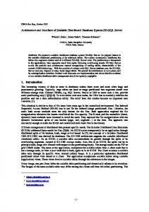
Figure 1: Traffic generated by a node using different associative arrays. Mechanism PAA-scalable PAA-Bloom Bloomier

Re-located objects 26600 26600 26600

Local space (KB) 150.8 31.84 575.3

Table 3: Re-located objects and size of different PAA implementations

6.1

0

Probabilistic Associative Array

In this section we study tradeoffs in the space efficiency and accuracy involved in the configuration and implementation of the PAA. For these results, we have configured the benchmark with 100% locality. In order to use the PAA with TPC-C, we modified the TPC-C keys in order to implement the Feature Extractor Interface according to the static attributes of the objects they represent. Bloom Filter Figure 1 presents the network bandwidth of different implementations of the PAA, compared with another form of probabilistic associative arrays, the Bloomier Filters (B LOOMIER) [5] as the rounds advance in the system. One implementation of the PAA uses regular Bloom filters (PAA-B LOOM) [3], while the other uses a scalable Bloom filter (PAA- SCALABLE) [1]. Both PAAs were configured with α = β = 0.01, and the Bloomier filter’s false positive probability was also set to 0.01. We note that the best solution is the one that allows to propagate in the network only differential updates with regard to the previous state, i.e, the PAA-scalable. Table 3 shows the correspondent local storage requirements at the end of the experiment. As it can be seen, PAA- SCALABLE has higher storage requirements than PAA-B LOOM. This is unsurprising, as scalable bloom filters are known to achieve lower compression than traditional bloom filters when fed with the same data set and configured to yield the same false positive rates [1].

500

% Error Size 0

5 10 15 20 25 Number of relocated data items (Thousands)

30

400

Figure 2: Error probability and rule set size for VFDT However, the storage requirements of both solutions are still considerably smaller than those of Bloomier filters. Machine Learner Figure 2 presents the error probability and space required by the DT to encode the objects moved in every round of the experiment. As more objects are moved in the system, the number of rules increases, leading to an increase in the size taken by this portion of the PAA. However, the machine learner can represent the mapping of 26600 keys in 1000 Bytes, which correspond to 213 rules. Furthermore, it can also be observed that while a significant number of keys is added to the machine learner (around 1000 per round), the error remains relatively stable.

6.2

Leveraging from Locality

This section shows how AUTO P LACER is able to leverage form locality patterns in the workload. The results were obtained with TPC-C, adapted as explained before and with a replication of degree d = 2. Figure 3(a) shows the throughput of AUTO P LACER, compared with the non-optimized system using consistent hashing for different degrees of locality in the workload. In the baseline system, no matter how much locality exists in the workload, since consistent hashing is used to place the items, on average the number of remote accesses does not change. Thus, for all workloads the baseline system exhibits a similar (sub-optimal) behaviour. In the system running AUTO P LACER, locality is leveraged by relocating data items. As times passes, and more rounds of optimization take place, the system throughput increases up to a point where no further optimization is performed. It is interesting to note that, in case there is no locality, the throughput is not affected by the background optimization process. On the other hand, when locality exists, the throughput of the system optimized with AUTO P LACER is much higher than that of the baseline: it can be up to 6 times better for a workload

1000

100% locality 90% locality 50% locality 0% locality baseline

100

10

100% Locality

5

10

15 Time (minutes)

20

25

0.9

0.7 0.6 0.5 0.4 0.3 0.2 0.1 0

5

10

15 Time (minutes)

20

25

0% Locality

Figure 4: Throughput of AUTO P LACER, a directorybased and a consistent hashing-based solution, after a complete optimization process.

100% locality 90% locality 50% locality 0% locality baseline

0.8

90% Locality

30

1 Percentage of remote operations (%)

100

10

0

(a) Throughput with varying degrees of locality.

0

AutoPlacer Directory Baseline

Transaction per second (tx/s)

Transactions per second (TX/s)

1000

30

(b) % of remote operations.

Figure 3: AUTO P LACER performance

with 90% locality, and up to 30 times better in the ideal case of 100% locality. Figure 3(b) helps to understand the improvement in performance by looking at the number of remote invocations that are performed in the system as time evolves. Since the initial setup relies on consistent hashing, both in the baseline and in the optimized system, the average 1 probability of an operation being local is 40 = 2.5% for all workloads. Thus, when the system starts most operations are remote. However, the plots clearly show that the number of remote operations decreases in time when using AUTO P LACER. The plots also show another interesting aspect: although the number of remote operations decreases sharply after a few rounds of optimization, the overall throughput takes longer to improve. This is due to the fact that read transactions access a large number of objects, thus multiple rounds of optimization are required to alleviate the network, which is the bottleneck in these settings. This clearly highlights the relevance of the continuous optimization process implemented by AUTO P LACER. At the end of the experiment, the percentage of operations performed locally is already close to the percentage of locality in the workload; this shows that when the system stabilizes, AUTO P LACER was able to move practically all keys subject to locality. Finally, Figure 4 compares the performance of AUTO -

P LACER and of a directory service-based system. These results were obtained by storing the data relocation map obtained at the end of the entire optimization process into a dedicated directory service. In this case, whenever a node requests a data item that is not stored locally, it contacts the directory service to determine its location, instead of querying the local PAA. The results clearly show that the additional latency for contacting the directory service can hinder perform significantly, independently of the locality of the workload. The plots highlight that, unlike for AUTO P LACER, the performance of directorybased systems can be worse than that achievable by using random placement. This is explainable considering that, with low locality, a large fraction of data accesses is remote, and that directory-based services impose a 2-hop latency, unlike consistent hashing and AUTO P LACER. The speed-ups of AUTO P LACER vs the directorybased solution are significant, i.e. around 2x, even for the high locality scenarios. In these scenarios, the reduction of the number of remote operations leads to less lookups on the directory. However, the cost of accessing a remote data item is, in our testbed, about 2 orders of magnitude larger than that of accessing a local item. As a consequence, also in these scenarios, the cost of remote data accesses dominate the execution time of the requests. Hence, such requests, which suffer from one additional communication hop latency in a directory-based solution, effectively limit the throughput of such a solution leading to considerably worse results than AUTO P LACER.

7

Related Work

A common approach to implementing data placement mechanisms in large scale systems is to manage the data through coarse grain by partitioning it into buckets (also named directories [8] or tablets [6]). Through such partitioning, systems can deploy a centralized com-

ponent which manages the location of all buckets in the system, moving them as required to balance the load on hotspot nodes. While coarse partitioning allows for somewhat manageable directories (maintaining the mapping between objects and nodes), on the other hand, it can reduce the effectiveness of the load balancing mechanisms. Furthermore, to improve data locality, these systems make use of sorted keys: the programmer is responsible for assigning similar keys to related data in order for it to be placed in the same server (or in the same group of servers) [8, 6, 18]. AUTO P LACER does not require the programmer to manually bucketize items. While we benefit from information enabled in the key structure, this information is not used for object placement, it is only used for optimizing the PAA. Also our system can establish a fine grain placement for the most accessed items. As hinted several times in the paper, there is extensive work on defining optimal data placement strategies in multiple contexts. Many of these systems, such as Ursa [30] or Schism [9], attempt to perform optimization at a finer grain than buckets, but require the use of centralized components to compute the placement and to keep the resulting directories with the relocation map. As a result, they suffer from scalability limitations as the number of data items grows. Several works have also attempted to derive distributed versions of the placement algorithm, to avoid the bottleneck of a single centralized component. The work by Leff et al proposes several distributed algorithms to approach the replica placement problem [20], and improvements to this work have been recently proposed in [19] and [31]. These results are not applicable to our system, as they only consider the placement of read-only replicas and not of the object ownership. Furthermore, this solution attempts to relocate all the data in the system, which may lead to scalability limitations similar to those of Ursa or Schism. The work by Vilac¸a et al. [29] presents a Space-Filling Curves-based approach to placing co-related data in the same nodes by relying on user-defined per-object tags. The resulting system can provide good locality if the application is designed to perform actions using the tags, since nodes can locally determine who are the owners of the objects with specific tags. However, unlike our system, this placement is static and encoded by the programmer, and has no relation with the actual data access patterns that may emerge at runtime.

8

Conclusions and Future Work

This paper presented AUTO P LACER, a system aimed at self-tuning data placement in a distributed key value store. AUTO P LACER operates in rounds, and, in each round, it optimizes the placement of the top-k “hotspots”,

i.e. the objects generating most remote operations, for each node of the system. Despite supporting fine-grain placement of data items, AUTO P LACER guarantees one hop routing latency using a novel probabilistic data structure, the PAA, which minimizes the cost of maintaining and disseminating the data relocation map. AUTO P LACER has been integrated in a popular open source (transactional) key-value store, Infinispan, and experimentally evaluated using a porting of the TPC-C benchmark. The results shown that AUTO P LACER can achieve a throughput up to 6 times better than the original Infinispan implementation based on consistent hashing. In this paper we have described how AUTO P LACER can be employed to optimize data placement in presence of static workloads. A detailed discussion and evaluation on how to extend AUTO P LACER to cope with variable workloads will be the subject of a future paper, but, below, we briefly describe a possible approach to achieve this result. AUTO P LACER can be made to operate in epochs. In each epoch, the system operates exactly as described in this paper. A new epoch is started when the need for recomputing data placement is identified, for instance, whenever an abrupt change of the remote access probability is detected [17] in the current epoch. As described in this paper, a new epoch e starts with an empty local lookup table LookupT e and, therefore, in the first iteration, all objects are considered when identifying hotspots. If objects need to be relocated (with regard to the previous epoch), their new position is stored in LookupT e . In fact, the system described before can be seen as a particular case of the general algorithm, where only two epochs are considered: epoch o (defined by consistent hashing) and epoch 1 (the first workload). Also the lookup function would have to be changed. Instead of consulting just the last lookup table, the lookup function would need to consult all the lookup tables in reverse chronological order. Naturally, this would slow down the lookup function after a long series of epochs. However, this could be easily mitigated by a background procedure that would merge the last lookup tables in a new consolidated table (in a process analogous to the one used in several log based file systems).

Acknowledgements The authors wish to thank Zhongmiao Li for his valuable help with validating the initial prototypes of this work. This work was partially supported by Fundac¸a˜ o para a Ciˆencia e Tecnologia (FCT) via the INESC-ID multi-annual funding through the PIDDAC Program fund grant, under projects PEst-OE/ EEI/ LA0021/ 2011, and CMU-PT/ELE/0030/2009 and by the Cloud-TM project (co-financed by the European Commission through the contract no. 257784).

References [1] A LMEIDA , P., BAQUERO , C., P REGUIC¸ A , N., AND H UTCHI SON , D. Scalable bloom filters. Inf. Process. Lett. (Mar. 2007). [2] A MZA , C., C OX , A., AND Z WAENEPOEL , W. Conflict-aware scheduling for dynamic content applications. In Proc. of the 4th USITS (Seattle (WA), USA, 2003). [3] B LOOM , B. Space/ time trade-offs in hash coding with allowable errors. Comm. of the ACM (1970). [4] C HANG , F., ET AL . Bigtable: a distributed storage system for structured data. In Proc. of the 7th OSDI (Seattle, USA, 2006). [5] C HAZELLE , B., K ILIAN , J., RUBINFELD , R., AND TAL , A. The bloomier filter: an efficient data structure for static support lookup tables. In Proc. of the 15th SODA (New Orleans (LA), USA, 2004). [6] C OOPER , B., R AMAKRISHNAN , R., S RIVASTAVA , U., S IL BERSTEIN , A., B OHANNON , P., JACOBSEN , H.-A., P UZ , N., W EAVER , D., AND Y ERNENI , R. Pnuts: Yahoo!’s hosted data serving platform. In Proc. of the 34th VLDB (Auckland, New Zealand, Aug. 2008). [7] C OOPER , B. F., S ILBERSTEIN , A., TAM , E., R AMAKRISHNAN , R., AND S EARS , R. Benchmarking cloud serving systems with ycsb. In Proc. of the 1st SoCC (New York, NY, USA, 2010). [8] C ORBETT, J., ET AL . Spanner: Google’s globally-distributed database. In Proc. of the 10th OSDI (Hollywood, CA, USA, 2012). [9] C URINO , C., J ONES , E., Z HANG , Y., AND M ADDEN , S. Schism: a workload-driven approach to database replication and partitioning. In Proc. of the 36th VLDB (Singapore, Sept. 2010). [10] D E C ANDIA , G., ET AL . Dynamo: amazon’s highly available key-value store. In Proc. of the 21st SOSP (Stevenson, USA, 2007). [11] D OMINGOS , P., AND H ULTEN , G. Mining high-speed data streams. In Proc. of the 6th KDD (Boston, MA, USA, 2000). [12] D OWDY, L., AND F OSTER , D. Comparative models of the file assignment problem. ACM Computing Surveys (1982). [13] F LEISCH , B., AND P OPEK , G. Mirage: a coherent distributed shared memory design. SIGOPS Oper. Syst. Rev. (Nov. 1989). [14] G ARBATOV, S., AND C ACHOPO , J. Data access pattern analysis and prediction for object-oriented applications. INFOCOMP Journal of Computer Science (December 2011). ˜ M ART´I NEZ , M., AND A LONSO , [15] J IM E´ NEZ -P ERIS , R., PATI NO G. Non-intrusive, parallel recovery of replicated data. In Proc. of the 21st IEEE SRDS (Washington, DC, USA, 2002). [16] K RISHNAN , P., R AZ , D., AND S HAVITT, Y. The cache location problem. IEEE/ACM Transactions on Networking (Oct. 2000). [17] L., S., AND L., T. Cusum test for parameter change based on the maximum likelihood estimator. Sequential Analysis: Design Methods and Applications (2004). [18] L AKSHMAN , A., AND M ALIK , P. Cassandra: a decentralized structured storage system. SIGOPS Oper. Syst. Rev. (Apr. 2010). [19] L AOUTARIS , N., T ELELIS , O., Z ISSIMOPOULOS , V., AND S TAVRAKAKIS , I. Distributed selfish replication. IEEE TPDS (Dec. 2006). [20] L EFF , A., W OLF, J., AND Y U , P. Replication algorithms in a remote caching architecture. IEEE TPDS (Nov. 1993). [21] L EUTENEGGER , S., AND D IAS , D. A modeling study of the tpcc benchmark. In Proc. of the SIGMOD Conf. (Washington, D.C., United States, 1993).

[22] M ARCHIONI , F., AND S URTANI , M. Infinispan Data Grid Platform. PACKT Publishing, 2012. [23] M ETWALLY, A., AGRAWAL , D., AND E L A BBADI , A. Efficient computation of frequent and top-k elements in data streams. In Proc. of the 10th ICDT (Edinburgh,Scotland, 2005). [24] M ITCHELL , T. Machine Learning. McGraw-Hill, New York, 1997. [25] P ELUSO , S., ROMANO , P., AND Q UAGLIA , F. Score: A scalable one-copy serializable partial replication protocol. In Proc. of the 13th Middleware (2012), pp. 456–475. [26] P ELUSO , S., RUIVO , P., ROMANO , P., Q UAGLIA , F., AND RO DRIGUES , L. When scalability meets consistency: Genuine multiversion update-serializable partial data replication. In Proc. of the 32nd ICDCS (2012), pp. 455–465. [27] RUIVO , P., C OUCEIRO , M., ROMANO , P., AND RODRIGUES , L. Exploiting total order multicast in weakly consistent transactional caches. In Proc. of the the 17th PRDC (Pasadena, California, USA, Dec. 2011). [28] S TANOI , I., AGRAWAL , D., AND A BBADI , A. E. Using broadcast primitives in replicated databases. In Proc. of the The 18th ICDCS (Washington, DC, USA, 1998). [29] V ILAC¸ A , R., O LIVEIRA , R., AND P EREIRA , J. A correlationaware data placement strategy for key-value stores. In Proc. of the 11th DAIS (Reykjavik, 2011). [30] YOU , G.-W., H WANG , S.-W., AND JAIN , N. Scalable load balancing in cluster storage systems. In Proc. of the 12th Middleware (Lisbon, Portugal, 2011). [31] Z AMAN , S., AND G ROSU , D. A distributed algorithm for the replica placement problem. IEEE TPDS (Sept. 2011).