scalable and efficient outlier detection in large distributed data ... - Fcla

Scalable and Efficient Outlier Detection in Large Distributed Data Sets with Mixed-Type Attributes

by

Anna Koufakou B.S. Athens University of Economics and Business, 1997 M.S. University of Central Florida, 2000

A dissertation submitted in partial fulfillment of the requirements for the degree of Doctor of Philosophy in the School of Electrical Engineering and Computer Science in the College of Engineering at the University of Central Florida Orlando, Florida

Summer Term 2009

Major Professor: Michael Georgiopoulos

c 2009 Anna Koufakou

ii

Abstract

An important problem that appears often when analyzing data involves identifying irregular or abnormal data points called outliers. This problem broadly arises under two scenarios: when outliers are to be removed from the data before analysis, and when useful information or knowledge can be extracted by the outliers themselves. Outlier Detection in the context of the second scenario is a research field that has attracted significant attention in a broad range of useful applications. For example, in credit card transaction data, outliers might indicate potential fraud; in network traffic data, outliers might represent potential intrusion attempts. The basis of deciding if a data point is an outlier is often some measure or notion of dissimilarity between the data point under consideration and the rest. Traditional outlier detection methods assume numerical or ordinal data, and compute pair-wise distances between data points. However, the notion of distance or similarity for categorical data is more difficult to define. Moreover, the size of currently available data sets dictates the need for fast and scalable outlier detection methods, thus precluding distance computations. Additionally, these methods must be applicable to data which might be distributed among different locations. In this work, we propose novel strategies to efficiently deal with large distributed data containing mixed-type attributes. Specifically, we first propose a fast and scal-

iii

able algorithm for categorical data (AVF), and its parallel version based on MapReduce (MR-AVF). We extend AVF and introduce a fast outlier detection algorithm for large distributed data with mixed-type attributes (ODMAD). Finally, we modify ODMAD in order to deal with very high-dimensional categorical data. Experiments with large realworld and synthetic data show that the proposed methods exhibit large performance gains and high scalability compared to the state-of-the-art, while achieving similar accuracy detection rates.

iv

To my parents and to Lela

v

Acknowledgments I would like to take the opportunity to acknowledge a number of individuals for their support during my doctoral work. First, I would like to express many thanks to my adviser, Dr. Georgiopoulos, for providing me with his guidance and support these past many years. I would also like to thank my committee members, Dr. Eaglin, Dr. Kasparis, Dr. Reynolds, and Dr. Turgut for their time and their feedback, as well as Dr. Tace Crouse for her encouragement and advice. I am very grateful to the many friends and colleagues who have shared my graduate experience at UCF with me, especially Pradeep, Jimmy, Moataz, Barry, Sasha, Maria. Also, many thanks to everyone at the UCF Women in EECS group, who have truly encouraged and inspired me this last year. I would also like to acknowledge all my friends outside UCF, especially Ioanna, Andreas, George, Parisa, and Mike. Finally, I would like to thank my parents for their endless encouragement and belief in me, my aunt Lela for her unconditional love, my sister and her family for their support, my aunt Korina for inspiring me, and my extended family for their encouragement. This dissertation acknowledges the support by the National Science Foundation grants: 0341601, 0647018, 0717674, 0717680, 0647120, 0525429, 0806931, 0837332.

vi

TABLE OF CONTENTS

LIST OF FIGURES . . . . . . . . . . . . . . . . . . . . . . . . . . . . . . . . .

xi

LIST OF TABLES . . . . . . . . . . . . . . . . . . . . . . . . . . . . . . . . . . xiv

CHAPTER 1: INTRODUCTION . . . . . . . . . . . . . . . . . . . . . . . .

1

CHAPTER 2: PREVIOUS WORK . . . . . . . . . . . . . . . . . . . . . . .

9

2.1

2.2

Outlier Detection . . . . . . . . . . . . . . . . . . . . . . . . . . . . . . .

9

2.1.1

Statistical/Model-based Approaches . . . . . . . . . . . . . . . . .

9

2.1.2

Distance-based and Clustering Approaches . . . . . . . . . . . . .

10

2.1.3

Density-based Approaches . . . . . . . . . . . . . . . . . . . . . .

12

2.1.4

Other Approaches . . . . . . . . . . . . . . . . . . . . . . . . . . .

13

2.1.5

Approaches for Data Sets with Categorical or Mixed-Type Attributes . . . . . . . . . . . . . . . . . . . . . . . . . . . . . . . .

14

Frequent Itemset Mining (FIM) . . . . . . . . . . . . . . . . . . . . . . .

15

2.2.1

Association Rule Mining and Traditional FIM . . . . . . . . . . .

15

2.2.2

Condensed Representations of FIs (CFIs) . . . . . . . . . . . . . .

18

2.2.3

Other methods . . . . . . . . . . . . . . . . . . . . . . . . . . . .

20

vii

CHAPTER 3: OUTLIER DETECTION FOR CATEGORICAL DATA: ATTRIBUTE VALUE FREQUENCY (AVF) . . . . . . . . . . . . . . . . .

21

3.1

Introduction . . . . . . . . . . . . . . . . . . . . . . . . . . . . . . . . . .

21

3.2

Greedy Algorithm . . . . . . . . . . . . . . . . . . . . . . . . . . . . . . .

22

3.3

FindFPOF . . . . . . . . . . . . . . . . . . . . . . . . . . . . . . . . . . .

24

3.4

Otey’s Method for Categorical Data . . . . . . . . . . . . . . . . . . . . .

25

3.5

Attribute Value Frequency (AVF) . . . . . . . . . . . . . . . . . . . . . .

27

3.6

Experiments . . . . . . . . . . . . . . . . . . . . . . . . . . . . . . . . . .

29

3.6.1

Experimental Setup . . . . . . . . . . . . . . . . . . . . . . . . . .

29

3.6.2

Results and Discussion . . . . . . . . . . . . . . . . . . . . . . . .

30

Summary . . . . . . . . . . . . . . . . . . . . . . . . . . . . . . . . . . .

35

3.7

CHAPTER 4: PARALLEL OUTLIER DETECTION FOR CATEGORICAL DATASETS USING MAPREDUCE: MR-AVF . . . . . . . . . . . .

37

4.1

Introduction . . . . . . . . . . . . . . . . . . . . . . . . . . . . . . . . . .

37

4.2

Background on MapReduce . . . . . . . . . . . . . . . . . . . . . . . . .

38

4.3

MR-AVF . . . . . . . . . . . . . . . . . . . . . . . . . . . . . . . . . . . .

42

4.4

MR-AVF Experiments . . . . . . . . . . . . . . . . . . . . . . . . . . . .

44

4.4.1

Experimental Setup . . . . . . . . . . . . . . . . . . . . . . . . . .

44

4.4.2

Results . . . . . . . . . . . . . . . . . . . . . . . . . . . . . . . . .

45

Summary . . . . . . . . . . . . . . . . . . . . . . . . . . . . . . . . . . .

46

4.5

viii

CHAPTER 5: OUTLIER DETECTION FOR LARGE DISTRIBUTED MIXED-ATTRIBUTE DATA: ODMAD . . . . . . . . . . . . . . . . . . . .

48

5.1

Introduction . . . . . . . . . . . . . . . . . . . . . . . . . . . . . . . . . .

48

5.2

Related Work . . . . . . . . . . . . . . . . . . . . . . . . . . . . . . . . .

50

5.3

Algorithms . . . . . . . . . . . . . . . . . . . . . . . . . . . . . . . . . . .

52

5.3.1

Centralized Algorithm . . . . . . . . . . . . . . . . . . . . . . . .

53

5.3.2

Distributed Algorithm . . . . . . . . . . . . . . . . . . . . . . . .

71

Experiments and Results . . . . . . . . . . . . . . . . . . . . . . . . . . .

74

5.4.1

Experimental Setup . . . . . . . . . . . . . . . . . . . . . . . . . .

74

5.4.2

Results . . . . . . . . . . . . . . . . . . . . . . . . . . . . . . . . .

76

5.4.3

Distributed Experiments . . . . . . . . . . . . . . . . . . . . . . .

80

5.4.4

Additional Experiments . . . . . . . . . . . . . . . . . . . . . . .

81

5.4.5

Discussion . . . . . . . . . . . . . . . . . . . . . . . . . . . . . . .

87

Summary . . . . . . . . . . . . . . . . . . . . . . . . . . . . . . . . . . .

89

5.4

5.5

CHAPTER 6: OUTLIER DETECTION FOR LARGE CATEGORICAL DATA SETS USING NON-DERIVABLE (NDI) AND NON-ALMOST DERIVABLE (NADI) ITEMSETS . . . . . . . . . . . . . . . . . . . . . . .

91

6.1

Introduction . . . . . . . . . . . . . . . . . . . . . . . . . . . . . . . . . .

91

6.2

Algorithms . . . . . . . . . . . . . . . . . . . . . . . . . . . . . . . . . . .

94

6.2.1

95

Outlier Detection based on Frequent Itemsets . . . . . . . . . . .

ix

6.3

6.4

6.2.2

Outlier Detection based on NDIs: FNDI-OD . . . . . . . . . . . . 101

6.2.3

Outlier Detection based on Approximation of NDIs . . . . . . . . 111

Experiments . . . . . . . . . . . . . . . . . . . . . . . . . . . . . . . . . . 113 6.3.1

Experimental Setup . . . . . . . . . . . . . . . . . . . . . . . . . . 113

6.3.2

Results . . . . . . . . . . . . . . . . . . . . . . . . . . . . . . . . . 115

6.3.3

Discussion . . . . . . . . . . . . . . . . . . . . . . . . . . . . . . . 121

Summary . . . . . . . . . . . . . . . . . . . . . . . . . . . . . . . . . . . 127

CHAPTER 7: CONCLUSION . . . . . . . . . . . . . . . . . . . . . . . . . . 129 7.1

Conclusions . . . . . . . . . . . . . . . . . . . . . . . . . . . . . . . . . . 129

7.2

Discussion and Future Work . . . . . . . . . . . . . . . . . . . . . . . . . 131

APPENDIX A: NOTATION . . . . . . . . . . . . . . . . . . . . . . . . . . . 134

APPENDIX B: DATASETS . . . . . . . . . . . . . . . . . . . . . . . . . . . . 136

APPENDIX C: COMPUTATIONAL SAVINGS DUE TO ODMAD CATEGORICAL SCORE . . . . . . . . . . . . . . . . . . . . . . . . . . . . . . . . 142

LIST OF REFERENCES . . . . . . . . . . . . . . . . . . . . . . . . . . . . . 146

x

LIST OF FIGURES

1

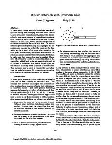
Two-Dimensional example of normal points (shaded regions A and B) and outliers (O1,2 ). . . . . . . . . . . . . . . . . . . . . . . . . . . . . . . . . .

2

2

Example of Frequent Sets, Infrequent Sets, and Sets on Negative Border .

16

3

Greedy Algorithm Pseudocode . . . . . . . . . . . . . . . . . . . . . . . .

23

4

FindFPOF Pseudocode . . . . . . . . . . . . . . . . . . . . . . . . . . . .

25

5

Otey’s Pseudocode (Categorical Data) . . . . . . . . . . . . . . . . . . .

26

6

Example of normal and outlier points from UCI Breast Cancer Dataset. Outlier points are denoted by asterisk. . . . . . . . . . . . . . . . . . . .

28

7

AVF Pseudocode . . . . . . . . . . . . . . . . . . . . . . . . . . . . . . .

29

8

AVF, Greedy, FPOF, and Otey’s runtime performance for simulated data as n, k, and m increase (milliseconds). . . . . . . . . . . . . . . . . . . .

9

33

The flow of data in a MapReduce/GFS architecture for file storage and MapReduce operations (dashed lines indicate control messages, and solid lines indicate data transfer). . . . . . . . . . . . . . . . . . . . . . . . . .

41

10

A pictorial illustration of the WordCount example. . . . . . . . . . . . .

42

11

MR-AVF Pseudocode . . . . . . . . . . . . . . . . . . . . . . . . . . . . .

43

xi

12

Speedup of Parallel AVF algorithm (MR-AVF) as the number of servers in the cluster increases from 1 node to 16 nodes. . . . . . . . . . . . . . .

13

Masking Effect: Outlier point O2 is more irregular than the normal points and outlier point O1 , therefore O2 will likely mask O1 . . . . . . . . . . . .

14

46

54

Scenarios for outlier points and normal points in the continuous space (dots denote normal points, diamonds denote outliers). Outlier points O2 have a high categorical score, while outlier O1 has a low categorical score. In the continuous space, outliers O2 are (a) highly irregular, (b) moderately irregular, or (c) normal, with respect to the rest of the points (normal points and outlier O1 ). . . . . . . . . . . . . . . . . . . . . . . . . . . . .

66

15

First Phase of ODMAD Pseudocode

. . . . . . . . . . . . . . . . . . . .

68

16

Second Phase of ODMAD Pseudocode . . . . . . . . . . . . . . . . . . .

69

17

Categorical value b co-occurs in our dataset with highly infrequent categorical (a) value a only; (b) values a and c. . . . . . . . . . . . . . . . . .

18

74

Speedup of ODMAD as the number of nodes increases from 2 to 16 for the Entire KDDCup 1999 Dataset and Artificial Dataset (1 million normal points and 10 thousand outliers) . . . . . . . . . . . . . . . . . . . . . . .

19

81

Effect to detection rates for ODMAD on the KDDCup 1999 10% dataset varying the lower threshold low sup (upper sup = σ = 10%; ∆scorec = 9, ∆scoreq = 1.6). . . . . . . . . . . . . . . . . . . . . . . . . . . . . . . . .

xii

83

20

Effect to detection rates for ODMAD on the KDDCup 1999 10% dataset varying the upper threshold upper sup (low sup = 2%; σ = 10%; ∆scorec = 9, ∆scoreq = 1.6). . . . . . . . . . . . . . . . . . . . . . . . . . . . . . . .

21

84

Execution Time in seconds as the number of categorical and continuous attributes increases (Entire KDDCup 1999 set). . . . . . . . . . . . . . .

86

22

FI-OD Pseudocode . . . . . . . . . . . . . . . . . . . . . . . . . . . . . .

98

23

NBFI-OD Pseudocode . . . . . . . . . . . . . . . . . . . . . . . . . . . .

99

24

FNDI-OD Pseudocode . . . . . . . . . . . . . . . . . . . . . . . . . . . . 109

25

NBNDI-OD Pseudocode . . . . . . . . . . . . . . . . . . . . . . . . . . . 111

26

Runtime performance for FNDI-OD vs. FI-OD for the Mushroom and KDD1999 sets as σ decreases (MAXLEN = 4). . . . . . . . . . . . . . . 119

27

Effect of MAXLEN on the Correct Detection rates for NBNDI-OD versus NBFI-OD for the Mushroom set and two σ values. . . . . . . . . . . . . . 122

28

Correct Detection for FNADI-OD versus FNDI-OD for the Mushroom set and various δ values. . . . . . . . . . . . . . . . . . . . . . . . . . . . . . 125

xiii

LIST OF TABLES

1

Algorithms presented in this dissertation and their characteristics w.r.t. attribute type, time complexity for categorical (mc ) and continuous (mq ) attributes, location of the dataset, and challenges they address.

. . . . .

8

2

AVF, Greedy, FPOF, and Otey’s Accuracy Results on Real Datasets . .

32

3

Runtime of AVF, Greedy, FPOF, and Otey’s Approaches in seconds for the simulated data with varying number of data points, n. . . . . . . . .

4

Detection Rate of ODMAD vs. Otey’s on KDDCup 1999 (10%, Entire Training and Test Sets.) . . . . . . . . . . . . . . . . . . . . . . . . . . .

5

79

Execution Time (seconds) for ODMAD versus Otey’s on the KDDCup 1999 Datasets. . . . . . . . . . . . . . . . . . . . . . . . . . . . . . . . . .

6

34

80

ODMAD Detection Rate using only categorical attributes: all infrequent subsets versus only pruned candidates, using the KDDCup 1999 10% Train Dataset. . . . . . . . . . . . . . . . . . . . . . . . . . . . . . . . . . . . .

7

88

Dataset Details: Number of rows, columns, single distinct items, percentage of outliers in the dataset. . . . . . . . . . . . . . . . . . . . . . . . . 114

xiv

8

Comparison of Correct Detection (False Alarm) rates of FNDI-OD, FIOD, NBNDI-OD, and NBFI-OD for BC as k varies (σ = 10%; actual outliers: 39). . . . . . . . . . . . . . . . . . . . . . . . . . . . . . . . . . . 116

9

Comparison of Correct Detection (False Alarm) rates of FNDI-OD, FI-OD, NBNDI-OD, and NBFI-OD for (a)Mushroom and (b)KDD1999 Datasets. 116

10

Generated sets and Runtime performance for NDI- versus FI-based methods on the Mushroom and the KDD1999 set. Time is shown in seconds as Time for Phase 1 (Set Mining)/Time for Phase 2 (Outlier Scoring). . . 118

11

Comparison of Correct Detection (False Alarm) rates, Generated Sets, and Runtime Performance in seconds for FI-OD, FNDI-OD, and FNADI-OD for (a)Mushroom and (b)KDD1999 Data Sets. . . . . . . . . . . . . . . . 123

12

Frequency of distinct values (items) in Mushroom and KDD1999 Data Sets. . . . . . . . . . . . . . . . . . . . . . . . . . . . . . . . . . . . . . . 127

13

Notation used in this dissertation. . . . . . . . . . . . . . . . . . . . . . . 135

14

Datasets: Number of rows, columns, and percentage of outliers. . . . . . 137

xv

CHAPTER 1 INTRODUCTION

The need for data mining, i.e. extracting knowledge from the data in the form of useful and interesting models and trends, is of greater importance today than ever before, due to the massive amount of data existing in databases all over the world. For example, it was projected that, by the end of 2007, the Sloan Digital Sky Survey1 will have produced over 40 terabytes of image data, and over 3 terabytes of processed data. Mining for outliers in data is an important data mining research field with many applications such as network intrusion detection [DEK02]. Outlier detection approaches focus on discovering patterns that occur infrequently in the data, as opposed to many traditional data mining techniques, such as association rule mining or frequent itemset mining, that attempt to find patterns that occur frequently in the data. One of the most widely accepted definitions of an outlier pattern is provided by Hawkins [Haw80]:

“An outlier is an observation that deviates so much from other observations as to arouse suspicion that it was generated by a different mechanism”.

Outliers are frequently treated as noise that needs to be removed from a dataset in order for a specific model or algorithm to succeed (e.g. points not belonging in clusters in a clustering algorithm). Alternatively, outlier detection techniques can lead to the 1

http://www.sdss.org

1

y

O1 A

B O2

x Figure 1: Two-Dimensional example of normal points (shaded regions A and B) and outliers (O1,2 ). discovery of important information in the data (“one person’s noise is another persons signal” [KN98]). Finally, outlier detection strategies can also be used for data cleaning as a step before any traditional mining algorithm is applied to the data. It should be noted that this dissertation deals with unsupervised outlier detection, i.e. our methods do not assume labeled training data. Also, our techniques make the implicit assumption that the percentage of normal points is far larger compared to the percentage of outliers in the data set. A pictorial two-dimensional example is shown in Figure 1. This Figure contains two groups or clusters of normal data points, denoted by shaded regions A and B, a single outlier point, O1 , and a group of outlier points, O2 . Examples of applications where the discovery of outliers is useful include: detecting irregular credit card transactions which may indicate potential credit card fraud [BH02]; identifying patients who exhibit abnormal symptoms due to their suffering from a specific

2

disease or ailment [PJ01]; detecting irregularities and potential fraud in accounting data [BKA06], among others. Many existing approaches are based on assumptions of a normal model/distribution or on calculating distances between each and every data point. For example, if we assume that outliers are those points that are most distant from the rest of the points, in Figure 1, outlier O1 is easily flagged as an outlier as being far from the rest of the points. However, outlier points in region O2 are very close to normal points in region A and thus might be more difficult to be detected as outliers. Therefore, more sophisticated algorithms are needed that can address these and other issues, described below. In general, the performance and even the applicability of the majority of existing methods are limited by the characteristics of datasets currently available. Specifically, important challenges faced by outlier detection methods and addressed in this dissertation include the following:

(a) datasets might have large numbers of data points and dimensions, (b) datasets might contain categorical attributes or a mixture of categorical and continuous attributes, (c) challenges caused by the high dimensionality of the data, e.g. datasets might be sparse in the continuous space, or dense in the categorical space, and (d) the points in the dataset might be distributed among different locations.

In the following paragraphs, we briefly describe each of the above four challenges.

3

Large Number of Data Points and Dimensions: The first challenge mentioned earlier is related to the large size of today’s data. With the explosion of technology, the size of data for a particular application has grown and will continue to grow; terabytescale data is now common, e.g., Wal-Mart had 460 terabytes of data in 2004 [Hay04]. Hence, successful outlier detection strategies must scale well as the number of data points and dataset dimensionality grow. The size of the datasets today also leads to the need for large, parallel machines and associated parallelizable outlier detection algorithms, which must also be easily balanced over a number of cluster nodes. Types of Attributes: A second issue is that the majority of existing research in outlier detection has focused on data sets with a specific attribute type, i.e. only numerical attributes or ordinal attributes that can be directly mapped into numerical values, while there is some research using only categorical attributes. Quite often, when we have data containing categorical attributes, for example, it is assumed that the categorical attributes could be easily mapped into numerical values. However, there are cases, where mapping categorical attributes to numerical attributes is not a straightforward process, and the results greatly depend on the mapping that is used, e.g., the mapping of a marital status attribute value (married or single) or a person’s profession (engineer, financial analyst, etc.) to a numerical value. In the case of continuous attributes, algorithms designed for categorical data often use discretization techniques to map intervals of continuous space into discrete values. Among unsupervised methods, i.e. those that do not use class information, popular algorithms include equal-width or equal-frequency binning. These methods might not produce good

4

results when the distributions of the continuous attribute values are not uniform, and the resulting discretized ranges are significantly affected by outliers [Cat91]. In our case, for example, values that are associated with normal points and values associated with outliers might be combined in the same bin, which makes the outlier detection task more difficult. High Dimensionality of the Data: A third issue is due to the large number of dimensions in the dataset. In the continuous space, due to the large dimensionality, the dataset becomes sparse. In this type of setting, traditional concepts such as Euclidean distance between points, and nearest neighbor, become irrelevant [ESK03]. Employing dissimilarity measures that can handle sparse data becomes imperative. In addition, inspecting several, smaller views of the large, high-dimensional data can help uncover outliers, which would otherwise be masked by other outlier points if one were to look at the entire dataset at once. In the categorical space, certain datasets may contain many strong correlations, and are typically characterized by categorical values with high frequency and many frequent patterns [ZH05]. As a result, there might be a large number of combinations of these values to generate and store. In general, outlier detection in large high-dimensional data with many categorical values will also face issues if they are based on Frequent Itemsets [AS94]. Distributed Datasets: A fourth issue is that data may be distributed among different sites belonging to the same or different organizations. Moreover, each of these sites might contain large amounts of data. This is an issue that has to be taken into account

5

for any data mining algorithm developed on such a platform, as for example moving or copying large amounts of data from site to site or storing all the data in one site in order to mine the dataset as a whole would be prohibitive. Besides the cost and performance issues, there are also very important issues related to data ownership and control which prohibit organizations from sharing data. Therefore, in order to deal with the distributed nature of the data, the outlier detection algorithms must minimize communication overhead and synchronization overhead between the different sites in which the data reside, as well as the scans over the data. The aim of this dissertation is to propose novel outlier detection techniques that are scalable and exhibit acceptable runtime performance given data sets that might be large, high-dimensional, geographically distributed, and contain categorical or a mixture of categorical and continuous attributes. In this dissertation, we propose algorithms to address the challenges outlined above due to current data sets. Specifically, our contributions are as follows:

• We propose a fast and scalable outlier detection method for categorical data, called Attribute Value Frequency (AVF). AVF, presented in Chapter 3, uses the frequency of each attribute value to compute an anomaly score for each data point. AVF is experimentally shown to be significantly faster than the previous techniques, while maintaining comparable detection accuracy. • We propose a parallel version of AVF using the MapReduce [DG04] paradigm of parallel programming, called MR-AVF (Chapter 4). MR-AVF is simple and easy

6

to implement, and using MapReduce ensures that MR-AVF is fault tolerant and has load balancing. • We propose a method for large high-dimensional data that contain both categorical and continuous attributes, called Outlier Detection for Mixed Attribute Data (ODMAD) (Chapter 5). ODMAD uses Frequent Itemset Mining (FIM) [AS94] to compute anomaly score for the categorical space, and a cosine distance for the continuous space. ODMAD is fast, scales linearly with the number of data points, and uses two data passes. Furthermore, ODMAD can deal with sparse continuous data, exhibits an overall higher detection rate, a lower false positive rate, and runs orders of magnitude faster than the state-of-the-art outlier detection strategies. • We extend ODMAD for datasets that are distributed among different geographical sites (Chapter 5). The distributed version of ODMAD consists of two phases with low communication and synchronization overhead, and exhibits close to linear speedup. • We present outlier detection methods that employ a condensed representation of frequent itemsets, Non-Derivable Itemsets (NDIs) [CG02], to efficiently deal with high-dimensional dense categorical data (Chapter 6). These NDI-based methods exhibit much better scalability and runtime performance and similar detection accuracy rates compared to their FIM-based counterparts for the datasets we experimented with.

7

Table 1: Algorithms presented in this dissertation and their characteristics w.r.t. attribute type, time complexity for categorical (mc ) and continuous (mq ) attributes, location of the dataset, and challenges they address. Algorithm Attribute Time Complexity Data Addresses Type mc mq Location Challenges AVF categorical linear local (a), (b) MR-AVF categorical linear cluster (a), (b), (d) ODMAD mixed exponential linear local (a), (b), (c) D-ODMAD mixed exponential linear distributed (a) - (d) NDI-based OD categorical exponential local (a), (b), (c) Table 1 includes a list of the algorithms proposed in this dissertation and their characteristics as illustrated in the previous paragraphs. The organization of this dissertation is as follows. The next chapter (Chapter 2) provides a thorough literature review of Outlier Detection algorithms. It also includes a review of Frequent Itemset Mining (FIM) and Condensed Representations of Frequent Itemsets (CFI). Chapters 3 through 6 describe the different contributions proposed in this dissertation. Finally, Chapter 7 provides a summary of our work as well as directions for future research.

8

CHAPTER 2 PREVIOUS WORK

In this chapter we provide an overview of the previous work in Outlier Detection, as well as a review of the work in Frequent Itemset Mining and Condensed Frequent Itemset Representations.

2.1

Outlier Detection

The existing outlier detection work can be categorized as follows: Statistical/Modelbased, Distance-based and Clustering, Density-based, other approaches, and approaches for categorical and mixed-type attribute data.

2.1.1

Statistical/Model-based Approaches

Statistical outlier detection was one of the earliest approaches dating back to the 19th century [Edg87]. Statistical-based methods assume that a parametric model, which is usually univariate, describes the distribution of the data [BL78]. Multivariate statistical approaches have been proposed, including use of robust (or less affected by outliers) estimates of the multidimensional distribution parameters, e.g. minimum covariance

9

determinant (MCD) and minimum volume ellipsoid (MVE) [Rou85, RLW87]. One inherent problem of statistical-based methods is finding the suitable model for each dataset and application. Also, as data increases in dimensionality, it becomes increasingly more challenging to estimate the multidimensional distribution [AY01, TSK05]. As the data increases in dimensionality, data is spread through a larger volume and becomes sparse. In addition to the slowing effect this has on performance, it also spreads the convex hull, thus distorting the data distribution (“Curse of Dimensionality” [HA04]). This can be alleviated by preselecting the most significant features to work with (e.g. [AB94]), projecting to a lower-dimensional subspace [AY01]), or applying Principal Component Analysis (PCA). Another approach to deal with higher dimensionalities is to organize data points in convex hull layers according to their peeling depth, based on the idea that outliers are data objects with a shallow depth value, e.g. [PS85]. In practice, however, the complexity lower bound is Ω(nm/2 ) for n data points and m dimensions and perform acceptably only for m ≤ 2.

2.1.2

Distance-based and Clustering Approaches

Distance-based techniques do not make assumptions for the data since they basically compute the distance between each point. For example, Knorr et al. in [KN98] proposed a k-NN approach where, if m of the k nearest neighbors of a point are within a specific distance d, then the point can be classified as normal. Knorr et al. in [KNT00] define a point as an outlier if at least p% of the points in the dataset lie further than distance

10

d from it. These methods exhibit high computational complexity (e.g. nearest neighbor based methods have quadratic complexity with respect to the number of data points) which renders them impractical for really large datasets. Several methods may be employed to make the k-NN queries faster (to achieve linear or logarithmic time), such as an indexing structure (e.g. KD-tree, or X-tree); however these structures have been shown to break down as the dimensionality grows [BS03]: for example, Breunig et al. in [BKN00] used an X-tree index and state that its performance degenerated for dimensionality ≥ 10. Bay et al. in [BS03] proposed a distance-based algorithm based on randomizing the data for efficient pruning of the search space, which in practice has complexity close to linear. This method was shown to have lower accuracy and slower performance for large data when compared to the method in [OGP06]. More recently, there have been efforts toward distance-based approaches in sub quadratic time.

Angiulli et al.

in [AP05] used a Hilbert Space Filling Curve to assist with

k-NN computations; however their method requires m+1 scans of the data where m is the dataset dimensionality, which again might be impractical for distributed, highdimensional data. Besides efficiency, a general limitation of distance-based methods is apparent in complex datasets that contain outliers which are only obvious when one looks locally at the neighborhood of each point. Distance-based methods using a global outlier criterion fail to identify these outliers. Several clustering methods can be used (e.g. k-means, k-medoids, etc.) to form clusters, based on the idea that outliers are points not included in formed clusters. Another idea [She02] is using a graph to reflect the connections between each and every

11

point, then to find the difference (distance) between a point and its neighboring points on a connected graph so that the outliers are those with distance greater than a given threshold; however this technique is applicable only in cases when a graph of the data can be constructed. In general, all the clustering-based methods rely on the concept of the clusters to define the outliers and thus they are focused in optimizing clustering, not outlier detection [KNT00].

2.1.3

Density-based Approaches

Density-based methods estimate the density distribution of the input space and then identify outliers as those lying in regions of low density. Older examples include using Gaussian Mixture Models (GMMs) e.g. [RT94]. Breunig et al. in [BKN00] assign a degree of outlier-ness to each data point, the local outlier factor (LOF), based on the local density of the area around the point and the local densities of its neighbors, relying on a user-given minimum number of points. Extensions include Local Correlation Integral (LOCI) which uses statistical values to avoid user-entered parameters [PKG03], and using kernel density functions [LLP07]. These techniques are able to detect outliers that are missed by techniques with a single, global criterion, such as distance-based techniques [KNT00]. These methods are also based on distance computations which might be inappropriate for categorical data, and again not straightforward to implement in a distributed setting.

12

In addition, high-dimensional data is almost always sparse, which creates problems for density-based methods [TSK05]. In such data, the traditional Euclidean notion of density, i.e. number of points per unit volume, becomes meaningless. The increase in dimensionality leads to increase of volume, and density tends to zero as the number of dimensions grows much faster than the number of data points [ESK03]. The notion of a nearest neighbor or a similar data point does not hold as well because the distance between any two data points becomes almost identical [BGR99]. To deal with sparse data, Ertoz et al. in [ESK03] use the cosine function and shared nearest neighbors to cluster data with high dimensionality.

2.1.4

Other Approaches

Other outlier detection efforts include Support Vector methods, e.g., [TD04], and Replicator Neural Networks [HHW02] among others. There has been much work related to intrusion detection, e.g. [LEK03]. Many methods published in this area are particular to intrusion detection and cannot easily be generalized to other outlier detection areas. Finally, a thorough survey on outlier detection can be found in [HA04], and a more recent one in [CBK09]. A review on fraud detection can be found in [KLS04].

13

2.1.5

Approaches for Data Sets with Categorical or Mixed-Type Attributes

Most of the techniques in the previous sections are geared toward numerical data and thus are more appropriate for numerical datasets or ordinal data that can be easily mapped to numerical values. In the case of categorical data, there is little sense in ordering categorical values, then mapping them to numerical values and computing distances, e.g., distance between values such as TCP Protocol and UDP Protocol [OGP06]. Another limitation of previous methods is the lack of scalability with respect to number of points and/or dimensionality of the dataset. Outlier detection techniques for categorical data have recently appeared in the literature. He et al. [HXD06] propose an outlier detection method based on the idea of Entropy [SPS48]. The methods in [HXH05, OGP06] use the concept of Frequent Itemset Mining (FIM) [AS94] in order to assign an outlier score to each data point based on the subsets this point contains. These techniques are presented and contrasted with our proposed method in Chapter 3. Otey et al. in [OGP06] propose a distributed and dynamic outlier detection method for data with both categorical and continuous attributes. This method combines categorical and continuous data as follows: for each set of categorical values (itemset), X, isolate the data points that contain set X, then calculate the covariance matrix of the continuous values of these points. A point is likely to be an outlier if it contains infrequent categorical sets, or if its continuous values differ from the covariance. We present more details on this method in Chapter 5.

14

The aforementioned FI-based methods do well with respect to runtime performance and scalability with the tested datasets. Nevertheless, these outlier detection techniques rely on mining and using frequent sets, and will face problems with speed and memory requirements when applied to dense data or when the σ threshold is set too low. This is a well-known problem for frequent set mining and addressed in Chapter 6. The previous work related to Frequent Itemset Mining and proposed solutions to address this issue are discussed in the next section.

2.2

2.2.1

Frequent Itemset Mining (FIM)

Association Rule Mining and Traditional FIM

Association Rule Mining (ARM) is a very popular data mining technique, which involves the extraction of relationships which exist among the data. Initially intended to tackle market basket analysis, i.e. to explore consumer trends in terms of their purchases [BMU97], ARM has been proven useful in a plethora of other applications, e.g. climate prediction [ZH04]. An association rule is an implication of the form “{diapers, milk} → {baby powder}”, which means that people who buy diapers and milk also tend to buy baby powder. Let I = {i1 , i2 , . . . , ir } be a set of r items in a database D. Each transaction (row) T in D is a set of items such that T ⊆ I. Given X, a set of some items in I, we say that T contains X if X ⊆ T . The support of X, supp(X), is the percentage of transactions in

15

a: 5

ab: 4

Frequent

ac: 3

abc: 3

Infrequent

b: 4

c: 3

ad: 3

bc: 3

abd: 2

acd: 1

d: 3

bd: 2

cd: 1

bcd: 1

abcd: 1

Figure 2: Example of Frequent Sets, Infrequent Sets, and Sets on Negative Border D that contain X. We say that X is frequent if it appears at least σ times in D, where σ is a user-defined threshold. A set X belongs in the negative border of the frequent sets, if all subsets of X are frequent but X itself is infrequent. Figure 2 depicts an example dataset with the resulting frequent sets and negative border sets. For example, set bd is on the negative border, but set abd is not, as it contains a subset bd that is infrequent. Given a minimum threshold σ, mining of association rules contains two distinct phases: (a) find frequent itemsets, i.e. those with frequency no less than σ, and (b) generate the confident, or interesting rules which contain the frequent itemsets. The first problem of finding the frequent itemsets, which is referred to as Frequent Itemset Mining (FIM), has been identified as the most complex of the two. The main idea behind all algorithms for mining frequent (or large) itemsets, can be described as follows: in the first pass over the data, count the support of individual items, and determine which have minimum support (large or frequent). Then, in the next data

16

pass, use only those itemsets that were found to be large or frequent in the previous pass, in order to generate new potentially large itemsets, called candidate itemsets, and count the support for these candidate itemsets. The frequent candidate itemsets, i.e. those that pass the minimum support threshold, are used to construct the candidate itemsets for the next pass, and so on. This loop ends when no new large itemsets can be found. Agrawal and Srikant introduced the first efficient FIM algorithm, called Apriori [AS94]. The difference between the Apriori algorithm and the prior research is in the way it generates the aforementioned candidate itemsets, and also in the way the candidates are counted in each pass. Apriori’s central property is: “If A is a frequent itemset, then every subset of A is a frequent itemset”. What ensues from this statement is that, once a set has been found infrequent, not only can it be pruned, but all the itemsets that contain it can be pruned as well, as they are also infrequent. For example, if set ab has been found to be infrequent, then itemsets abc, abe, abce, etc., that contain set ab, cannot be frequent, so they too can be pruned. There are several algorithms in the literature to improve different aspects of Apriori, e.g.: DIC [BMU97], which dynamically counts candidates of varying length to reduce number of scans; DHP [PCY95], which collects approximate counts to rule out candidates that cannot possibly be frequent; FP-Growth [HPY04], which stores the transactions in an FP-tree, a trie structure where every item contains a list of all the transactions that contain that item. Also there are several ARM implementations online [Bod03, Bor03, Goe05].

17

2.2.2

Condensed Representations of FIs (CFIs)

Apriori-inspired algorithms perform well with sparse data sets, such as market-basket data, where the frequent patterns are short, but they face problems for dense data. Even with candidate pruning in Apriori, the resulting frequent itemsets might still be numerous, an issue exacerbated when these sets contain millions of items or the σ threshold is too low. The problems that FIM algorithms face with such data is not due to design or implementation of the specific FIM algorithm, but the large number of FIs that are generated. To solve this issue much work has been conducted toward Condensed Representations of FIs (CFIs) e.g. [AAP00, ZH05, CG07]. The goal of these methods is to find a much smaller group of representative sets, from which one can deduce all FIs. Many CFIs have been proposed, which we briefly describe next (more details can be found in [CRB04]). A maximal set is a frequent set that is not a subset of any other frequent itemset [AAP00]. A closed set is a set with support such that there is no superset with support equal to it [PBT99]. Let M be the set of maximal sets and C the set of closed sets. Even though in theory M and C can be exponential in the number of items, in practice, C can be orders of magnitude smaller than the number of frequent sets (especially for dense data), while M can be orders of magnitude smaller than C. Closed sets are lossless in the sense that the exact frequency of all FIs can be determined from C, while M leads to a loss of information (since subset frequency is not kept)[ZH05]. Once a given support threshold is known as well as all frequent closed

18

itemsets with their supports, the rest of the frequent itemsets and their supports can be generated. If an itemset I has at least one superset in the set of all frequent closed itemsets (FreqClosed ), then the supp(I) = supp(cl(I)) where cl(I) is the smallest superset of I in FreqClosed. The reader is reminded that the Apriori Principle states that if an itemset is frequent, then all of its subsets are frequent. Thus, the itemset I in this case is frequent. δ-free sets [BBR00] can be used as a δ-adequate representation for FIs. If we know that the association rule abc → d is nearly an exact rule (i.e. it is true for “most” of the dataset), we can approximate the frequency of set abcd using the frequency of abc. A δ-strong rule is an association rule of the form X ⇒δ a, where X ⊆ I, a ∈ I\X, and δ is a natural number. The rule is valid if it is not violated in more than δ transactions. An itemset Y is δ-free if there is no valid δ-strong rule X ⇒δ a such that X ⊂ Y , a ∈ Y , and a ∈ / X. Given any database D, the set of all frequent δ-free sets can be used to approximate the support of the frequent non-δ-free sets [BBR00]. The authors in [CG07] propose determining bounds on the support of an itemset I, based on the supports of subsets of I. An itemset I is called derivable when its support can be exactly deduced from the support of its subsets [CG07]. Derivable itemsets represent redundant information and can be pruned, so that Non-Derivable Itemsets (NDIs) can form a condensed representation. NDIs have been shown to be significantly more concise than the complete FI collection, and in many cases smaller than the previously mentioned representations [CG05].

19

2.2.3

Other methods

Besides condensed representations, other types of patterns have been proposed and used as a step prior to a data mining tasks such as clustering. For example, [XPS06] used highly-correlated association patterns called hyperclique patterns [XTK06] as a cleaning step to filter out noisy objects, resulting in better clustering performance and higher quality associations. The authors in [HXY07] use hyperclique patterns to detect off-topic documents. The authors in [WK06] proposed summary sets in an effort to summarize categorical data for clustering; summary sets were proven to be closed sets. Finally, in [JC08] a support approximation and clustering method was proposed to mine FIs in the dataset.

20

CHAPTER 3 OUTLIER DETECTION FOR CATEGORICAL DATA: ATTRIBUTE VALUE FREQUENCY (AVF)

3.1

Introduction

In this chapter, we introduce an fast outlier detection strategy for categorical data, called Attribute Value Frequency (AVF) [KOG07]. We compare AVF with existing outlier detection methods with respect to runtime performance as well as outlier detection accuracy. These previous efforts have not been contrasted to each other using the same datasets. The first method by He et al. [HXD06] is an outlier detection method based on the idea of Entropy. The second technique by Otey et al. [OGP06] focuses on datasets with mixed attributes (both categorical and numerical). The third technique is by He et al. [HXH05]. Both methods in [HXH05, OGP06] compute an outlier score for each data point using the concept of Frequent Itemsets [AS94]. Wei et al. [WQZ03] also deal with outliers in categorical datasets using frequent itemsets, as well. In fact, they use hyperedges to store frequent itemsets and the data points that contain these frequent itemsets; since their method is similar to that in [HXH05], it was not considered in our experiments. Finally, Yu et al. [YQL06] use mutual reinforcement to discover outliers in a mixed attribute space; however their method focuses on a different outlier detection problem than the one described in this dissertation

21

(“instead of detecting local outliers as noise, [they] identify local outliers in the center, where they are similar to some clusters of objects on one hand, and are unique on the other.” [YQL06]). Experimentation with real and artificial data sets show that AVF has a significant performance advantage, and scales linearly as the data set increases in number of points and number of dimensions. In addition, AVF is efficient for large and geographically distributed data sets as it performs only one dataset scan.

3.2

Greedy Algorithm

The algorithms in [HXD06] are based on the assumption that outliers are likely to be the points that the dataset as a whole has less “uncertainty” or “disorder” if these outliers are removed from the data. In particular, they propose to identify a small subset (of size k) of the data points which contribute the most to the “disorder” of the dataset. The idea of Entropy, or uncertainty, of a random variable is attributed to Shannon [SPS48]. Formally, if X is a random variable, S(X) is the set of values that X can take, and p(x) is the probability function of X, the entropy, E(X), is defined as follows:

E(X) = −

X

p(x) log2 p(x)

(3.1)

x∈S(X)

Given X = {X1 , X2 , . . . , Xm }, a dataset containing m attributes, and the assumption that the attributes of X are independent, the Entropy of X, E(X), is equal to the sum

22

Input : Database D (n points × m attributes), Target number of outliers - k Output: k detected outliers 1 2 3 4 5 6 7 8 9 10 11 12 13 14 15 16

Label all data points as non-outliers; foreach point xi , i = 1 . . . n do foreach attribute l, l = 1 . . . m do Count frequency f (xil ) of attribute value xil ; end end Calculate initial Entropy of dataset, E; while not k scans do foreach normal point xi , i = 1 . . . n do xi ← outlier; ∆i := decrease in entropy E by removing xi ; end if decrease ∆i is max then Add xi to set of k outliers; end end Figure 3: Greedy Algorithm Pseudocode

of the entropies of each one of the m attributes, and is defined as follows:

E(X) = E(X1 ) + E(X2 ) + . . . + E(Xm )

(3.2)

He et al. introduce a Local-Search heuristic-based Algorithm (LSA) in [HDX05], and a Greedy Algorithm in [HXD06] both relying on the entropy idea mentioned above. Since the Greedy algorithm is superior to LSA, we will only discuss the Greedy algorithm. The Greedy algorithm takes as input the desired number of outliers (k). All points in the set are initially designated as non-outliers. At the beginning, the frequencies of all attribute values are computed, as well as the initial entropy of the dataset. Then, Greedy conducts k scans over the data to determine the top k outliers. During each scan, every non-outlier is temporarily removed from the dataset and the total

23

entropy is recalculated. The non-outlier point that results in the maximum decrease for the entropy of the entire dataset is the outlier data-point removed by the algorithm in each scan. Pseudocode for Greedy is provided in Figure 3. The complexity of Greedy is O(k ×n×m×q) , where k is the target number of outlier points, n designates the number of points in the dataset, m is the number of attributes, and q is the number of distinct attribute values, per attribute. If the number of attribute values per attribute, q, is small, the complexity of Greedy becomes O(k × n × m).

3.3

FindFPOF

Frequent Itemset Mining (FIM) was introduced in the Literature Review Section 2.2. He et al. in [HXH05] observe that, since frequent itemsets are “common patterns” that are found in many of the points of the dataset, outliers are likely to be the points that contain very few common patterns or subsets. They define a Frequent Pattern Outlier Factor (FPOF) for every data point, x, based on the support of the frequent itemsets contained in x. In addition, they use a contradictness score to better explain the outliers and not to detect the outliers, so it is omitted from our discussion. The FPOF outlier score is calculated as follows: X F P OF Score(xi ) =

supp(F )

F ⊆xi ∧ F ∈F I

24

|F I|

(3.3)

Input : Database D (n points × m attributes), Target number of outliers - k, minimum support σ Output: k detected outliers 1 2 3 4 5 6 7 8 9

Label all data points as non-outliers; F I = Get all frequent itemsets(D, σ); foreach point xi , i = 1 . . . n do foreach F ⊆ xi ∧ F ∈ F I do F P OF Score(xi ) += supp(F ); end F P OF Score(xi ) /= |F I|; end Return k outliers with mini (F P OF Score); Figure 4: FindFPOF Pseudocode

The above score is the sum of the support of all the frequent subsets F contained in point xi , over the total number of frequent sets in dataset D, |F I|. Data points with lower FPOF scores are likely to be outliers since they contain fewer common subsets. The FPOF algorithm runs a FIM algorithm such as Apriori [AS94] first, to identify all frequent itemsets in dataset D given threshold σ, then calculates the FPOF outlier score for each data point, to identify the top k outliers (see pseudocode in Figure 4).

3.4

Otey’s Method for Categorical Data

The method by Otey et al. in [OGP06] is also based on frequent itemsets. They assign to each point an anomaly score inversely proportional to its infrequent itemsets. They also maintain a covariance matrix for each itemset to handle continuous attributes; we omit this part since our focus is on categorical data.

25

Input : Database D (n points × m attributes), Target number of outliers - k, minimum support σ Output: k detected outliers 1 2 3 4 5 6 7 8

Label all data points as non-outliers; F I = Get all frequent itemsets(D, σ); foreach point xi , i = 1 . . . n do foreach possible I ⊆ xi ∧ I ∈ / F I do OteyScore(xi ) += 1 / |I|; end end Return k outliers with maxi (OteyScore); Figure 5: Otey’s Pseudocode (Categorical Data)

Specifically, they calculate the following score for each data point xi :

OteyScore(xi ) =

X d⊆xi ∧ d∈F / I

1 |d|

(3.4)

which is explained as follows: given subsets d of xi which are infrequent, i.e. support of d is less than σ, the anomaly score of xi will be the sum of the inverse of the length of d. If a point has few frequent itemsets, its outlier factor will be high, so the outliers are the k points with the maximum outlier score in Equation (3.4). This algorithm also first mines the data for FIs, then calculates an outlier score for each point (see pseudocode in Figure 5). The authors state that the execution time is linear to the number of data points, but exponential to the number of categorical attributes.

26

3.5

Attribute Value Frequency (AVF)

The algorithms discussed so far do scale linearly with respect to the number of data points, n. However, Greedy (section 3.2) still needs k scans over the dataset to find k outliers, a disadvantage for the case of very large datasets that are potentially distributed among different sites. On the other hand, the Frequent Itemset Mining (FIM)-based approaches (sections 3.3 and 3.4) need to create a potentially large space of subsets or itemsets, and then search for these sets in each and every data point. These techniques can become extremely slow for low values of the σ threshold, as more and more candidate itemsets need to be examined. In this section we present a simpler and faster approach to detect outliers that minimizes the scans over the data and does not need to create or search through different combinations of attribute values or itemsets. We call this outlier detection algorithm Attribute Value Frequency (AVF) algorithm. It is intuitive that outliers are those points which are infrequent in the dataset. Additionally, an ideal outlier point in a categorical dataset is one whose each and every attribute value is extremely irregular (or infrequent). The infrequent-ness of an attribute value can be measured by computing the number of times this value is assumed by the corresponding attribute in the dataset. Lets assume that the dataset contains n data points, xi , i = 1 . . . n. If each data point has m attributes, we can write xi = [xi1 , . . . , xil , . . . , xim ], where xil is the value of the l-th attribute of xi . Following the reasoning given above, a good indicator or score to

27

Data point 1 2 3 4 5 6 *7 8 9 10 11 * 12

1 1 2 1 4 4 6 7 3 1 3 5 2

2 1 1 1 1 1 1 3 1 1 2 1 5

Attributes 3 4 5 6 1 1 2 10 1 1 2 1 1 1 2 3 1 1 2 1 1 1 2 1 1 1 2 1 2 10 5 10 1 1 2 1 1 1 2 1 1 1 1 1 1 1 2 1 3 3 6 7

7 3 2 3 2 3 3 5 2 3 2 2 7

8 1 1 1 1 1 1 4 1 1 1 1 5

9 1 1 1 1 1 1 4 1 1 1 1 1

Figure 6: Example of normal and outlier points from UCI Breast Cancer Dataset. Outlier points are denoted by asterisk. decide if point xi is an outlier can be defined as the AVF Score below: m

1 X f (xil ) AV F Score(xi ) = m l=0

(3.5)

where f (xil ) is the number of times the l-th attribute value of xi appears in the dataset. Since we essentially have a sum of m positive numbers, the AVF score is minimized when each of the summation terms are individually minimized. Thus, the AVF score will be minimum for the ‘ideal’ outlier as defined earlier. Figure 6 contains an example with 12 points taken from UCI [BM98] Breast Cancer dataset. The outliers are denoted by an asterisk (points 7 and 12). As this example clearly illustrates, the outliers have infrequent values for all or most of the 9 attributes, compared to the rest of the data points. Once we calculate the AVF score of all the points, we designate the k points with the smallest AVF scores as the k outliers (see Figure 7 for AVF pseudocode). The complexity

28

Input : Database D (n points × m attributes), Target number of outliers - k Output: k detected outliers 1 2 3 4 5 6 7 8 9 10 11 12 13

Label all data points as non-outliers; foreach point xi , i = 1 . . . n do foreach attribute l, l = 1 . . . m do Count frequency f (xil ) of attribute value xil ; end end foreach point xi , i = 1 . . . n do foreach attribute l, l = 1 . . . m do AV F Score(xi ) += f (xil ); end AV F Score(xi ) /= m; end Return k outliers with mini (AV F Score); Figure 7: AVF Pseudocode

of AVF is O(n × m) compared to Greedys complexity, O(k × n × m), since AVF detects outliers after only one scan of the dataset, instead of the k scans needed by Greedy.

3.6

3.6.1

Experiments

Experimental Setup

We conducted all our experiments on a workstation with a Pentium 4 2.6 GHz processor and 1.5 GB of RAM. We implemented all algorithms in C++ and ran our own implementation of Apriori [AS94] for mining frequent itemsets for FPOF and Otey’s algorithms (σ = 10%). We experimented with 5 real datasets from the UCI Machine Learning repository [BM98], as well as artificially generated datasets (described in Appendix B).

29

An advantage of using artificially generated data is the capability to work with datasets of various sizes and dimensionalities. The experiments conducted with the simulated data were used to showcase the speed and associated scalability of the algorithms that we are evaluating, and not their detection rates/capabilities (effectiveness). The simulated datasets used are described in Appendix B. The idea behind these experiments is to see the change of each algorithm’s performance as parameters change (e.g., an important parameter is the size of the dataset, n and the dataset dimensionality, m). For example, Greedy calculates the Entropy for each dimension of each data point. Finally, it is worth mentioning that the runtime of the Greedy algorithm also depends on the input number of outliers, k, while the other algorithms do not. For the first experiment we used a dataset with 10 attributes and input number of outliers, k=30, and 1K to 800K data points. For the second experiment, the dataset has 100K points and 10 attributes, and the outlier target number k varies from 1 to 1K. For the last experiment, the outlier number k is set to 30, the dataset contains 100K points, and the number of attributes is varied from 2 to 40.

3.6.2

Results and Discussion

Table 2 depicts the outliers detected by each algorithm using the real datasets. As we see in the experiments with the real datasets, the outlier detection accuracy of AVF is the same as, or very close to Greedy. For example, in Table 2(a), all algorithms converge to

30

the 39 outliers for k equal to 56. While we notice similar accuracy in detecting outliers for all algorithms for the breast cancer, lymphography, and post-operative patients datasets (Table 2(a)-(c)), for the other two datasets (Table 2(d)-pageblocks and Table 2(e)-adult), AVF has lower accuracy than Greedy, while FPOF and Otey’s have much lower accuracy (e.g. in Table 2(d) for k=900 Greedy detects 242 outliers, AVF detects 223, while FPOF and Otey’s detect only 116). Table 3 contains the runtime performance of all algorithms using the first simulated dataset, with varying number of data points, n (see also Figure 8(a)). For example, in Table 3, for n=700K, Greedy finishes execution at around 185 seconds, Otey’s methods at around 3127 seconds, FPOF at 564 seconds, while AVF has a running time of 1.33 seconds. Further experiments with larger dimensionalities than the ones in Figure 8(c) showed that AVF is still much faster, e.g. for a dataset with n=100K and m=100, AVF had a running time of about 1.36 seconds (k = 30). As we see from these results with real and artificially generated data, AVF approximates very well the outlier detection accuracy of Greedy, while it outperforms Greedy for larger values of the data size, n, data dimensionality, m, and the target number of outliers, k. E.g., Greedy becomes exceedingly slow for larger n values (Figure 8(a)), due to the increasingly more expensive entropy calculations. The performance of AVF does not change notably for larger k values, and it runs significantly faster than Greedy with respect to both n and m, as AVF relies on simple calculations for each point. The FIM-based methods also become increasingly slower for larger datasets (see Figure 8(a)), as they need to search through all possible subsets of each and every point.

31

Table 2: AVF, Greedy, FPOF, and Otey’s Accuracy Results on Real Datasets (a) Breast Cancer

k Greedy 4 4 16 15 24 22 32 29 48 37 56 39

AVF 4 14 21 28 36 39

FPOF 3 14 21 27 35 39

Otey’s 3 15 21 28 37 39

(b) Lymphography

k 2 4 6 8 12 (13) 15

Greedy 2 4 5 6 6 6

AVF 2 4 4 5 6 6

FPOF 2 4 4 5 5 6

Otey’s 2 4 4 5 5 (6) 6

(c) Post-Operative

k Greedy 10 4 20 7 30 8 40 12 60 20 80 24

AVF 3 7 10 11 16 24

FPOF 3 7 9 10 17 24

Otey’s 1 7 9 10 18 24

(d) Pageblocks

k Greedy 100 45 200 81 300 130 500 177 800 237 900 242 1000 242

AVF 40 84 120 189 214 223 233

FPOF 19 42 63 80 110 116 121

Otey’s 19 42 63 80 110 116 121

FPOF 21 42 82 114 148

Otey’s 16 37 66 96 139

(e) Adult

k Greedy 100 24 200 41 400 87 600 124 800 171

AVF 27 45 88 116 164

32

6

4

x 10

Greedy AVF FPOF Otey’s

3.5

Time (milliseconds)

3 2.5 2 1.5 1 0.5 0 0

100

200

300

400

500

600

700

800

n − Number of Data Points (thousands)

(a) 5

9

x 10

Greedy AVF FPOF Otey’s

8

Time (milliseconds)

7 6 5 4 3 2 1 0

0

100

200

300 400 500 600 700 k− Input Target Number of Outliers

800

900

1000

(b) 4

x 10

Greedy AVF FPOF Otey’s

10

Time (milliseconds)

8

6

4

2

0 5

10

15

20 25 m − Number of Attributes

30

35

40

(c)

Figure 8: AVF, Greedy, FPOF, and Otey’s runtime performance for simulated data as n, k, and m increase (milliseconds).

33

Table 3: Runtime of AVF, Greedy, FPOF, and Otey’s Approaches in seconds for the simulated data with varying number of data points, n. n (×103 ) Greedy AVF FPOF Otey’s 1 0.3 0.0 0.8 4.6 10 2.7 0.0 8.1 44.7 30 8.5 0.1 24.0 134.3 50 14.3 0.1 40.2 222.9 100 26.4 0.2 81.1 445.4 200 52.8 0.4 165.1 891.3 300 79.4 0.6 241.6 1337.1 400 106.1 0.8 323.9 1781.8 500 131.8 0.9 404.5 2233.7 600 158.7 1.2 484.0 2678.7 700 184.9 1.3 564.8 3127.2 800 212.1 1.6 667.6 3568.6 Higher dimensionalities of the datasets slow down these two algorithms as well, because of the increasingly larger itemsets that are created as the number of attributes grows (see Figure 8(c)). The authors in [OGP06, HXH05] discussed using a parameter for the maximum length of itemsets; for example, if the user enters 5 as the max length, the itemsets created contain 5 items or less. However, experiments in [OGP06] show that this might negatively affect their algorithmic accuracy. In addition, the algorithms based on Frequent Itemsets, specifically FPOF and Otey’s, depend on the user-entered minimum support threshold. In fact, different values of σ lead to improved accuracy of FPOF and Otey’s. For example, using the pageblocks data and k=200 (see Table 2(d)), Otey’s method with σ=0.04 detected 120 outliers, while for σ=0.03, it detects 51 outliers. This is because lower σ values will create more frequent sets, while higher σ values will make more subsets infrequent. Also, lower σ values make the algorithms increasingly slower as more frequent itemsets need to be created. This illustrates the challenge of selecting an appropriate σ.

34

The advantages of AVF are that it does not create itemsets and that it entails only a single pass over the entire dataset. Also, as shown from the experiments with the simulated datasets, the runtime of AVF increases particularly slowly with respect to n and m, in comparison to the other three algorithms. Moreover, AVF eliminates the need for difficult choices for any user-given parameters such as minimum support or maximum itemset length. However, experimentation with some small datasets showed that the single scan of the data may cause AVF to miss a few outliers that Greedy finds. This effect was negligible in the real datasets with which we experimented in this chapter. The next chapters deal with ways to increase the outlier detection accuracy of AVF, but at the expense of decreasing its efficiency (speed).

3.7

Summary

We have compared and experimented with a representative list of available methods for detecting outliers in categorical datasets, using both real-world and artificially generated data. These methods have not been compared against each other before using the same datasets. We have proposed a scalable and effective outlier detection technique, called Attribute Value Frequency (AVF). AVF lends itself to the nature of datasets today, as its performance does not deteriorate given datasets with a large number of data points and/or large number of dimensions. Specifically, AVF exhibits the following advantages:

35

• A computational complexity of O(n × m), where n is the number of points in the data, and m is the data dimensionality, i.e. it scales linearly with both n and m; • The performance of AVF does not depend on additional user-entered parameters, such as minimum support (σ); • AVF needs one dataset scan to detect the desired outliers; also, the number of data scans needed by AVF does not rely on the input number of target outliers (k); • AVF runs significantly faster than the existing representative techniques, while maintaining comparable detection accuracy.

36

CHAPTER 4 PARALLEL OUTLIER DETECTION FOR CATEGORICAL DATASETS USING MAPREDUCE: MR-AVF

4.1

Introduction

As mentioned in the previous Chapter, AVF is based on assigning a score to each point in the dataset using the frequency of each unique attribute value, thus it is easily parallelizable. In contrast, other techniques for outlier detection in categorical data (see [OGP06, HXH05]) are much more complicated and cumbersome to parallelize, as they require several scans of the dataset, in order to extract frequently encountered, and sometimes lengthy, combinations of attribute values. In this chapter, we introduce MapReduce-AVF (MR-AVF) [KSR08], a parallel outlier detection method for categorical datasets, geared toward identifying outliers in large data mining problems. MR-AVF is based on the MapReduce paradigm of parallel programming [DG04]. MapReduce provides the necessary simplicity of parallel development, while it guarantees load balancing and fault tolerance for the implementation. It is worth noting that MapReduce has already been successfully used in parallelizing a number of machine learning approaches for data mining applications (e.g., see [CKL07]). MR-AVF is based on AVF, which has been shown to perform favorably compared to other competitive but more complex outlier detection strategies. Due to its simplicity,

37

AVF is an ideal method to parallelize, and using the MapReduce approach to parallelize it guarantees ease of development, load balancing and fault tolerance of the implementation. Our results show that MR-AVF exhibits close to ideal speedup with respect to number of processing nodes in the cluster. The organization of this chapter is as follows: first, we provide a synopsis of the earlier work based on the MapReduce paradigm. Then, we review the MapReduce paradigm, and finally we introduce our proposed algorithm for parallel outlier detection, i.e. the MapReduce-AVF, and present our experimental results.

4.2

Background on MapReduce

MapReduce [DG04] is a simplified parallel program paradigm for large scale, data intensive, parallel computing jobs. MapReduce hides the parallel machine from the programmer by simplifying the parallel programming model to two functions: the map function and the reduce function. Given a list of keys and associated values, the map function produces an intermediate set of keys and values. The reduce function then combines these intermediate values into a final result. MapReduce has already found its way into several machine learning and data mining applications. Chu et al. [CKL07] present many algorithms in MapReduce form, including Locally Weighted Linear Regression, k-means, Logistic Regression, Naive Bayes, Linear Support Vector Machines, Independent Component Analysis, Gaussian Discriminant Analysis, Expectation Maximization, and Backpropagation.

38

The central focus of MapReduce is to simplify the processing of large datasets on inexpensive cluster computers. These cluster computers often contain hundreds or thousands of nodes that both store and process the datasets in a distributed fashion. Typically, a single master server is used to schedule the data storage and computation on the nodes. The original MapReduce system was built on the Google File System (GFS) [GGL03], which is optimized for storing large, infrequently changed datasets across standard disks on the cluster nodes. The MapReduce/GFS combination is built to tolerate regular node failures through replication of the data and speculative execution. This system also automatically provides for load balancing and scheduling associated with the parallel processing of the data. Users design a MapReduce program by relying, almost entirely, on the map and reduce functions. As a consequence, the user is not forced to devise a parallelization strategy for the task at hand, but is only required to adapt it to a MapReduce model. The map function takes as input a set of key-value pairs, designated as k1 and v1 , provided directly from the user-defined input files. Within the map function, the user specifies what to do with these keys and values. The map function outputs another set of keys and values, designated as k2 and v2 . The reduce function sorts the key value pairs by k2 . All of the associated values v2 are reduced and emitted as value v3 . The map and reduce functions are as follows: map(k1 , v1 ) → (k2 , v2 )[] reduce(k2 , v2 []) → (k2 , v3 )[]

39

At the MapReduce run-time level, the map operations are distributed by the masterserver to the chunk-servers. The scheduler makes an effort to schedule computation on the same node where the data is stored. Meanwhile, other chunk-servers assigned to the reduce phase begin to take the (k2 , v2 ) value pairs and sort them by k2 . These sorted arrays of v2 values are passed to the reduce functions on these same assigned nodes. These outputs are finally saved on the GFS. It is quite common for an application to string together many simpler MapReduce operations. Fault tolerance and load balancing are automatically provided by the software that supports MapReduce and the GFS. Because the GFS stores a user-specified number of copies (usually three) for each chunk of the data on different chunk servers, and because the GFS monitors the cluster to maintain these copies, losing a particular chunk of data should be relatively rare. For fault tolerance of the MapReduce operations, the master server keeps track of all running operations and can re-start failed tasks on other chunk servers that have a copy of the data. By the nature of operations that are put into the MapReduce framework (map operations that are independent on each element) they can be recomputed by any chunk server with the proper data. A diagram of a typical MapReduce/GFS architecture is displayed in Figure 9. An often cited MapReduce example is known as WordCount [DG04]. Suppose we need to obtain the number of occurrences of each unique word in a large file. In the MapReduce paradigm, this computation can be done easily and efficiently as follows: the map function receives as input a line from the large input file. Then the map function

40

Chunk Server (Mapping) Map() Function Map and Reduce Task Assignments GFS Chunks

Master Server

Map Outputs Chunk Server Allocations

. . . Chunk Server (Reducing)

Storage Requests / MapReduce Jobs

File Chunks To Be Stored

Client

Reduce () Function

Map Outputs GFS Chunks

Figure 9: The flow of data in a MapReduce/GFS architecture for file storage and MapReduce operations (dashed lines indicate control messages, and solid lines indicate data transfer).

41

1,

“MapReduce is a programming model and an associated implementation for . . .”

{1, 1, 1, “MapReduce”, 1, 1, ...}

Map

{MapReduce, 1} {is, 1} {a, 1} {programming, 1} {model,1} {and,1} {an, 1} {associated, 1} ...

Reduce “MapReduce”, 10

Figure 10: A pictorial illustration of the WordCount example. splits this line into its component words and emits the word as the key and ‘1’ as the associated value. The reduce function takes the word-keys and ‘1’ values as input. Each ‘1’ value is an occurrence of the corresponding word, so the reduce function sums the values to find the number of occurrences of the word. When the reduction operation is complete, there is a list of words with their associated occurrence frequency. See Figure 10 for a pictorial illustration of the WordCount example.

4.3

MR-AVF

Using MapReduce, the Map function associates each distinct attribute value to the Map’s output key. The Reduce function computes the frequency counts of each attribute value. Finally, the AVF score of each data point is calculated during a second Map function. The second Reduce is simply a sorting operation of the computed AVF scores.

42

Input : Database D (n points × m attributes), Target number of outliers - k Output: k detected outliers 1 2 3 4 5 6 7 8 9 10

11

HashTable H; map k1 = i, v1 = Di = xi , i = 1 . . . n begin foreach l ∈ xi , l = 1 . . . m do collect(xil , 1); end end reduce k2 = xil , v2 begin H(xil ) += v2 ; end map k1 = i, v1 = Di = xi begin m X AV F = H(xil ); l=1

13

collect(k1 , AV F ); end

14

reduce k2 = AV Fi , v1 = i;

12

Figure 11: MR-AVF Pseudocode The pseudocode for MapReduce-AVF, MR-AVF, is depicted in Figure 11. In the first pair of Map/Reduce functions (first phase, lines 2-9), the frequency of each attribute value is extracted from the data set. If the attribute values across each attribute are unique or the dimension is concatenated to the attribute value (as in our code), this pair of functions is similar to the WordCount problem described in the previous section. In the second MapReduce phase (lines 10-14), the attribute value frequency table resulting from the first phase is loaded into the hash table H by the map function. The map function then calculates and emits the AVF score for each individual input record, by iterating through the dimensions and adding the frequency of every attribute value. In order to sort the data points by their outlier score, the AVF score is emitted as the key, and the input point ID is emitted as the value.

43

At the end of the MapReduce process, the result is a list of AVF scores sorted in ascending order with the listed point IDs. As a result, the top-k points represent the outliers of the dataset as they have the k minimum AVF scores.

4.4

4.4.1

MR-AVF Experiments

Experimental Setup

Since the original MapReduce/GFS implementation is proprietary, we used an open source MapReduce software called Hadoop [Bor07]. Hadoop allows easy MapReduce implementation in Java, with support to connect it to other languages like C++ and Python. The software was installed on a 16-node cluster, where each of the nodes had dual Opteron processors, 3GB of RAM, and 73GB disks. We used Hadoop version 0.15 and Java to implement the parallel MR-AVF code. We conducted experiments with simulated data in order to showcase the speedup and the associated scalability of MR-AVF, the parallel algorithm that we propose in this Chapter. For that purpose, we created a sizable, simulated, categorical dataset that contains 10 million data points, 64 attributes, and 10 categorical values per attribute. The simulated dataset used in our experiments was created using available software by [CS02], and is described in Appendix B (Categ-Artif-MR).

44

4.4.2

Results

In our efforts for parallelizing AVF (MR-AVF), we relied on the algorithm’s simplicity and inherent parallelism, as well as the ease of parallelization that the MapReduce paradigm offers. To that extent, we ran MR-AVF for the simulated dataset for a different number of cluster nodes, i.e., for the number of nodes equal to 1, 2, 4, 8, and 16. The ‘ideal’ speedup is linear, i.e. when running an algorithm with linear speedup, doubling the number of nodes doubles the speed. As we can see from the algorithm description in 4.3, there are two main phases in the MR-AVF computation: the first phase extracts the attribute value frequencies from the data, and the second phase calculates the AVF scores for each data point as in Equation (3.5) based on the frequencies obtained from the first phase. The speedup of both phases, as well as the speedup of the entire algorithm is illustrated in Figure 12, as the number of cluster nodes increases from 2 to 16. In the first phase of MR-AVF, i.e. the extraction of categorical attribute value frequency, the speedup is very close to linear. In the second phase, where AVF scores are calculated, there is a sub-linear speedup that levels off quickly at 8 nodes. This can be explained by the fact that the frequency extraction involved more keys as the output of the map phase (one for each dimension of every point, rather than one per point for the frequency extraction phase) and thus was more computationally intensive. For the simulated dataset with which we experimented, the AVF frequency extraction phase required about 80% of the total time, and the AVF score phase required 20% of the total time. Therefore, the overhead of scheduling the map and reduce tasks was greater for the AVF

45

Frequency Extraction Phase Calculate AVF Scores Phase Total AVF Algorithm

18 16 14

Speedup

12 10 8 6 4 2 0

2

4

6 8 10 Number of Chunk Servers

12

14

16

Figure 12: Speedup of Parallel AVF algorithm (MR-AVF) as the number of servers in the cluster increases from 1 node to 16 nodes. score phase in comparison to the amount of time needed to compute the actual scores, resulting in the lower observed speedup for stage two of the MR-AVF, shown in Figure 12. It is expected that for larger datasets than the ones tested, the AVF score phase will exhibit better scaling. Note though, that because the most expensive task is the frequency extraction phase, the speedup of the final algorithm was relatively close to linear as exhibited in the corresponding curve of Figure 12.

4.5

Summary

In this chapter, we present a parallel outlier detection method for categorical datasets, that exhibits high scalability and speed-up. Our proposed parallel outlier detection approach, MapReduce-AVF, or MR-AVF, is built on AVF (Chapter 3), an outlier detection

46

method that is fast, scalable, makes minimal dataset scans, and requires minimum user intervention (i.e., requires only the specification of the number of outliers that need to be extracted). As our parallel approach is based on the MapReduce paradigm, MR-AVF is extremely simple and easy to develop. MapReduce also ensures load balancing and fault tolerance, and has already been used for parallelization of many other data mining approaches. We experimentally show that the speedup of MR-AVF is very close to linear as the number of nodes in the cluster increases, which makes MR-AVF a good choice for large data sets.

47

CHAPTER 5 OUTLIER DETECTION FOR LARGE DISTRIBUTED MIXED-ATTRIBUTE DATA: ODMAD

5.1

Introduction

As stated earlier in this dissertation, outlier Detection has attracted substantial attention in many applications and research areas; some of the most prominent applications are network intrusion detection or credit card fraud detection. Many of the existing approaches are based on calculating distances among the points in the dataset. These approaches cannot easily adapt to current datasets that usually contain a mix of categorical and continuous attributes, and may be distributed among different geographical locations. In addition, current datasets usually have a large number of dimensions. These datasets tend to be sparse, and traditional concepts such as Euclidean distance or nearest neighbor become unsuitable. In this Chapter, we propose a fast distributed outlier detection strategy intended for datasets containing mixed attributes. The proposed method takes into consideration the sparseness of the dataset, and is experimentally shown to be highly scalable with the number of points and the number of attributes in the dataset. Experimental results show that the proposed outlier detection method compares very favorably with other state-

48

of-the art outlier detection strategies proposed in the literature and that the speedup achieved by its distributed version is very close to linear. Specifically, the main contributions of this chapter are:

• We propose a method that relies on an intuitive anomaly score for categorical attributes and at the same time efficiently handles sparse continuous data; this method is fast, scalable, and uses two data passes; • We extend this method for datasets that are distributed among different geographical sites; our method consists of two phases with low communication and synchronization overhead; • We compare our method with the state-of-the-art distributed outlier detection method for mixed attributes [OGP06]; the results show that our method exhibits an overall higher detection rate, a lower false positive rate, and is orders of magnitude faster; • We perform extensive experimentation in an effort to justify the reasoning behind the proposed outlier scores, and the parameter values utilized.

The organization of this chapter is as follows: Section 5.2 contains a contrast to the previous research related to outlier detection in large high-dimensional distributed data sets. In Section 5.3, we present our outlier detection approach, called Outlier Detection for Mixed Attribute Datasets (ODMAD), and its distributed version. Section 5.4 includes our experimental results and associated conclusions, while the overall summary of our work and high level conclusions are provided in Section 5.5.

49

5.2

Related Work

In general, most of the existing research in outlier detection is geared toward datasets containing a specific attribute type, i.e. they assume that attributes are only numerical and/or ordinal (can be directly mapped into numerical values), or only categorical. In the case of categorical data, there is little sense in ordering categorical values, then mapping them to numerical values and computing distances, e.g., distance between two values such as TCP Protocol and UDP Protocol [OGP06]. Consequently, methods such as those based on distance are unsuitable. On the other hand, methods that assume categorical attributes rely on discretization to map continuous data to categorical which can lead to loss of information, exacerbated by high dimensionality and sparseness of the datasets. There are many supervised discretization methods, however there has been little work in unsupervised discretization where class label information is not known beforehand, as in outlier detection applications. Commonly used methods such as binning are unreliable [BEF07], and the situation becomes worse for large datasets. Recent unsupervised methods [MPY05, BEF07] are more sophisticated, but do not scale linearly with the number of data points and/or the number of attributes, and cannot easily extend to sparse or distributed datasets. There have been some earlier outlier detection efforts geared toward categorical data such as [HXD06]. In Chapter 3 we proposed AVF (Attribute Value Frequency), a simple, fast, and scalable method for categorical data sets; Chapter 4 includes a parallel AVF method using the MapReduce paradigm of parallel programming [DG04], which ensures fault tolerance and load balancing. Yu et al. [YQL06] used mutual reinforcement to

50

detect outliers in mixed attribute data, but they address a different outlier detection problem than the one described here. Many previous methods quickly become very slow as the number of points increases. For distributed data, techniques based on pair-wise computations become infeasible as the different sites would have to exchange every local point or replicate all points globally in order to calculate distances. Brach et al. [BSG06] proposed a distributed outlier detection method, but their approach is designed for Wireless Sensor Networks. Otey et al. [OGP06] presented a distributed outlier detection method for evolving datasets with mixed attributes. Their technique is based on the concept of Frequent Itemsets [AS94] to deal with categorical attributes, and the covariance for continuous attributes. Their method combines the categorical and continuous spaces as follows: for each possible categorical set (combination of categorical values), they isolate the data points that contain each set, then calculate the covariance matrix of the continuous values of these points. A point is likely to be an outlier if it contains infrequent categorical sets, or if its continuous values differ from the covariance. These quantities (e.g. frequencies, covariance) can be independently calculated on each site, and then combined to create a global model. Although this approach has linear complexity with respect to the number of data points, it is exponential in the number of categorical attributes and quadratic in the number of continuous attributes. Maintaining a covariance matrix for each set of categorical values leads to prohibitive memory load and runtime, even after restricting the

51

length of sets stored. As high-dimensional continuous data is sparse, calculating the covariance for each pair of continuous values might not be necessary. Maintaining a covariance matrix for frequent sets might also be superfluous, as some of these sets (e.g. those with frequency 90−99% of the data) correspond to more or less the same continuous values. Finally, we might encounter the following scenario: an outlier point, P1 , might be irregular only in its categorical values, while another outlier point, P2 , might have both anomalous categorical and continuous values; then P1 will receive a lower outlier score than P2 , which may lead to missing point P1 due to outlier P2 . In this chapter, we extend our work in Chapter 3 and propose Outlier Detection for Mixed Attribute Datasets (ODMAD), an outlier detection approach for categorical and continuous attributes, designed for high-dimensional distributed data. Preliminary results for the centralized version of ODMAD were presented in [KGA08]. ODMAD exhibits very good accuracy and performance, and it is highly scalable with the number of points and dimensions. We compare ODMAD to the state-of the-art distributed outlier detection method for mixed attributes in [OGP06].

5.3

Algorithms

In this section we describe our approach, Outlier Detection for Mixed Attribute Datasets (ODMAD), for mining outliers from data containing both categorical and continuous attributes.

52

Our approach first computes an anomaly score for each point taking into consideration the irregularity of the categorical values, the continuous values, and the relationship between the two spaces in the dataset. We present a centralized outlier detection strategy using this score, followed by a distributed outlier detection approach. This distributed method requires only one round of communication, as nodes need only exchange their local model once, in order to construct the global model. Moreover, this approach does not place heavy demands on the individual local nodes (light memory load). We note that [OGP06] also included an extension to their algorithm to handle dynamically changing datasets. ODMAD can be easily modified for dynamically changing data by a similar approach as in [OGP06] and it is not presented here.

5.3.1

Centralized Algorithm

The proposed outlier detection method, ODMAD, detects outliers assuming that, in the categorical space, outliers are points with highly irregular or infrequent values. Chapter 3 shows how this idea could be used to effectively detect outliers in categorical data. The method in this chapter goes a step further to explore outliers in the categorical and the continuous attribute space. In this mixed space, an outlier would be irregular or anomalous in either categorical space only (type a), or continuous space only (type b), or both (type c). The steps of ODMAD are presented below: In the first step, we inspect the categorical space in order to detect data points with irregular categorical values. This enables us to detect outliers of type a and type c.

53

O

2

O1

Figure 13: Masking Effect: Outlier point O2 is more irregular than the normal points and outlier point O1 , therefore O2 will likely mask O1 . In the second step, we ‘set aside’ the points found as being irregular or ‘outlying’ from the first step, and then focus on the remaining points, in an attempt to detect the rest of the outliers (type b). Based on the categorical values of the remaining points, we concentrate on subsets extracted from these data, and work only on these subsets, one at a time. These subsets are considered so that we can identify outliers that would have otherwise been missed (masked) by more irregular outliers. To illustrate our point, consider the scenario in Figure 13. This figure serves only to depict a scenario for masking, and not the high-dimensional issue we are addressing later in this chapter. Outlier point O2 is extremely irregular with respect to the rest of the data points, while the second outlier, point O1 , is closer to the normal data points. In this case, outlier point O2 masks the other outlier point, O1 . One solution to this problem could be to sequentially remove outlier points from the dataset. This would imply several passes over the data, which is impractical in the case of large or distributed datasets. In Section 5.3.1.4, we discuss in more detail how we alleviate this masking issue by considering subsets of the data.

54

5.3.1.1

Categorical Score

As shown in Chapter 3, the ‘ideal’ outlier point in a categorical dataset is one for which each and every one of its values is extremely irregular (or infrequent). The infrequentness of an attribute value can be measured by computing the number of times this value is assumed by the corresponding attribute in the dataset. AVF assigns a score to each data point that reflects the frequency with which each value of the point occurs. In this chapter, we extend this notion of ‘outlierness’ by stating that a point is more likely to be an outlier if it contains irregular values or irregular sets of values. This extension covers the likely scenario where none of the single values in an outlier point are infrequent, but the co-occurrence of two or more of its attribute values in the dataset is infrequent. We consider a dataset D which contains n data points, xi , i = 1 . . . n. If each data point xi has mc categorical attributes, we write xi = [xi1 , . . . , xil , . . . , ximc ], where xil is the value of the l-th attribute of xi . Our anomaly score for each point makes use of the idea of an itemset (or set) from the frequent itemset mining literature [AS94]. Let I be the set of all possible combinations of attributes and their values in the dataset D. Then let S be the set of all sets d so that an attribute occurs only once in each set d:

S = {d : d ∈ P owerSet(I) ∧ ∀ l, k ∈ d, l 6= k}

where l, k represent attributes whose values appear in set d. We also define the length of set d, |d|, as the number of attribute values in d, and the frequency or support of set d, supp(d), as the number of data points xi in dataset D which contain set d.

55

Following the reasoning stated earlier, a point is likely to be an outlier if it contains single values that are infrequent or sets of values that are infrequent. We say that a categorical value or a combination of values is infrequent if it appears less than σ times in our dataset, where σ is a user-defined threshold. Therefore, a good indicator to decide if point xi is an outlier in the categorical attribute space is the score value, Score 1 , defined below: X

Score1 (xi ) =

d⊆xi ∧ supp(d) low sup. To exclude point x, we subtract the continuous vector of x from the sum of all points with b, as follows: n X 1 × (xq − xq ) µb = supp(b) − 1 i=1∧ b∈xc i i

Second phase: we have all the information necessary to detect outliers based on their categorical values, i.e. Score 1 from Equation (5.1), and based on their continuous values, i.e. Score 2 from Equation (5.4). First, we increase Score 1 for each and every infrequent categorical value. Then, for each categorical value, we compute Score 2 for each point using the updated mean we computed in the first phase. The continuous

67

Input : Dataset D (n points, mq and mc attributes), minimum support σ, maximum itemset length MAXLEN Output: Model: G - Pruned Candidates and their supports; A - Categorical values, their means and frequencies 1 2 3 4 5 6 7 8

foreach point xi i = 1 . . . n do foreach categorical value a ∈ xci do A ← Increase support supp(a), Update mean µa with xqi ; end foreach len = 2 . . . MAXLEN do G ← Update pruned categorical sets and their supports; end end Figure 15: First Phase of ODMAD Pseudocode

vectors we use for the score are those that correspond to categorical values with support in (low sup, upper sup]. If a point has a value with support less than low sup, its Score 2 will be equal to 1, as it contains a highly infrequent categorical value. If a point has no values with support in (low sup, upper sup] it will have a Score 2 of 0. By applying a lower bound to the frequency range for Score 2 we are able to exclude values with very infrequent categorical values, and by applying an upper bound we can limit the amount of data points to which we assign a score in the continuous domain. In Appendix 5.4.4.1 we experiment with different values for this range (low sup, upper sup] to explore how it affects our accuracy. Finally, as we scan and score the data points, we maintain a window of categorical and continuous scores. We also employ a delta value for the detection of abnormal scores: ∆scorec for the categorical scores and ∆scoreq for the continuous scores. As we go over the points in the second phase, if a point has a score larger (smaller in the case of Score 2 ) than the average score of the previous window of points by the corresponding ∆ value,

68

Input : Dataset D (n points, mq and mc attributes), MAXLEN, σ, G, A, window, ∆scorec,q , low sup, upper sup Output: Outliers detected 1 2

foreach point xi , i = 1 . . . n do Score1,2 (xi ) = categorical values in range = 0;

13

foreach categorical value a ∈ xci do if supp(a) < σ then 1 ; Score1 (xi ) += supp(a) end if low sup < supp(a) ≤ upper sup then Score2 (xi ) += cos(xqi , µa ); categorical values in range+ = 1; else if supp(a) ≤ low sup then Score2 (xi ) = 1; end end

14

Score2 (xi ) = Score2 (xi )/categorical values in range;

3 4 5 6 7 8 9 10 11 12

15 16 17 18 19

20 21 22 23 24

foreach pruned set d ∈ G ∧ d ∈ xci do 1 Score1 (xi ) += supp(d)×|d| ; end if Score1 (xi ) > ∆scorec × average Score1 in window or Score2 (xi ) > 0 ∧ ∆scoreq × Score2 (xi ) < average Score2 in window then xi ← outlier; else xi ← normal; Add non-zero scores to window; end end Figure 16: Second Phase of ODMAD Pseudocode

69

it is flagged as an outlier. Otherwise, the point is normal, and its non-zero scores are added to the window we maintain.

5.3.1.6

Complexity of the Centralized Algorithm

ODMAD computes the sets of categorical values of length 1 up to MAXLEN. It also needs to calculate the mean for the continuous subsets for each categorical value. Finally it needs to scan all points and calculate their score according to their subsets. Therefore if each of the mc categorical attributes has an average of v distinct values, the complexity upper bound (worst case running time) is:

T ≤ n × v × mc × mq +

MAXLEN X j=1

  mc
v × j j

(5.5)

= O(n × (v × mc × mq + (v × mc )mc ) ) Therefore the execution time scales linearly with the number of data points, n, and with the number of continuous attributes, mq , but scales exponentially with the number of categorical attributes, mc . The memory requirements for ODMAD are the frequent itemset lattice, the pruned candidates (which is the negative border of the frequent sets on the lattice), and the sum vector of length mq of the continuous vectors corresponding to each categorical value. Therefore, the memory load of ODMAD is O(v×mc × (mq + 2mc )). In comparison, the complexity of the method in [OGP06] is O(n × mq 2 × (v × mc )mc )), while the memory requirements of their algorithm are O(v × mc × mq 2 × 2mc )). As

70

can be seen in the experiments section (Section 5.4), ODMAD is significantly faster than the approach by [OGP06], which we attribute to the fact that the latter maintains and checks a covariance matrix for each frequent itemset found in the dataset.

5.3.2

Distributed Algorithm

As we discussed in Section 5.3.1.5, the algorithm consists of two phases: one that constructs the local model and one that detects the outliers using the model. In the distributed version of our algorithm, we assume that each node owns a unique subset of points (rows) of the entire dataset (horizontally distributed). The main concept is that each node computes its own local model using only its own dataset. It then exchanges its model with the other nodes and a global model is computed. Finally, this global model is broadcast to all nodes and used by each node to goes over its own dataset and detect outliers. First, each node r enumerates all categorical sets of length 1 up to MAXLEN and their frequencies. Each node r also adds up the continuous vectors of all data points corresponding to all categorical sets. The quantities computed at local node r are as follows: Support of set d: suppr (d) Sum of continuous vectors corresponding to set d: srd =

X

xr,q

d∈xr,c

where xr,q , xr,c denote the continuous and categorical part of data point x that resides in node r.

71

After all nodes have finished computing the above values, the sites engage in one round of communication to compute the global sets, frequencies, and means. Then we have the following global quantities denoted by G: G

Global support of set d: supp (d) =

R X

suppr (d)

r=1 R

X 1 Global mean for set d: µ (d) = × sr suppG (d) r=1 d G

where R is the total number of nodes in our network. From the global sets, each node obtains the pruned candidate sets (see 3.1.2) by deleting the sets that are frequent, and the sets that are infrequent and have infrequent subsets. After each node has computed and shared all necessary values, each node independently goes over its local dataset and selects the outliers as shown in Figure 16 (second phase). This way, there is a need for only one round of communication between each node, in order to create the global model (sets, frequencies and means). In the following, we discuss how we update the mean vectors to exclude highly infrequent categorical values (as in 5.3.1.4) in the distributed algorithm. As we calculate the categorical values and their frequencies (see Section 5.3.1.1), we also compute the frequency of each and every set of categorical values. We also compute the mean vector for each set of categorical values. Then, at the end of the first phase, we update the mean for each set of values where one of the values in the set has support less than the threshold low sup. In the following example, we show how we exclude the continuous information corresponding to a highly infrequent categorical value.

72

Example. Assume two categorical values in our dataset, a and b. Let’s assume that value a is highly infrequent: supp(a) ≤ low sup, supp(b) > low sup, and a and b cooccur. As value a is highly infrequent, we wish to have the mean of all points containing value b and not a. The support of value b when value a is absent is denoted by supp(ab) (see Figure 17(a)). This is equal to the support of b minus the support of the intersection of a and b: supp(ab) = supp(b) − supp(ab). We store the summation of the continuous vectors corresponding to set ab. Then the updated mean for all values b will be the sum of the continuous vectors corresponding to b minus the sum of continuous vectors corresponding to ab, or: n n X  X 1 q xqj µab = xi − × supp(ab) j=1∧ ab∈x i=1∧ b∈x j

i

where: supp(a) ≤ low sup < supp(b) and supp(ab) 6= 0. Essentially, we subtract the continuous sum vector of the points containing ab from the sum vector of points that contain b. To achieve this, we store the support of b, supp(b), the support of ab, supp(ab), as well as the summation of their corresponding continuous subsets. Figure 17(b) shows the case where categorical value b co-exists with two highly infrequent categorical values a and c, so we have the following: supp(abc) = supp(b) − supp(ab) − supp(bc) + supp(abc). Similarly, when categorical value b co-exists with highly infrequent values a, c, d: supp(abcd) = supp(b) − supp(ab) − supp(bc) − supp(bd) + supp(abc) + supp(abd) + supp(bcd) − supp(abcd).

73

a

b ab

ab (a)

a

ab abc

abc

b

bc c

(b)

Figure 17: Categorical value b co-occurs in our dataset with highly infrequent categorical (a) value a only; (b) values a and c. This concept generalizes in this way to the case where multiple categorical values are to be excluded. This is known as the Inclusion/Exclusion Principle [Knu68]. The update of the mean (Section 5.3.1.4) can be accomplished in a similar manner as in the example given above.

5.4

5.4.1

Experiments and Results

Experimental Setup

We implemented ODMAD and the approach in [OGP06] using C++. We compare our method with the one by [OGP06] as it is the only existing outlier detection approach for mixed attribute datasets that scales well with number of data points designed for distributed datasets. We ran our experiments on a workstation with a Pentium 4 1.99

74

GHz processor and 1 GB of RAM. For the distributed experiments, we implemented our approach using Boost.MPI 1 and Open MPI. We ran our experiments on a 16-node cluster, where each of the nodes had dual Opteron processors, 3GB of RAM, and 73GB disks. For all experiments we set MAXLEN to 4 and window of 40 points, unless otherwise noted.

5.4.1.1

Datasets

KDDCup 1999 Dataset. We used the KDDCup 1999 intrusion detection training and testing datasets [HB99] which contain records that represent connections to a military computer network and multiple intrusions and attacks by unauthorized users (see Appendix B for a description). Artificially generated sets. Since there is no dataset generator publicly available to generate mixed attribute data, we created our own artificial datasets in order to experiment with various numbers of data points and dimensions (Mixed-Artif dataset in Appendix B).

5.4.1.2

Evaluation

We evaluate both algorithms, ODMAD and Otey’s, based on two measures: 1

http://www.osl.iu.edu/ dgregor/boost.mpi

75

• Outlier Detection Accuracy rate, which is the number of outliers correctly identified by each approach as outliers, and • False Positive rate, reflecting the number of normal points erroneously identified as outliers.

We also compare the running time performance of the two algorithms using the same datasets.

5.4.2

5.4.2.1

Results

KDDCup 1999 Dataset

Regarding the outlier detection accuracy or detection rate, in the KDDCup dataset, if we detect one point in a burst of packets as an outlier we mark all points in the burst as outliers and the burst as detected, similar to [OGP06]. In Table 4, we provide the detection rate achieved by ODMAD versus the approach in [OGP06] using the KDDCup 1999 training and testing datasets (better rates are in bold). In Table 5 we show the execution time in seconds for the two approaches. We experimented with several values for the parameters in Otey’s approach, and in Table 4 we present best results (we used: δ = 35; σ = 50% for the 10% set and testing set, and σ = 10% for the entire training set; ∆Score = 2 for training and 1.5 for testing). For ODMAD we used: upper sup = 10% (40% test set); low sup = 2% (1% test set);

76

∆Scorec = 10, ∆Scoreq = 1.27 (10% set); ∆Scorec = 7, ∆Scoreq = 1.18 (entire training set); ∆Scorec = 5, ∆Scoreq = 1.2 (test set). From Table 4, ODMAD has equal or better detection rate than Otey’s approach for all but two of the attacks on the 10% training set, and all but three of the attacks for the entire training set. Moreover, the detection rates in Table 4 for the 10% dataset were achieved with a false positive rate of 4.15% for ODMAD and 6.99% for Otey’s, while the detection rates for the entire training set were achieved with a false positive rate of 7.09% for ODMAD, and 13.32% for Otey’s. For the test set we also perform better than Otey’s approach for all but two attacks, while the false positive rate is 3.24% (ODMAD) versus 5.86% (Otey’s). Overall, ODMAD achieved 81% average detection accuracy while Otey’s had 62% (10% Training); 82% versus 67% (Entire Training); 68% versus 38% (Test set). Regarding the test set, it is noteworthy that it contains attacks not present in the training set. Our method performs very well for this set which was a challenge for KDDCup 1999 participants. As can be seen in Table 4, ODMAD detects all attacks except one for the training sets (Phf), and two attacks for the testing set (Phf and Smurf). After inspecting the characteristics of these attacks, as well as Snmpgetattack (test set), we observed that these attacks have either high Score2 (see Figure 16, line 19), or their infrequent categorical values are below low sup (see Figure 16, lines 10-12), so they are not detected in the continuous space. On the other hand, their categorical score, Score1 , is not high enough for them to be detected as outliers, as there are other attacks with more irregular

77

categorical values. For example, Snmpgetattack has no infrequent categorical values at σ = 10%, and all of its points except one have very high Score2 . In this dataset, the detection rate is affected by factors such as the type of attack, i.e. single connection attacks (e.g. Phf) versus attacks with multiple connections or bursts (see [LEK03] for an in-depth discussion on this issue). ODMAD does not use any special method, such as signature detection, to detect specific network intrusions, although these types of ideas such as in [LEK03] could be used in addition to ODMAD to increase detection accuracy. Another significant advantage of ODMAD versus Otey’s approach with respect to running time is apparent in Table 5. For instance, ODMAD took 38 seconds to detect the outliers in the entire KDDCup 1999 training set, while Otey’s approach needed 100 minutes to accomplish the same task. We attribute this to the fact that Otey’s method needs to create and check a covariance matrix for each and every possible set of categorical attribute values, while our method looks at specific categorical values and the means of their continuous counterparts.

5.4.2.2

Artificial Dataset

We ran experiments with an artificially generated dataset with 1 million normal points and 10,000 outliers, 9 categorical attributes and 20 continuous attributes. The parameters we used for ODMAD were: low sup = 5%, upper sup = 50%, ∆Scorec = 2.3, ∆Scoreq = 1.3. For Otey’s algorithm, we used σ = 10%; δ = 35; window = 50; ∆Score = 1. ODMAD

78

Table 4: Detection Rate of ODMAD vs. Otey’s on KDDCup 1999 (10%, Entire Training and Test Sets.) (a) KDDCup 1999 10% Training and Entire Training Set

Detection rate (10%) Detection rate (Entire) Attack Type ODMAD Otey’s ODMAD Otey’s Back 50 50 75 100 Buffer overflow 91 36 91 91 FTP Write 75 75 100 100 Guess Password 100 100 100 100 Imap 100 100 50 50 IP Sweep 60 30 92 76 Land 83 100 100 62 Load Module 100 40 100 80 Multihop 100 75 75 75 Neptune 100 67 100 90 Nmap 100 100 88 63 Perl 100 67 100 67 Phf 0 75 0 0 Pod 75 50 87 53 Port Sweep 100 67 100 64 Root Kit 60 40 80 40 Satan 100 67 100 50 Smurf 57 43 88 63 Spy 100 100 100 100 Teardrop 100 44 100 11 Warez client 21 4 9 36 Warez master 100 33 67 100 (b) KDDCup 1999 - Test Set

Attack type Apache 2 Buffer overflow Guess Password IP Sweep Multihop Named Phf Pod Port Sweep Saint Sendmail Smurf Snmpgetattack Udpstorm Xlock Xsnoop

ODMAD Otey’s Approach 100 0 63 26 46 7 38 33 86 57 100 58 0 0 100 42 72 38 100 42 100 56 0 11 1 26 100 50 89 67 100 100 79

Table 5: Execution Time (seconds) for ODMAD versus Otey’s on the KDDCup 1999 Datasets. Dataset ODMAD Otey’s Approach 10% Training Set 3.7 617.4 Entire Training Set 38 6014.9 Test Set 2.1 331.2 achieved a detection rate of 77.11% with a 1.69% false positive rate, while Otey’s had a detection rate of 67.61% with 34.24% false positive rate. In closer inspection, normal points in this dataset also contain infrequent categorical values therefore Otey’s score is high for these points as well as for outliers, while our score is able to better distinguish outliers due to the support of their values. Finally, ODMAD took 55 seconds to detect outliers in the artificial dataset, while Otey’s took 81 minutes for the same task.

5.4.3

Distributed Experiments

In order to evaluate our distributed approach we performed experiments for the speedup of ODMAD as we increase the number of nodes in our distributed setting. For these experiments we used the entire KDD training set as well as an artificial dataset of 1 million normal data points and 10,000 outlier data points. Each dataset was evenly split among the available nodes. Figure 18 shows the speedup obtained when running our distributed approach on two, four, eight and sixteen nodes. The ‘ideal’ speedup is linear, i.e. when running an algorithm with linear speedup, doubling the number of nodes doubles the speed. As shown in Figure 18, the speedup of ODMAD is close to linear. Since ODMAD relies on an exchange of sets of categorical

80

16

Speedup

KDDCup Data Artificial Data

8

4 2 1

2

4

8 Number of Nodes

16

Figure 18: Speedup of ODMAD as the number of nodes increases from 2 to 16 for the Entire KDDCup 1999 Dataset and Artificial Dataset (1 million normal points and 10 thousand outliers) values and the continuous vectors corresponding to these sets (sums), the communication overhead is minimal, and thus the speedup is very close to linear. As more nodes are added, the communication overhead increases, which is the reason the speedup is not exactly linear.

5.4.4

Additional Experiments

In this section, we present experimental results to explore how the performance of ODMAD varies with respect to the parameters of ODMAD. Specifically, we investigate how different values of the parameters low sup and upper sup affect ODMAD; how ODMAD responds to different number of attributes (categorical and continuous); and how calculating all subsets of a data point compares with counting only pruned candidates (see Section 5.3.1.2).

81

Regarding the ∆Score thresholds, we would like to note that the detection and the false positive rates decrease as ∆Score increases. In order for a point to be an outlier, its score must be larger (or smaller in the continuous case) than the average score in the previous window by this ∆Score value. Hence, ∆Score reflects the magnitude of difference between scores of different points. The larger ∆Score is, the higher the score difference needs to be for a point to be an outlier. The opposite happens as ∆Score decreases, accuracy and false positive rate increase, as more points can be outliers. For the remaining ODMAD parameters, we note that experiments in [OGP06] showed that a good value for MAXLEN regarding outlier detection accuracy is 3 or 4, which is why we used 4 for all our experiments. Furthermore, we used a σ of 10% and window of 40 points for all experiments with ODMAD, as used by [OGP06] in their experiments.

5.4.4.1

Effect of low sup and upper sup

We experimented with varying the two thresholds, low sup and upper sup, in order to see the effect on the outlier detection accuracy and false positive rate of our technique. The results for the KDDCup 1999 10% set are shown in Figure 19 (effect of low sup) and Figure 20 (effect of upper sup). In Figure 19, we kept upper sup = 10% (equal to the minimum support σ) and varied low sup from 0% to 4%. As Figure 19(a) shows, the average detection accuracy is lower for 0% (i.e. no points are excluded from any subset), then peaks for low sup = 1%3%. The average detection rate drops after 3% mainly because there are less categorical

82

average detection rate %

73

72.5

72

71.5

71 0 0.2 0.3

1

2 low sup

3

4

(a) Average detection accuracy

false positive rate %

3.11

3.09

3.07

0 0.2 0.3

1

2 low sup

3

4

(b) False positive

Figure 19: Effect to detection rates for ODMAD on the KDDCup 1999 10% dataset varying the lower threshold low sup (upper sup = σ = 10%; ∆scorec = 9, ∆scoreq = 1.6).

83

73 average detection rate %

72.5 72 71.5 71 70.5 70 69.5 10

20

30

50 upper sup

75

100

false positive rate %

(a) Average detection accuracy

3.2

3.15

3.1

10

20

30

50 upper sup

75

100

(b) False positive

Figure 20: Effect to detection rates for ODMAD on the KDDCup 1999 10% dataset varying the upper threshold upper sup (low sup = 2%; σ = 10%; ∆scorec = 9, ∆scoreq = 1.6). values with support between 4% and 10%, and thus fewer data points that contain these values. In Figure 20, we kept low sup at 2% and increased the upper sup from 10% to 100%. As shown in Figure 20(a), the average detection accuracy drops as we include more categorical values and their subsets in the calculation of the continuous score. The effect of varying low sup and upper sup on the false positive rate is shown in Figure 19(b) and Figure 20(b) respectively. Increasing the low sup threshold does not increase the false positive rate dramatically (Figure 19(b)). Increasing upper sup (Figure

84

20(b)) results in a larger increase in the false positive rate. The overall results indicate that good values for upper sup are close to the value for σ, and for low sup close to 1-3%.

5.4.4.2

Effect of number of attributes

In Figure 21 we evaluate how the execution time varies as the number of attributes, categorical and continuous, increases, using the KDDCup 1999 entire training set. For the first experiment in Figure 21(a) we maintained the number of continuous attributes at 30, and varied the number of categorical attributes. For the second experiment in Figure 21(b), we varied the number of continuous attributes while the number of categorical attributes was 8. From these results, it can be seen that both times seem to have a polynomial dependence with the number of attributes. However, the execution time increases slower with respect to the increase in the number of continuous attributes than with respect to the increase in the number of categorical attributes.

5.4.4.3

Using only pruned candidates for the categorical score

Here we compare the categorical score we propose in Section 5.3.1.2 using only pruned candidates, i.e. infrequent sets that consist of frequent subsets, versus using all possible infrequent subsets of a data point. For this comparison, we used only the categorical score to detect outliers in the KDDCup 1999 10% dataset. In Table 6, we report the outlier detection accuracy as bursts of attacks detected for each attack type in this dataset. The

85

Execution Time (secs)

33

20 16 13 1

2

4 Number of Categorical Attributes

8

(a) Categorical attributes

Execution Time (secs)

35 30 25 20 2 4

8 16 Number of Continuous Attributes

32

(b) Continuous attributes

Figure 21: Execution Time in seconds as the number of categorical and continuous attributes increases (Entire KDDCup 1999 set).

86

accuracy reported in the second column of Table 6 is by assigning a score to each data point based on all its infrequent subsets versus the third column which is using only the pruned candidates for Score1 in Equation (5.1). For this experiment, we used only the categorical attributes, and ∆Scorec = 8. As can be seen in Table 6, using only the pruned candidates for the computation of our categorical score in Equation (5.1) has, in all but two cases, the same or higher detection rate compared to using all infrequent subsets of each data point. Furthermore, the false detection rate was 2.88% for the first case (all infrequent subsets) versus 2.99% for the second (only pruned candidates). We note that the accuracy rates are lower in Table 6 compared to Table 4 (e.g. Teardrop attack is not detected) because we are only using categorical attributes in this experiment. Besides the comparison in Table 6, Appendix C contains a bound for the computational savings based on the second approach (only pruned candidates).

5.4.5

Discussion

From the previous paragraphs, one can see that ODMAD exhibits very good outlier detection rates and runtime performance. ODMAD explores the categorical space, and then the continuous space based on specific categorical values, in order to detect outliers quickly in large high-dimensional distributed data. Nevertheless, there are situations where the accuracy performance of ODMAD may start to degrade. In the case of data containing only continuous attributes, our method uses the cosine distance from a global

87

Table 6: ODMAD Detection Rate using only categorical attributes: all infrequent subsets versus only pruned candidates, using the KDDCup 1999 10% Train Dataset. Attack Type All Infrequent Subsets Only Pruned Candidates Back 50 50 Buffer overflow 82 82 FTP Write 50 50 Guess Password 100 100 Imap 100 100 IP Sweep 55 65 Land 83 83 Load Module 60 80 Multihop 75 75 Neptune 100 83 Nmap 83 83 Perl 100 100 Phf 0 0 Pod 75 75 Port Sweep 100 89 Root Kit 40 40 Satan 100 100 Smurf 43 71 Spy 100 100 Teardrop 0 0 Warez client 6 6 Warez master 67 67

88

mean, which might not work well for some data. We emphasize that our focus is to detect outliers in high-dimensional mixed-attribute data (e.g. network intrusion data), and not data with a single attribute type (e.g. astronomy data). Challenges with single-type attribute data faced by our method are also faced by the method in [OGP06]. Extension of our ideas for data containing a single type of attribute, as well as data in other research areas, such as bioinformatics, is the topic of our future research.

5.5

Summary

In this Chapter, we present a fast distributed outlier detection algorithm for mixed attribute datasets that deals with sparse high-dimensional data. The algorithm called Outlier Detection for Mixed Attribute Datasets (ODMAD) identifies outliers based on the categorical attributes first, and then focuses on subsets of data in the continuous space by utilizing information about these subsets from the categorical attribute space. We present experiments with the KDDCup1999 dataset, a benchmark outlier detection dataset, and artificially generated datasets in order to demonstrate the performance of ODMAD. Results show that in most instances ODMAD exhibits higher outlier detection rates (accuracy) and lower false positive rates, compared to the existing state-of-the-art work in the literature [OGP06]. Furthermore, ODMAD relies on two dataset scans and its execution time is considerably faster than the competing work in [OGP06]. Experiments

89

show that the distributed version of ODMAD exhibits close to linear speedup with respect to the number of nodes.

90

CHAPTER 6 OUTLIER DETECTION FOR LARGE CATEGORICAL DATA SETS USING NON-DERIVABLE (NDI) AND NON-ALMOST DERIVABLE (NADI) ITEMSETS

6.1

Introduction

The outlier detection method presented in the previous Chapter, ODMAD, as well as the ones in [HXH05, OGP06] use the concept of Frequent Itemsets (FIs) [AS94], in order to extract patterns or sets of items (categorical values) that co-occur frequently in the data set. Then, outlier points are likely to be the points that contain relatively few of the frequent patterns (itemsets). FI-based outlier detection methods [OGP06, HXH05] first extract all frequent itemsets from the data, and then assign an outlier score to each data point based on the frequent sets it contains. However, FIM algorithms have been known to face problems for dense data, e.g. census data [ZH05]. Dense datasets contain many strong correlations, and are typically characterized by items with high frequency and many frequent patterns [ZH05]. As a result, there might be a large number of FIs to generate and store. In general, outlier detection in large high-dimensional data with many categorical values will also face issues if based on frequent sets. As we show in Section 6.3, this issue persists even if we constrain the maximum length of generated sets ([OGP06] and

91

Chapter 5). To alleviate this issue, many methods have been proposed such as condensed representations (CFI) [CRB04]. In this chapter, to address this issue, we use a smaller collection of sets instead of frequent sets, in order to detect outliers efficiently given large high-dimensional data. Specifically, we use Non-Derivable Itemsets (NDI) which have been shown to present large gains over FIs [CG07]. As shown in Section 6.2, the way sets are pruned in the NDI algorithm makes the NDI concept well-suited to the outlier detection algorithm. Specifically, we contrast a method based on frequent NDIs, FNDI-OD, and a method based on the negative border of NDIs, NBNDI-OD, with their previously proposed FIbased counterparts, FI-OD and NBFI-OD. We also explore outlier detection based on Non-Almost Derivable Itemsets (NADIs), which approximate the NDIs in the data given a δ parameter. Our proposed methods use a far smaller collection of sets than the FI collection in order to compute an anomaly score for each data point. Experiments on real-life data show that, as expected, methods based on NDIs and NADIs offer substantial advantages in terms of speed and scalability over FI-based Outlier Detection method. What is more significant is that the NDI-based method exhibits similar or better detection accuracy compared to the FI-based method, which supports our claim that the NDI representation is especially well-suited for the task of detecting outliers. At the same time, the NDI approximation scheme, NADIs is shown to exhibit similar accuracy to the NDI-based method for various δ values and further runtime performance

92

gains. Finally, we offer an in-depth discussion and experimentation regarding the tradeoffs of the proposed algorithms and the choice of parameter values. We summarize the significance of our work as follows:

• We employ a condensed representation of FIs, NDI, in outlier detection, which has not been proposed before to the best of our knowledge; we believe our findings can easily be transferred to other areas, such as clustering or summarization of categorical data. Moreover, we discuss how NDI as a CFI suits the task of detecting outliers especially well. • We propose two algorithms for detecting outliers: one based on the frequent NDIs, FNDI-OD, and one based on the negative border of the frequent NDIs, NBNDIOD. The negative border of FI consists of all sets X such that X is infrequent but all subsets of X are frequent. We compare the two NDI-based outlier detection methods with their FI-based counterparts given several data sets and parameter values. • We explore the effect of an approximation scheme for NDIs, based on a δ parameter, called Non-Almost Derivable Itemsets (NADIs). We propose an outlier detection algorithm based on the Frequent NADIs, FNADI-OD. We also conduct experiments to explore the trade off of accuracy versus runtime performance of the outlier detection algorithm for various δ and σ value combinations. • Our proposed methods are shown to be much faster and have similar detection accuracy compared to their FI-based Outlier Detection counterparts. Specifically,

93

FNDI-OD is significantly faster than the FI method, even with large high-dimensional data and low σ values. More importantly, FNDI-OD exhibits higher or similar detection accuracy rates compared to FI-OD for the data and σ values we tested. FNADI-OD presents more runtime gains compared to FNDI-OD usually at a small cost of detection accuracy for various δ values. Finally, we offer an in-depth discussion of our findings regarding the advantages and weaknesses of the presented algorithms, and the effects of the parameter values, σ and δ, on the detection accuracy given different datasets.

The organization of this Chapter is as follows: In Section 6.2, we describe the FIbased, NDI-based and NADI-based outlier detection algorithms. Section 6.3 contains our experiments and results. Finally, in Section 6.4, we summarize our work and provide concluding remarks.

6.2

Algorithms

As shown in Chapter 3, the ‘ideal’ outlier point in a categorical dataset is one for which each and every value in that point is extremely irregular (or infrequent). The infrequentness of an attribute value can be measured by computing the number of times this value is assumed by the corresponding attribute in the dataset. The algorithm in Chapter 3 assigns a score to each data point, which reflects the frequency with which each attribute value of the point occurs. In Chapter 5 this notion of ‘outlierness’ is extended to cover

94

the likely scenario where none of the single values in an outlier point are infrequent, but the co-occurrence of two or more of its values is infrequent. We consider a dataset D which contains n data points, xi , i = 1 . . . n. If each point xi has m attributes, we write xi = [xi1 , . . . , xil , . . . , xim ], where xil is the value of the l-th attribute of xi . Note that each point or record in D has exact dimensionality m, and, in this sense, D is not the traditional transactional database where the length of each transaction (row) may vary. Given dataset D, a support threshold σ, and a number of target outliers, k, the goal is to detect the k outlier points in D. The algorithms presented here have two main phases: (1) Extract a collection of patterns or sets in the data, and (2) Compute an outlier score for each data point and use the scores to detect outliers. In the following sections, we present the following methods to detect outliers: a method that uses all FIs in the dataset, FI-OD; a method that uses the negative border of the FIs, NBFI-OD; a method based on frequent Non-Derivable Itemsets (NDIs), FNDIOD; a method that uses the negative border of the NDIs, NBNDI-OD; and finally a method that uses Non-Almost Derivable Itemsets (NADIs), FNADI-OD.

6.2.1

Outlier Detection based on Frequent Itemsets

Since frequent sets are “common patterns” found in many of the data points, outliers are likely to be the points that contain very few of these frequent patterns [HXH05, OGP06].

95

On the other hand, normal points will contain many frequent categorical values, or frequent sets of these values. Given a support threshold, σ, the collection of frequent itemsets is denoted by FI :

FI =def {X ⊆ I | supp(X) ≥ σ}

6.2.1.1

Outlier Detection based on FIs: FI-OD

Using the frequent set information, one can define an outlier factor or score for each data point, xi , i = 1 . . . n. The equation for the outlier score based on FIs is designated as FIODScore, given in Equation (6.1) below:

X

FIODScore(xi ) =

X⊆xi ∧ X∈F I

supp(X) |X|

(6.1)

where |X| denotes the length of set X or the number of items (attribute values) in X. The function in Equation (6.1) is based on FindFPOF [HXH05]. It assigns a high score to data points that contain many frequent values or frequent sets. The lower the score in Equation (6.1) the more likely the point is an outlier. The lowest possible score is 0; this score is assigned to a point that does not contain any frequent values or sets. Note that in [HXH05] the summation term is divided by the total number of frequent sets in D, but this does not affect the detection of outlier points. Also, in Equation (6.1) we divide the support of a set by the length of the set, following the concept in [OGP06]: essentially the longer a set is, the less it contributes

96

to the score of a point. This is because longer frequent sets contain subsets that are themselves frequent, and they have already added to the score of a point. Moreover, as shown in [OGP06], we obtain a good outlier detection accuracy by only considering sets of length up to a user-entered MAXLEN. Example. Let point x = [a b c], and MAXLEN = 3, the possible subsets of x are: a, b, c, ab, ac, bc, and abc. If subset I of x is frequent, i.e. supp(I) ≥ σ, we increase the score of x by supp(I) divided by the length of I. In our example, if supp(ab) = 0.3 and ab is frequent, FIODScore(x) will increase by 0.3/2 = 0.15. The pseudocode for the FI-OD method is shown in Figure 22. The first step is to mine the frequent sets from the data using a FIM algorithm such as Apriori [AS94], but another FIM algorithm could be used instead. FI-OD goes over each data point xi and checks the frequent sets against point xi . For each set in the frequent itemset lattice that is a subset of point xi , we update the outlier score corresponding to xi . If a categorical value (item) a does not belong in xi , none of a’s supersets are checked against xi , and so on. Finally, the k data points with the lowest score are returned as outliers.

6.2.1.2

Outlier Detection based on the Negative Border of FIs: NBFI-OD

In contrast to the previous section, the algorithms in [OGP06] and Chapter 5 use the infrequent subsets of a point to compute its outlier score. Here we present part of the Outlier Detection for Mixed Attribute Datasets algorithm (ODMAD) (Chapter 5) which

97

Input : Database D, target outliers k, minimum support σ, maximum itemset length MAXLEN Output: k detected outliers 1 2 3 4 5 6 7 8

G = Get FI (D, σ, MAXLEN ); FIODScore[|D|], outliers[k] := ∅; foreach xi ∈ D, i ← 0..n do foreach set f ∈ G, f ⊆ xi do Update FIODScore[i]; end end outliers[k] ← xi with min FIODScore; Figure 22: FI-OD Pseudocode

assigns a score to a point according to its categorical and its continuous values. Since in this context we focus on categorical data, we only describe the categorical score function of ODMAD. The method in [OGP06] generates FIs and then assigns a score to each point xi based on the length of all infrequent sets that exist in xi . However, this method does not take into consideration the frequency of the infrequent values. Enumerating all possible infrequent sets and their support in the data is extremely expensive especially for large data. Instead of considering all infrequent subsets of a point, ODMAD only considers the sets that belong in the negative border of the frequent sets, B − (F I). A set X belongs in B − (F I) if all its subsets are frequent but X itself is infrequent:

B − (F I) =def {I ⊆ I | ∀J ⊂ I : J ∈ FI ∧ I ∈ / FI}

98

An example for the negative border is depicted in Figure 2 (Chapter 2). By only considering the B − (F I) sets we are able to include the frequency of these sets in our outlier detection score. We assign an anomaly score to each data point that depends on B − (F I) sets that are also contained in this point. The score is inversely proportional to the support and the length of this infrequent set. We name this algorithm NBFI-OD for Outlier Detection based on the Negative Border of FIs. The outlier score is shown in Equation (6.2) below:

X

NBFIODScore(xi ) =

d⊆xi ∧ d∈B− (F I)

1 supp(d) × |d|

(6.2)

A higher score implies that it is more likely that the point is an outlier. A point with very infrequent single values will get a very high score; a point with moderate infrequent single values will get a moderately high score; and a point whose single values are all frequent and has a few infrequent subsets will get a moderately low score. The pseudocode for NBFI-OD is shown in Figure 23. Following [OGP06], in order to improve efficiency, we stop generation of frequent sets longer than a user-given length, M AXLEN . Input : D, k, σ, MAXLEN Output: k detected outliers 1 2 3 4 5 6 7 8

B − (F I) = Get Negative Border of FI (D, σ,MAXLEN ); NBFIODScore[|D|], outliers[k] := ∅; foreach xi ∈ D, i ← 0..n do foreach set d ∈ B − (F I) ∧ d ⊆ xi do Update NBFIODScore[i]; end end outliers[k] ← xi with max NBFIODScore; Figure 23: NBFI-OD Pseudocode

99

Another reason for using only the sets in the B − (F I) is that we are more interested in either single categorical values that are infrequent, or infrequent sets containing single values that are frequent on their own. Also, considering only these sets, i.e. the ones on the negative border of FIs, makes our method faster than a method that uses all infrequent sets such as [OGP06]. This is shown in the following example. Example. Assume we have two points, each with three categorical attributes: x1 = [a b c] and x2 = [a b d]. If only single values a and c are infrequent with support equal to 0.5, the score is as follows:

NBFIODScore(x1 ) =

1 1 + = 4. supp(a) supp(c)

NBFIODScore(x2 ) =

1 = 2. supp(a)

Since a and c are infrequent, we do not check any of their combinations with other values because they will also be infrequent. The sets we do not check are: ab, ac, ad, bc, cd. However, bd consists of frequent values, b and d, so we check its frequency. Assuming bd is infrequent, and supp(bd) = 0.4, we increase the score of x2 :

NBFIODScore(x2 ) = 2 +

1 = 3.25. supp(bd) × |bd|

This value still reflects that point x1 is more likely to be an outlier than x2 , since it has two single irregular values and x2 has a lower score since it contains one irregular or infrequent value and one infrequent combination of values.

100

This score was shown to have a very good accuracy in Chapter 5, and similar findings are shown in the Experiments section.

6.2.2

Outlier Detection based on NDIs: FNDI-OD

As noted earlier, FI-based methods may face challenges for large high-dimensional data. In the case of such data, many FIs will be generated that are spurious combinations of the same categorical values with the same or similar support. One proposed solution for this issue is the Non-Derivable Itemsets (NDI) representation [CG07]. The NDI representation is well-suited for the task of outlier detection because it prunes sets that have the same support as their subsets (derivable sets). Basically, the NDI algorithm retains sets and support information for 1-sets and 2-sets (i.e. single values and combinations of two values) and prune sets of longer length that do not provide additional information.

6.2.2.1

Background on NDI

In this section we present background on the NDI representation and algorithm from [CG07]. Calders et al. [CG07] showed that itemsets whose support can be deduced or derived from their subsets, i.e. derivable sets, can be pruned. It has been shown [CG07] that this can dramatically reduce the amount of sets generated.

101

Let a general itemset, G, be a set of items and negations of items, e.g. G = {abc}. The support of G in this case is the number of transactions where items a and b are present while item c is not present. We say that a general itemset G = X ∪ Y is based on itemset I if I = X ∪ Y . The deduction rules in [CG07] are based on the inclusion-exclusion (IE) principle [GW99]. For example, using the IE principle we write the following for the support of another general itemset {abc}:

supp(abc) = supp(a) − supp(ab) − supp(ac) + supp(abc).

Based on supp(abc) ≥ 0 we can write the following:

supp(abc) ≥ supp(ab) + supp(ac) − supp(a).

The above is an upper bound on the support of set abc. Calders et al. [CG07] extend this concept to computer rules in order to derive the upper and lower bounds on the support of itemset I. Let LB(I) and U B(I) be the lower and upper bounds on the support of I. Also, let RX (I) denote a rule (such as the inequality above) that computes a bound on the support of I based on X ⊂ I. The lower and upper bounds on the support of I are:

LB(I) = max{δX (I), |I\X| odd}

U B(I) = min{δX (I), |I\X| even}

102

where δX (I) denotes the summation in rule RX (I) and is shown below:

X

δX (I) =

(−1)|I\J|+1 supp(J)

X⊆J⊂I

An itemset I is derivable if LB(I) = U B(I). An example for set abc is given below. The rules RX (abc) are shown for X equal to abc, ab, ac, bc, a, b, c, ∅ respectively. The support interval for abc is [1,1], therefore abc is derivable.

tid

Items supp(abc) ≥

1 a

0

2 bc

≤

supp(ab) = supp(ac) = 2, sup(bc) = 3

3 c

≥

supp(ab) + supp(ac) − supp(a) = 0

4 ab

≥

supp(ab) + supp(bc) − supp(b) = 1

5 ac

≥

supp(ac) + supp(bc) − supp(c) = 0

6 bc

≤

supp(ab) + supp(ac) + supp(bc) −

7 abc

− supp(a) − supp(b) − supp(c) + supp(∅) = 1.

Given database D and threshold σ, the NDI algorithm produces the condensed representation NDIRep(D, σ). The NDI representation contains only the non-derivable frequent sets as defined below:

N DIRep(D, σ) =def {I ⊆ I | I ∈ FI ∧ LB(I) 6= U B(I)}

103

The NDI algorithm uses Apriori-gen to generate candidate sets, and then prune infrequent candidates. If a set I is NDI, i.e. LB(I) 6= U B(I), the algorithm needs to count the support of I; if it is found that supp(I) = LB(I) or supp(I) = U B(I), all strict supersets of I are derivable and they can be pruned. The process terminates when candidate sets cannot be generated further. Several properties of the NDIs were presented in [CG07] which we briefly summarize below. Monotonicity: If I and J are itemsets, J ⊆ I, and J is derivable, then I is derivable. [CG07, Theorem 3.1] Given itemsets I, J ⊆ I and J ⊂ I. The interval width of I will be at most half of the interval width of J:

U B(I) − LB(I) ≤

1 (U B(J) − LB(J)) 2

(6.3)

Therefore, the NDI collection cannot be very large, because the width of support intervals, U B(I)−LB(I), decreases exponentially with the cardinality of itemset I. Also, every set I with cardinality larger than the logarithm of the size of database, i.e. |I| > log2 (n) + 1, must be derivable.

6.2.2.2

Motivation for Outlier Detection using NDIs

The motivation behind selecting NDIs for outlier detection is mainly to handle highdimensional categorical data in an efficient manner. As we see in Section 6.3, when

104

detecting outliers using FIs, we are scanning through a much larger number of sets than the ones generated by the NDI algorithm. Also, the sets generated by traditional FIM methods are much longer than the ones generated by NDI. It is shown in [CG07] that with certain datasets, the number and length of frequent itemsets generated by the Apriori algorithm was so large that the execution of the algorithm had to be terminated. Our experiments also support these results (see Section 6.3). What is more important is that using only NDIRep greatly speeds up the outlier detection process, while not seriously impacting the accuracy of outlier detection. The reasons behind this are based on the score in Section 6.2.1.1, as well as the NDI pruning process. From Section 6.2.1.1, we know the following: (1) shorter sets are more important to the FIODScore than longer sets; and (2) as a consequence of (1), sets longer than a user-entered MAXLEN value can be ignored. Regarding (1), both NDI and Apriori (or other FIM) algorithms generate almost identical sets of length 1 and length 2. Therefore, NDI preserves the shorter sets which are more important to the score. The sets of length greater than 2 not maintained by NDI, i.e. the frequent derivable sets, do not provide significant additional information when compared to their subsets. In fact, as the σ threshold decreases, most of the DIs, especially those of longer length, are increasingly longer combinations of highly frequent items. This implies that it is not necessary to continue adding the support information of every possible combination of these items for the outlier score, because it will be repeatedly adding the same support number for most of the normal points.

105

With respect to (2), using MAXLEN also speeds up the algorithm. E.g. the collection of sets with length less than 4 is also much smaller than all FIs that can be generated. Still, MAXLEN is another parameter that the user needs to set, whose value may vary for each dataset and application. Even after using MAXLEN, the NDI collection is smaller than the FI collection for MAXLEN > 2. Therefore, using NDI increases the performance of the algorithm, while, at the same time, freeing the user from the responsibility of choosing an arbitrary value for the maximum length of a set. We further experiment with this parameter in Section 6.3.3. Another avenue is to use any CFI scheme, e.g. NDI or closed sets [PBT99], to generate all FIs, and then proceed with outlier detection based on FIs. However, the issue we are addressing is that a very large number of FIs is generated either way. In this case, if we used a CFI in order to generate all FIs, the computation of the outlier scores for each point would still be a very slow process. Therefore, it is imperative to use a representative set of FIs instead of all FIs for the computation of our score. On the other hand, other condensed representations could be used instead of NDIRep in Equation (6.1). Another successful and popular CFI is closed sets [PBT99]. A closed set is a set with support such that there is no superset with support equal to it [PBT99]. This way, the closed representation is a different collection than NDIRep. Although there are datasets for which the closed representation is smaller than NDIRep, the former is not as straightforward as the latter to use in Equation (6.1). Mainly, the closed representation does not preserve the support information of all single frequent values (items) or shorter itemsets in the data. That is because the closure of a single-item set might be a longer

106

set. For example, given two itemsets, a and abcw, abcw might be the closure of a, so the closed representation only contains abcw. However, as discussed in the previous section, shorter irregular or infrequent itemsets are more important to the outlier score than longer sets. Therefore, a score function similar to Equation (6.1), using the closed representation rather than NDIRep, is more likely to assign similar scores to normal as to outlier points. This can be seen in the following example. Example. Given the five-point four-dimensional database, D, and σ = 3/5, we have the following collections: 1 abcd 2 abcw 3 abcz 4 abyd

FI = {a:4, b:4, c:3, d:3, ab:4, ac:3, bc:3, abc:3} NDIRep = {a:4, b:4, c:3, d:3, ab:4, ac:3, bc:3} ClosedRep = {d:3, ab:4, abc:3}

5 oqxd We see that, in this example, ClosedRep is smaller than NDIRep. Also, there is little difference between NDIRep and FI. We note that this example is used to illustrate the suitability of these CFIs for the outlier detection score, and not their efficiency. As we see in Section 6.3, there are significant performance gains from using NDIRep instead of FI. Given the above collections, the scores based on previous sections are as follows ClosedOD refers to Score in Equation (6.1) using the frequent closed sets instead of NDIRep:

107

Point

FIOD

FNDIOD

ClosedOD

1

20

19

6

2

17

16

3

3

17

16

3

4

13

13

5

5

3

3

3

According to the above computations, the FI-based and NDI-based score maintain the ordering of these four points. Using the ClosedRep, the fifth point has the same score as the second and third points. However, the fifth point has only a single frequent item, d, and its remaining values and their combinations are infrequent, so according to section 6.2.1.1, it is more likely to be an outlier than the rest of the points. Therefore, as the NDI representation preserves more smaller sets and their support, it is straightforward to apply to outlier detection. NDIRep also preserves those longer sets that cannot be derived from their subsets, as they do provide new information for the outlier score. Thus, NDI-based outlier detection provides a good trade-off between accuracy and efficiency, which can also be seen in section 6.3.

6.2.2.3

Outlier Detection based on NDIRep: FNDI-OD

Given a database D and the NDIRep(D, σ) set, we propose an algorithm named FNDIOD to find outliers as follows. For each data point in the database, xi = [xi1 , . . . , xim ], we assign an outlier score based on the itemsets in NDIRep(D, σ) that are subsets of

108

Input : D, k, σ, MAXLEN Output: k detected outliers 1 2 3 4 5 6 7 8

NDIRep = Get Frequent NDIs (D, σ, MAXLEN ); FNDIODScore[|D|], outliers[k] := ∅; foreach xi ∈ D, i ← 0..n do foreach set I ∈ N DIRep ∧ I ⊆ xi do Update FNDIODScore[i]; end end outliers[k] ← xi with min FNDIODScore; Figure 24: FNDI-OD Pseudocode

xi . Every time an itemset in NDIRep(D, σ) is found to be a subset of xi , we update the score of xi as follows:

FNDIODScore(xi ) =

supp(I) |I| I⊆x ∧ I∈NDIRep X

(6.4)

i

where I is a non-derivable frequent set, i.e. it belongs in NDIRep (instead of X, a frequent set, in Equation (6.1)). Therefore, only those frequent sets in NDIRep are used to find outliers (thus eliminating the need to use all frequent sets as previously with FI-OD). Finally, the algorithm finds the k lowest scores and labels the respective data points as outliers, where k is a positive integer provided as input. The pseudocode for FNDI-OD is in Figure 24.

109

6.2.2.4

Outlier Detection based on the Negative Border of NDIRep: NBNDIOD

We also propose an outlier detection method based on NDI infrequent sets. This method uses the sets that are generated and then pruned during the NDI algorithm because they are infrequent. These sets are in the negative border of the NDI tree:

B − (N DI) =def {I ⊆ I | ∀J ⊂ I : J ∈ N DIRep ∧ I ∈ / N DIRep}

Notice that in the case of NDI, sets may be pruned because they are derivable or because they are infrequent. Therefore the NDIRep negative border contains even less sets than the FI negative border. The pseudocode for the Negative Border NDI-OD (NBNDI-OD) is shown in Figure 25. The score for NBNDI-OD is given in Equation (6.5):

X

NBNDIODScore(xi ) = I⊆xi ∧

110

I∈B− (NDI)

1 supp(I) × |I|

(6.5)

Input : D, k, σ, MAXLEN Output: k detected outliers 1 2 3 4 5 6 7 8

B − (N DI) = Get Negative Border of NDIRep(D, σ,MAXLEN ); NBNDIODScore[|D|], outliers[k] := ∅; foreach xi ∈ D, i ← 0..n do foreach set d ∈ B − (N DI) ∧ d ⊆ xi do Update NBNDIODScore[i]; end end outliers[k] ← xi with max NBNDIODScore; Figure 25: NBNDI-OD Pseudocode

6.2.3

6.2.3.1

Outlier Detection based on Approximation of NDIs

Non-Almost Derivable Itemsets (NADIs)

NDIRep includes all frequent itemsets I such that U B(I) 6= LB(I). However, on closer inspection, some of the NDIs have a small support interval, W (I) = U B(I) − LB(I). This means that the lower and upper bound for the support of itemset I are very close. We may also wish to eliminate such sets I with small W B(I), because the support of I is close to being derivable from the supports of the subsets of I, X ⊂ I. In [XZB05], given a user-defined error-tolerance threshold δ, an itemset I is Almost Derivable (ADI) if U B(I) − LB(I) ≤ δ. Otherwise, I is called a non almost-derivable itemset (NADI). As shown in [XZB05] if set X is an ADI and X ⊂ Y , Y is also ADI. The NADIRep is the collection of all NADIs that are also frequent:

N ADIRep(D, σ, δ) =def {I ⊆ I | I ∈ FI ∧ U B(I) − LB(I) ≤ δ}

111

If set J is non-almost derivable and |δX (J) − supp(J)| ≤ δ, where δX (J) is the closest bound to supp(J), then set I ⊃ J is almost derivable (ADI). Proof. Calders et al. [CG07] observe the following: Given an itemset J such that J is a subset of I, and the difference between the support bound of J, δX (J), and the actual support of J, supp(J), is minimal across all such subsets J of I. Then the difference between the closest bound of J and the support of J actually defines the width of the support interval for set I: |δX (J) − supp(J)| = supp(XY ) = U B(I) − LB(I). Given that |δX (J) − supp(J)| ≤ δ we have U B(I) − LB(I) ≤ δ and I is δ-DI. This property implies that we stop generating sets after the estimated support, i.e. the closest support bound, of a set J is within δ of the actual support of set J.

6.2.3.2

Outlier Detection based on NADIRep: FNADI-OD

We propose to use all frequent NADI sets instead of frequent NDIs to detect outliers. This algorithm, called FNADI-OD, follows Figure 24 with the exception of using NADIRep

112

instead of NDIRep. The following equation displays the score for FNADI-OD:

FNADIODScore(xi ) =

supp(I) |I| I⊆x ∧ I∈NADIRep X

(6.6)

i

As shown in [XZB05], the NADI representation contains a smaller number of sets than the NDI representation. However, as the δ value increases, the accuracy of the algorithm is expected to drop. Since we are interested in detecting outliers and not extracting frequent sets, we can allow larger δ values than the ones presented in [XZB05]. As we see in the next section, we can expect similar accuracy to FNDI-OD with larger performance gains.

6.3

6.3.1

Experiments

Experimental Setup

We conducted all experiments on a Pentium 2.61 GHz processor with 2 GB RAM. We used the NDI code available online1 , and implemented the rest in C++. Pruned sets (negative border) are stored in a vector, while frequent sets are stored as in Goethals implementation. Also, as we go over each point in D to compute FI/FNDI-OD scores, we only keep the frequent values in each point, and then search only for frequent values in the trie. 1

http://www.adrem.ua.ac.be/goethals/software

113

Table 7: Dataset Details: Number of rows, columns, single distinct items, percentage of outliers in the dataset. Dataset Rows Columns Items Outlier % BC 483 9 87 8.0% Mushroom 4644 22 113 9.4% KDD1999 98587 39 1179 1.3% 6.3.1.1

Datasets

All datasets were obtained from the UCI Repository [BM98] (see Table 14). The datasets are: Wisconsin Breast Cancer, Mushroom, KDD1999 10% training set (discretized). More details on these sets are given in Appendix B.

6.3.1.2

Evaluation

We compare runtime performance of the algorithms using the same data. We also evaluate the accuracy of outlier detection based on the following measures: - Correct Detection rate (CD): ratio of the number of outliers correctly identified as outliers over total number of outliers; - False Alarm rate (FA): ratio of the number of normal points erroneously flagged as outliers over total number of normal points.

114

6.3.2

Results

We ran several experiments with various values for support threshold, σ, the desired number of outliers, k, and the NADI parameter δ. We used M AXLEN equal to 4 for all experiments as in [OGP06] and Chapter 5. We discuss the effects of several parameter values and our algorithms in the Discussion Section (6.3.3).

6.3.2.1

Detection Accuracy Results

We did not observe a difference in CD or FA rates for the Breast Cancer Dataset between FI-based OD and NDI-based OD. A representative set of results is displayed in Table 8 for σ = 10% and various k values. In this case, the FNDI-OD and FI-OD have consistently better rates except for k equal to 40 where all methods have equal rates. Table 9 contains the detection accuracy, CD, and the false alarm, FA, results on the Mushroom and KDD1999 data sets. From Table 9(a), NDI-based methods have better rates than FI-based methods for the Mushroom set for all σ values except for 50% when they are equal. The best accuracy, 93.3% is obtained for σ equal to 2%, by the NBNDI-OD method. Table 9(b) contains the average detection accuracy for KDD1999 based on bursts of attacks that were correctly detected. Essentially, if we detect one point in a burst of packets as an outlier we mark all points in the burst as outliers and we count the burst as detected, similar to [OGP06]. From Table 9(b), the methods based on the infrequent sets

115

Table 8: Comparison of Correct Detection (False Alarm) rates of FNDI-OD, FI-OD, NBNDI-OD, and NBFI-OD for BC as k varies (σ = 10%; actual outliers: 39). FNDI-OD FI-OD NBNDI-OD NBFI-OD k CD (F A) CD (F A) CD (F A) CD (F A) 32 69.2 (1.1) 69.2 (1.1) 66.7 (1.4) 66.7 (1.4) 40 79.5 (2.0) 79.5 (2.0) 79.5 (2.0) 79.5 (2.0) 48 89.7 (2.9) 89.7 (2.9) 87.2 (3.2) 87.2 (3.2) 56 100 (3.8) 100 (3.8) 97.4 (4.1) 97.4 (4.1)

Table 9: Comparison of Correct Detection (False Alarm) rates of FNDI-OD, FI-OD, NBNDI-OD, and NBFI-OD for (a)Mushroom and (b)KDD1999 Datasets. (a) Mushroom (k = 700; actual outliers: 392)

σ 50% 20% 15% 10% 5% 2

FNDI-OD CD (FA) 72.0 (9.2) 76.1 (8.8) 76.4 (8.7) 76.8 (8.7) 77.3 (8.6) 77.3 (8.6)

FI-OD NBNDI-OD CD (FA) CD (FA) 72.0 (9.2) 57.1 (10.7) 75.0 (8.9) 38.8 (12.6) 75.0 (8.9) 63.3 (10.1) 76.1 (8.8) 54.1 (11.0) 76.8 (8.7) 89.0 (7.4) 77.1 (8.7) 93.3 (7.0)

NBFI-OD CD (FA) 57.1 (10.7) 25.2 (14.0) 49.3 (11.5) 31.2 (13.4) 73.2 (9.1) 89.0 (7.4)

(b) KDD1999 (k = 5000; actual outliers: 1309)

σ 99.4% 97% 95% 90% 75% 50% 10%

FNDI-OD FI-OD CD (FA) CD (FA) 70.1 (4.5) 70.1 (4.5) 71.1 (4.4) 71.1 (4.4) 59.0 (4.4) 71.1 (4.4) 32.8 (4.5) 35.7 (4.5) 22.3 (4.5) 26.8 (4.6) 25.3 (4.5) 31.0 (4.5) 25.9 (4.5) -

116

NBNDI-OD CD (FA) 80.5 (4.3) 80.5 (4.3) 80.5 (4.3) 80.5 (4.3) 80.5 (4.3) 80.5 (4.3) 80.5 (4.3)

NBFI-OD CD (FA) 80.5 (4.3) 80.5 (4.3) 80.5 (4.3) 80.5 (4.3) 80.5 (4.3) 80.5 (4.3) 80.5 (4.3)

perform consistently better than the frequent set methods. Specifically, the NBNDI-OD and NBFI-OD have 80.5% accuracy with 4% false alarm rate. It is important to note that these algorithms detected all 22 types of attacks in the KDD1999 set, so the attack detection accuracy is 100% for NBNDI-OD and NBFI-OD. Also, we notice that FI-OD fares better than FNDI-OD for σ ≤ 95%; however both methods detect the same 20 out of 22 attacks so they have a total of 91% accuracy w.r.t. attacks. Overall, the infrequent-based methods, NBNDI-OD and NBFI-OD do better than the methods that use frequent sets for scoring, i.e. FNDI-OD and FI-OD. Also, except for the KDD1999 set, all methods have better accuracy for lower σ values. Section 5.4.5 contains a discussion regarding these results.

6.3.2.2

Runtime Results

The advantage of the NDI-based technique versus the FI-based OD with respect to running time is apparent in Table 10. This Table contains the total generated sets for each algorithm (NDIs and FIs), sets on the negative borders (B − (F I) and B − (N DI)), and time in seconds for NDI-based OD and FIM-based OD for each of the two phases of the OD algorithms, for various σ values. The user-entered parameter k has a negligible effect on the runtime performance as shown in Chapter 3. The two phases are: (1) Mining the sets (frequent sets for FIM-OD, and NDIs for NDI-OD), and (2) Computing the outlier score for each data point to detect the outliers.

117

Table 10: Generated sets and Runtime performance for NDI- versus FI-based methods on the Mushroom and the KDD1999 set. Time is shown in seconds as Time for Phase 1 (Set Mining)/Time for Phase 2 (Outlier Scoring). (a) Mushroom −

σ% 50 20 15 10 5 2

Total Sets B Sets OD Time Phase1/Phase2 NDIs FIs NDI FIM FNDI FI NBNDI NBFI 122 535 123 140 1/1 1/2 1/1 1/1 1156 5323 487 729 1/3 1/13 1/3 1/4 2068 9402 765 1125 1/4 1/17 1/4 1/6 3846 18255 1323 1968 1/7 2/24 1/7 2/11 9069 44741 3004 4242 1/9 3/35 1/17 3/26 21217 115725 7187 8856 2/12 6/45 2/42 6/52 (b) KDD1999

σ% 99.4 90 75 50 10

Total Sets NDIs FIs 177 1486 1499 19628 2750 29635 6518 62814 13541 >110K

−

B NDI 1172 1154 1156 1161 1230

Sets FIM 1244 1263 1156 1190 1348

OD Time Phase1/Phase2 FNDI FI NBNDI NBFI 9/24 23/216 9/136 32/164 25/239 134/2309 25/135 145/172 33/436 189/3220 33/133 192/136 53/905 459/5711 53/134 490/145 97/1225 - 67/146 631/174

118

FNDI−OD FI−OD

Time (sec)

30

20

10 5 0.5

0.2 0.15 0.10 0.05

σ (a) Mushroom

FNDI−OD FI−OD

4000

Time (sec)

3000

2000

1000 500 0.99 0.9

0.75

0.5

σ

0.1

(b) KDD1999

Figure 26: Runtime performance for FNDI-OD vs. FI-OD for the Mushroom and KDD1999 sets as σ decreases (MAXLEN = 4).

119

In Table 10(a) the Mushroom dataset reveals the potential for high number of FIs; e.g. for σ = 5%, there are 9,069 NDIs versus 44,741 FIs. This is after we set MAXLEN to 4. FNDI-OD takes 10 seconds for the Mushroom set (σ = 5%), while FI-OD takes 38 seconds for the same task. Fig. 26(a) contains an illustration of the runtime performance for the Mushroom set for FNDI-OD and FI-OD. This figure also shows the performance of FI-OD decreases much faster than FNDI-OD. The situation is exacerbated for the KDD1999 set (see Table 10(b)), mostly due to the large number of data points, single items, and high dimensionality. For σ equal to 90%, FNDI-OD took 4 minutes to detect the outliers in the KDD1999 dataset, while FI-OD needed 40 minutes to accomplish the same task. This is because NDI generated only 177 non-derivable frequent sets versus the 1, 486 frequent sets generated by Apriori. Moreover, the methods using the infrequent pruned sets (NBNDI-OD and NBFI-OD) are much faster than the FI-based ones. For the same σ value, NBNDI-OD takes less than 3 minutes and NBFI-OD takes 5 minutes. Also, as σ decreases the advantage of using NBNDI-OD over NBFI-OD becomes larger. For example, for σ = 10%, NBFIOD takes 13 minutes versus 4 minutes for NBNDI-OD. Fig. 26(b) contains a pictorial representation of the runtime advantage of FNDI-OD over FI-OD for the KDD1999 dataset.

120

6.3.3

6.3.3.1

Discussion

Performance of OD Phases

From Table 10, it is apparent that most of the time of outlier detection is spent in the second phase, i.e. to compute the scores and detect outliers. A good example is the KDD1999 set (σ = 75%), where the second Phase of FI-OD takes 53 minutes versus 7 minutes for the FNDI-OD Phase 2. In contrast, FNDI-OD Phase 1 takes 33 seconds, versus 3 minutes for FI-OD Phase 1. As σ decreases, Phase 2 becomes increasingly slower for the frequent set-based methods, FNDI-OD and FI-OD. This is due to the increasingly larger number of sets that have to be compared against every single data point (row). In contrast, the algorithms based on pruned sets have much faster second phase because the pruned sets are overall less, thus the comparisons for each point against all sets takes less time. For the KDD1999 set we also observe that the number of pruned sets increases slowly as the σ becomes smaller, while this is not true for the Mushroom set.

6.3.3.2

Restricting the length of generated sets (MAXLEN )

From Table 10(b), for the KDD1999 set (σ = 99.4%), FIs with length less than 5 are 1,486 versus a total of 177 NDIs (which is the total NDIs, maximum length of 3). As we can also see in Fig. 26(b), even with restricting the set length, the FI-OD is still much slower than FNDI-OD as it generates many more sets as σ decreases. Also, for σ = 10%, FI-OD generates more than 110 thousand sets, and its execution was terminated.

121

100

90

CD

80

70

60 NBNDI−OD 5% NBFI−OD 5% NBNDI−OD 2% NBFI−OD 2%

50

1

2

3

4 MAXLEN

5

7

Figure 27: Effect of MAXLEN on the Correct Detection rates for NBNDI-OD versus NBFI-OD for the Mushroom set and two σ values. In general, the number of NDI sets generated in total are only slightly larger than the number of NDIs with length less than 5. In contrast, Apriori continues to generate many long derivable itemsets, while NDI prunes these sets and stops at smaller lengths. Therefore, FI-based methods benefit much more from using the MAXLEN restriction than NDI-based OD. However, even with using MAXLEN, FI-based outlier detection methods are still much slower than NDI-based OD as is also shown in Fig. 26(b). In addition, the accuracy of the outlier detection methods may vary depending on the choice of a specific MAXLEN value. For example, Fig. 27 depicts the accuracy rates for NBNDI-OD versus NBFI-OD for various MAXLEN values, and two σ values, 2% and 5%. The best accuracy rates for both algorithms happen in this case for MAXLEN equal to 3. However, the CD rate drops significantly for MAXLEN > 4 for NBFI-OD while it

122

Table 11: Comparison of Correct Detection (False Alarm) rates, Generated Sets, and Runtime Performance in seconds for FI-OD, FNDI-OD, and FNADI-OD for (a)Mushroom and (b)KDD1999 Data Sets. (a) Mushroom (k = 700, σ = 2%; actual outliers: 436)

Algorithm FI-OD FNDI-OD FNADI-OD FNADI-OD FNADI-OD FNADI-OD

δ 2% 5% 10% 20%

CD (FA) Sets Runtime 76.8 (8.7) 115725 51.1 77.3 (8.6) 21217 14.2 77.5 (8.6) 8626 6.5 77.3 (8.6) 3659 3.2 77.5 (8.6) 1241 1.4 76.1 (8.8) 441 0.8

(b) KDD1999 (k = 5000, σ = 97%; actual outliers: 1309)

Algorithm FI-OD FNDI-OD FNADI-OD FNADI-OD FNADI-OD FNADI-OD

δ CD (FA) Sets Runtime - 71.1 (4.4) 5898 721 - 71.1 (4.4) 459 74 0.02% 71.1 (4.4) 146 24 0.05% 71.1 (4.4) 116 21 0.10% 71.1 (4.4) 59 18 0.15% 61.6 (4.4) 49 12

stays the same for NBNDI-OD. This is because the FI-based methods create many more FIs of longer length which are added to the score and the difference between outlier score values and normal point score values becomes smaller. This means that the NDI-based methods alleviate the need to choose a suitable MAXLEN value for a specific data set and application. The NDI-based OD methods do so also by relying on a much smaller collection of sets than the set of FIs. We also note that for MAXLEN = 3 and σ = 5%, there are 9076 FIs and 5105 NDIs, so NDI is still almost half of the FI collection even for lower MAXLEN values.

123

6.3.3.3

Impact of δ on accuracy

Table 11(a) contains accuracy and runtime results for FNADI-OD with several δ values versus FI-OD/FNDI-OD for the Mushroom set and σ equal to 2%. FNADI-OD has similar accuracy to FNDI-OD for δ less than 20%. For example, for δ equal to 10%, FNADI-OD achieves slightly better accuracy than FNDI-OD (and better accuracy than FI-OD). It does so while generating only 1241 sets and finishing execution in slightly over 1 second versus 8626 NDIs (14 seconds) and 115725 FIs (51 seconds). Accuracy (correct detection) results for FNADI-OD and FNDI-OD for the Mushroom set are shown in Fig. 28 for various δ and σ values (δ = 0 reflects FNDI-OD). As seen in this figure, the accuracy of FNADI-OD is very close to FNDI-OD for most combinations of the parameter values. Table 11(b) compares FNADI-OD with FNDI-OD/FI-OD for the KDD1999 set and σ = 97%. FNADI achieves the same accuracy as FNDI-OD and FI-OD for δ less than 0.15% (or 150). However, for δ equal to 0.1%, FNADI-OD takes 18 seconds to finish the task, while FNDI-OD takes 74 seconds, and FI-OD takes more than 12 minutes. These results indicate that FNADI-OD closely approximates the performance of FNDI-OD, for a range of δ values, while using a smaller number of sets, and thus offers higher runtime performance gains.

124

78 σ = 10% σ = 2% σ = 5% σ = 20%

77.5

CD

77

76.5

76

75.5

0

2

5

10 δ

20

Figure 28: Correct Detection for FNADI-OD versus FNDI-OD for the Mushroom set and various δ values. 6.3.3.4

NB-based versus FI-based Outlier Detection

From Table 9, the NB-based methods seem to have better accuracy than the corresponding FI-based methods. Our assumption is that outliers contain some irregular or infrequent characteristics or values. FI-based scores cannot include these irregular values for high σ values as only the frequent values of a data point are included in its FI-based score. However, we may face a dataset where certain values exist in 90 − 99% of the points. As almost all points contain these values and their combinations, the FI-based score has no way of distinguishing outliers from normal points for σ = 90%. This is in fact what happens for the Mushroom set for a high σ value. On the other hand, when σ is low, the FI-based score includes irregular values. However, it also includes many of the normal or frequent values. E.g. for σ = 10%, sets with

125

10% frequency are added to the score as well as sets with 90% frequency. This decrease in the σ value might lead to an increase in accuracy as for the Mushroom set (see Table 9(a)). At the same time, the number of FIs that we need to compare with each point becomes much larger which makes the second phase of the algorithm much slower as seen in Table 10(a). The NB-based methods for low σ values capture the irregularity of the outliers in the score which leads to better accuracy, with the added benefit of a much faster second phase. The NDI-based method, NBNDI-OD, ensures that the negative border remains relatively small even without the M AXLEN restriction. Also, the accuracy rates achieved by NBNDI-OD do not fluctuate for different M AXLEN values as is the case with NBFIOD and the Mushroom data (see Fig. 27).

6.3.3.5

Which σ works best for a given dataset?

Our main assumption is that outlier points are a small percentage of the dataset D. Therefore, in order for the outlier score to capture the irregularity of the values in the outlier points and successfully detect the outliers we must use a small σ value. This is apparent for the mushroom dataset where better accuracy rates are achieved as σ decreases (see Table 9) for all methods. In fact, the NB-based methods achieve a much higher accuracy rate for σ < 10%. For higher σ values, there are many frequent single values whose combinations are still frequent, a known characteristic of a dense data set.

126

Table 12: Frequency of distinct values (items) in Mushroom and KDD1999 Data Sets. Frequency Mushroom % KDD1999 % [90% . . . 100%] 3 2.6% 27 2% [50% . . . 100%] 14 12% 36 3% [20% . . . 100%] 34 30% 40 3.4% (0% . . . 10%] 63 56% 1135 96% (0% . . . 1%] 15 13% 1020 86% Total Values 113 1179 Therefore, the NB-methods do not capture enough infrequent or irregular characteristics of a point to distinguish the normal from the outlier points. However for the KDD dataset, the NBFI and NBNDI methods have the same accuracy for all σ values we tested. The reason for this is that the values in this dataset are either very frequent or very infrequent as shown in Table 12. A similar number of single values are found infrequent whether the σ is equal to 90% or 10%. The negative border of FI/NDI also stays relatively the same for different σ values as shown in Table 10.

6.4

Summary

Recently, outlier detection techniques were proposed for categorical and mixed-attribute datasets [HXH05, OGP06] based on Frequent Itemset Mining (FIM) [AS94]. These methods aim to extract all frequent sets, or common patterns, in the data and then identify as outliers the points that contain few of these patterns. Even though these methods have been shown to perform well, they face significant challenges for large high-dimensional data where a large number of frequent sets is generated.

127

In this Chapter, we use Non-Derivable Itemsets (NDI), a condensed representation of FIs presented in [CG07], in order to detect outliers more efficiently. The NDI-based outlier detection method employs only the non-derivable frequent sets, or NDIs, contained in a point to compute an anomaly score for the point. We also introduce a δ in the NDI generation process, and we conduct experiments to see how this approximate NDI collection, Non-Almost Derivable Itemsets (NADIs), affects the outlier detection process. Specifically, we propose outlier detection schemes based on frequent NDI sets (FNDIOD), based on the negative border of Frequent NDIs (NBNDI-OD), and based on NonAlmost Derivable Sets (FNADI-OD). Our experiments show that the NDI-based method presents significant runtime advantages compared to its FI-based counterpart. Overall, FNDI-OD has better or similar accuracy and false alarm rates compared to FI-OD. On the other hand, the approximate method, FNADI-OD, is faster than FNDI-OD, and exhibits accuracy very close to the one achieved by FNDI-OD for a range of δ values.

128

CHAPTER 7 CONCLUSION

7.1

Conclusions

Outlier Detection is a research area that has attracted significant attention with many applications such as detecting network intrusion [DEK02] or credit card fraud attempts [BH02]. As discussed in Chapter 2, there are many outlier detection algorithms that are quite successful. However, datasets available today present certain challenges that render these existing algorithms impractical or infeasible. In this dissertation, we proposed several outlier detection methods to address these challenges related to data sets currently available. Specifically, our proposed methods are designed to detect outliers in large high-dimensional distributed data which contain categorical or mixed-type attributes. The methods we introduce in this dissertation offer significant runtime advantages and similar accuracy compared to previous methods, and are highly scalable with respect to the number of data points and attributes. Specifically, in Chapter 3 we introduce Attribute Value Frequency (AVF), a simple and fast outlier detection method for categorical data sets. AVF depends on one userentered parameter, the number of target outliers to be found in the data, k. AVF assigns an anomaly score to each data point to reflects the frequency with which each value of the point occurs. AVF first counts the frequency of each categorical value in the data,

129

and then goes over each data point to assign the anomaly score. As shown in Chapter 3, AVF is much faster and more scalable than the existing algorithms for categorical data ([HXH05, OGP06, HXD06]). In Chapter 4, we propose a parallel AVF method using the MapReduce paradigm of parallel programming [DG04]. MapReduce ensures simplicity, fault tolerance and load balancing, and has already been successfully used for parallelizing many data mining and machine learning algorithms (e.g. see [CKL07]). Our parallel method, MR-AVF, is shown to have close to linear speedup with respect to the number of nodes in the cluster. AVF is shown to have good detection accuracy for several datasets. However, AVF might be less successful for more complicated datasets. We may face the scenario where single categorical values in outlier points are frequent, but the co-occurrence of two or more of its attribute values is infrequent. Additionally, in the continuous space, sparse high-dimensional data make the unsupervised discretization step before AVF not a straightforward process. Therefore, we introduce Outlier Detection for Mixed Attribute Datasets (ODMAD) in Chapter 5. ODMAD handles distributed mixed-type attribute data, and it is shown to run significantly faster than the state-of-the-art method [OGP06]. ODMAD uses the concept of Frequent Itemsets [AS94] to assign an anomaly score to each data point according to its categorical values. ODMAD uses the cosine distance to compute a second anomaly score, based on the continuous values of the data point. Also, ODMAD can deal with sparse continuous data, and the effect of masking, where one our more outliers

130

mask other outlier points. The distributed version of ODMAD exhibits close to linear speedup with respect to the number of nodes. ODMAD might face problems related to speed and memory requirements when applied to large high-dimensional or dense categorical data. Dense datasets are those sets that contain many strong correlations, and are typically characterized by items with high frequency and many frequent patterns. This is a well-known problem for frequent set mining. In Chapter 6 we propose outlier detection methods that use a condensed representation of frequent sets, called Non-Derivable Itemsets (NDI), as well as an approximation of NDI, Non-Almost Derivable Itemsets (NADIs). The NDI-based outlier detection method exhibits very good runtime performance given large high-dimensional categorical data. Moreover, this method has the same or better accuracy compared to the frequent set-based method. The method based on NADIs exhibits faster runtime performance with similar accuracy results compared to the NDI-based method, for a range of δ values.

7.2

Discussion and Future Work

It would be of great interest for future work to apply our ideas to other datasets, e.g. graph data, and applications, such as bioinformatics sets. These datasets pose additional challenges for an outlier detection algorithm based on frequent itemset mining concepts. For example, many gene expression data sets may easily contain tens of thousands to hundreds of thousands of columns but only a few hundred rows [PCT03]. This creates

131

a challenge for a FIM-based algorithm, e.g. ODMAD in Chapter 5, as well as Otey’s method [OGP06] and He’s method [HXH05]. It also creates problems for algorithms based on condensed representations of FIs (CFIs) such as in Chapter 6. All these methods are dependent on the categorical dimensionality of the dataset, even though the methods based on CFIs are much faster and more scalable than the ones based on FIs. Employing CFIs ideas such as in [PCT03] would make the outlier detection algorithm applicable to datasets such as those containing gene expressions. Another interesting future direction is data sets that contain another dimension: time. In the case of time series or time sequence data, outliers are not detected in a single instant of time, but as irregular temporal patterns of behavior. In this data, an abnormal event (outlier) might be detected based on the sequence or succession of the actions in this event, rather than the irregularity or abnormality of each individual action in this event (point). For example, when monitoring network traffic, a specific sequence of events may correspond to a type of network attack [CBK09]. Similar to using Frequent Itemset Mining as in Chapter for ODMAD 5, one can explore the Mining of Sequential Patterns e.g. [ASC95, PHM04] in order to detect outliers in sequence data sets. There are many applications where outlier patterns are hard to distinguish a priori. For example, in the case of detecting accounting fraud [BKA06] there might be millions of data points and very few cases of known fraud. This implies the need to apply background and/or expert knowledge into the outlier detection process. For example, the expert or previous knowledge or even common sense might dictate that certain attribute values co-occur very frequently and that should not affect the outlier detection scoring for

132

ODMAD (Chapter 5). It would be interesting to experiment with ways to incorporate such background knowledge in the outlier detection methods proposed in this dissertation.

133

APPENDIX A NOTATION

134

Term D n m mc mq v xi xqi xci l j r a d, I |d| I σ supp(d) MAXLEN µa k window δ

Table 13: Notation used in this dissertation. Definition Dataset Number of data points in D Dimensionality of D, m = mc + mq Number of Categorical Attributes in D Number of Numerical Attributes in D Number of distinct values per categorical attribute The i-th point in D, i = 1 . . . n The continuous values of xi The categorical values of xi Index of a categorical attribute; l = 1 . . . mc Index of a continuous attribute; j = 1 . . . mq Index of node in the distributed setting; r = 1 . . . R A categorical value Set of categorical values (itemset) Number of categorical values in set d; 1 ≤ |d| ≤ mc Set of all possible combinations of attributes and their values (distinct single items) in D Minimum support Support (frequency) of set d Maximum length of itemset d Mean vector of xqi for all xi such that xci contains categorical value a Number of target outliers (AVF, MR-AVF, NDI-OD) Number of points for score averaging (ODMAD) Parameter in NADI algorithm

135

APPENDIX B DATASETS

136

Table 14: Datasets: Number of rows, columns, and percentage of outliers. # Dataset Rows Categorical Continuous Outlier Name # Attributes # Attributes # % 1 Breast Cancer 483 9 8.0 2 Mushroom 4, 644 22 9.4 3 Lymphography 148 18 4.0 4 Post-operative 90 8 29.0 5 Pageblocks 5, 193 10 5.4 6 Adult 26, 408 14 14.2 7 Categ-Artif-n 1K - 800K 10 N/A 8 Categ-Artif-m 100K 2 - 40 N/A 9 Categ-Artif-MR 107 64 N/A 10 KDD1999-10tr-di 98, 587 39 1.3 11 KDD1999-10tr 98, 587 8 33 1.3 12 KDD1999-tr 983, 550 8 33 1.1 13 KDD1999-te 61, 924 8 33 2.2 14 Mixed-Artif 106 9 20 1.0 The summarized specifics of each one of the datasets used in this work are depicted in Table 14. The real data sets were obtained from the UCI repository [BM98].

• Wisconsin Breast Cancer (BC) Data Set (# 1): The attributes in BC are computed from an image of a fine needle aspirate (FNA) of a breast mass, and describe characteristics of the cell nuclei (e.g. radius or texture). The original set contains 444 benign points and 212 malignant points. As in [HXD06], to make the dataset more imbalanced, we kept every sixth malignant record, resulting in 39 outliers (malignant), 444 non-outliers (benign). • Mushroom Data Set (# 2): This set represents samples for 23 species of gilled mushrooms. The set contains 8,124 points and 22 categorical attributes. Mushrooms are poisonous (48.2%) or edible (51.8%). To make the dataset more imbalanced, we kept every tenth poisonous record. The final set contains 113 unique

137

categorical values, 4,644 total points, and 436 outliers (poisonous) or 9.4% of new set. • Lymphography (# 3): This dataset contains 148 instances and 19 attributes including the class attribute. There are 4 classes where classes 1 and 4 comprise 4% of the data, so they are considered as the outliers. • Post-operative Data Set (# 4): This dataset is used to determine where patients should go to after a postoperative unit (to Intensive Care Unit, home, or general hospital floor). It contains 90 instances and 9 attributes, including the class. We regard class 1 and 2 as outliers (26 points total). • Pageblocks (# 5): It contains 5,473 instances with 10 attributes. There are 5 classes: text, horizontal line, vertical line, graphic, and picture. Text makes up about 90% of dataset, so the rest of the data can be thought of as outliers. We discretized the continuous attributes using equal-frequency discretization, and removed half of the outliers so that we have a more imbalanced dataset (i.e., 280 outliers). • Adult (# 6): This dataset has 48,842 points and 14 attributes. We discretized the numerical attributes using equal width discretization, and regarded as outliers the points with income more than $50K/year (about 24% of the dataset). We removed every second outlier point to make the dataset more imbalanced. • Categorical Artificially Generated Data Sets (# 7 - 9): We obtained related software at http://www.cs.umb.edu/~dana/GAClust/index.html. We used

138

this software to generate several datasets with various numbers of data points and attributes to test the performance of AVF (Chapter 3) and MR-AVF (Chapter 4). The available software does not offer a way to select the desired percentage of outliers in the data. However, this does not affect our experiments as the percentage of outliers does not influence the runtime of these algorithms. To experiment with the number of data points, n, we created datasets with 10 attributes and then varied the number of data points, n, from 1K to 800K with a step of 10K (Categ-Artif-n). To experiment with the total number of attributes, m, we created datasets with 100K data points and then varied m as 2, 5, 10, 20, 30, and 40 (Categ-Artif-m). For the experiments with Parallel AVF, MR-AVF (Chapter 4), we created a file with 10 million data points, 64 attributes, and 10 categorical values per attribute (dataset Categ-Artif-MR). • KDDCup 1999 Data Sets (# 10 - 13): The KDDCup 1999 intrusion detection dataset [HB99] contains records that represent connections to a military computer network and multiple intrusions and attacks by unauthorized users. The raw binary TCP data were processed into features such as connection duration, protocol type, number of failed logins, etc. There are three available datasets: a training set, a test set, and a set with 10% of the training set. The original KDD training set contains 4,898,430 data points and a dataset with 10% training data points. The testing data set is smaller and it contains several new intrusions not present in the

139

training set. All the KDDCup 1999 sets contain 33 continuous attributes and 8 categorical attributes. Due to the large number of attacks in these datasets, we preprocessed the datasets such that attack points are around 2% of the dataset. To construct our datasets we picked a smaller number of outlier points entirely at random. Network traffic packets tend to occur in bursts for certain intrusions. While we preserved the proportions of the various attacks in the data, we selected our outlier points at random without necessarily preserving the length of the bursts. We followed the same concept as in [OGP06], and detected bursts of packets in the data set. Our processed dataset based on the entire training set (KDD1999-tr) contains 983,550 instances with 10,769 attack instances; our processed 10% training dataset (KDD1999-10tr) contains similar proportion of instances and attacks. The resulting testing set (KDD1999-te) contains 61,924 instances and 1,331 attack instances. For the NDI-based Outlier Detection (Chapter 6), we discretized the continuous attributes in the 10% training set. We used equal-width discretization (with 20 intervals), and removed 2 attributes that contained the same value for all records. The resulting set (KDD1999-10tr-di) has 39 columns and 1179 distinct categorical values (single items). • Mixed-Attribute Artificially Generated Data Set (# 13): Since there is no dataset generator publicly available to generate mixed attribute data, we created our own artificial datasets in order to experiment with various numbers of data points and dimensions. In these datasets we varied the number of points, n, the

140

number of categorical attributes, mc , and the number of continuous dimensions, mq . Each dataset has a multi modal distribution where each mode corresponds to one set of categorical values of length mc . Outliers contain a larger number of infrequent categorical values than normal points, and some of their values are more infrequent. Associated with each mode is a cluster of mq dimensions. Specifically, we generate a cluster of random Gaussian data for the normal points and then create another smaller cluster for the outliers, while we apply random transformations to make the clusters different. Finally, we randomly shuffle the points to create the final dataset.

141

APPENDIX C COMPUTATIONAL SAVINGS DUE TO ODMAD CATEGORICAL SCORE

142

In this section, we provide a description of the computational savings in terms of number of sets we do not check for each point in the second phase of ODMAD (see Figure 16) based on the reasoning in Section 5.3.1.2. Similar work was presented in [GGB05, CRB04] for a tight upper bound on number of candidates generated by frequent itemset mining methods and itemsets that can be derived based on smaller itemsets and their support. In general, assume data point xi , where i = 1 . . . n (for the following analysis, we assume xi to denote the categorical part of point xi ). Point xi has mc attributes: xi = [xi1 , . . . , xil , . . . , ximc ], where xil denotes the l-th value of xi . As described in 5.3.1.2, if categorical value xil is infrequent, all possible supersets of value xil in point xi are infrequent as well. The number of the supersets of value xil contained in point xi can easily be calculated since we know that xi has mc attributes (i.e. it is a vector with mc values). Let’s assume that xil is the only infrequent value in xi , and that all other values in xi as well as their combinations are frequent. Therefore one value is fixed, i.e. xil , and mc − 1 values remain to form the supersets. Then, we have the following total number of supersets of xil in xi which are also infrequent:         mc − 1 mc − 1 mc − 1 mc − 1 + +... = mc − 1 + + . . . + 1. 2 mc − 1 2 1 | {z } | {z } | {z } length 1

length 2

length mc

Now, if we assume 2 out of the mc values of xi are infrequent and the remaining (mc − 2) values are frequent, we have:

143

          mc − 2 mc − 2 mc − 2 mc − 2 2 + )+... (2 × + ) + (2 × 2 1 m −2 1 2 {z } | {z } | c{z } | length 2

length 2

length mc

In general, for point xi with mc attributes, k infrequent categorical values, and any given length h, 1 < h ≤ mc , the total number of sets we do not check is equal to:    h  X mc − k k × h−j j j=1     mc − k k For example: number of subsets of length h = 2: ×k+ , 1 2       mc − k k k number of subsets of length h = 3: × k + (mc − k) × + . 2 2 3 Therefore, if we maintain sets of length up to MAXLEN ≤ mc , the total number of sets we do not check, given k infrequent values in our data point and starting with length h = 2, is: MAXLEN h  X X h=2

j=1

   mc − k k × h−j j

This means the following: Assume k infrequent values in our data and all of the subsequent supersets of the remaining (mc − k) values are frequent. The above is the lower bound on the infrequent sets we do not check for each point (based on 5.3.1.2). Below we include an example for this bound. Example: Assume point x = [a b c y p t w], with mc = 7 categorical attributes. There are k = 4 infrequent values: a, b, c, and y. According to 5.3.1.2, we do not check any subsets of x that contain these k values as follows:       mc − k k 4 Number of subsets length 2 = ×k+ = 4 × (7 − 4) + = 18. 1 2 2

144

Indeed, we get 6 sets by combining all k values with each other: ab, ac, ay, bc, by, cy, and 12 sets by combining mc − k = 3 values with each of the k values: ap, at, aw, bp, bt, bw, cp, ct, cw, yp, yt, and yw. Similarly, for length 3:             mc − k k k 7−4 4 4 × k + (mc − k) × + =4× +3× + = 23. 2 2 3 2 2 3 Assuming MAXLEN is equal to 3, we do not check a total of 18 + 23 = 41 sets for each point.

145

LIST OF REFERENCES [AAP00] R. Agarwal, C. Aggarwal, and V. Prasad. “Depth first generation of long patterns.” Proceedings ACM SIGKDD International Conference on Knowledge Discovery and Data Mining, pp. 108–118, 2000. [AB94]

D.W. Aha and R.L. Bankert. “Feature selection for case-based classification of cloud types: An empirical comparison.” Proceedings of the 1994 AAAI Workshop on Case-Based Reasoning, pp. 106–112, 1994.

[AP05]

F. Angiulli and C. Pizzuti. “Outlier mining in large high-dimensional data sets.” IEEE Transactions on Knowledge and Data Engineering, 17(2):203– 215, Feb. 2005.

[AR04]

E. Acuna and C. Rodriguez. “A Meta analysis study of outlier detection methods in classification.” Technical paper, Department of Mathematics, University of Puerto Rico at Mayaguez, Retrieved from academic. uprm. edu/ eacuna/ paperout. pdf . In proceedings IPS1 2004, Venice, 2004.

[AS94]

R. Agrawal and R. Srikant. “Fast Algorithms for Mining Association Rules in Large Databases.” Proceedings International Conference on Very Large Data Bases, pp. 487–499, 1994.

[ASC95] R. Agrawal, R. Srikant, I.B.M.A.R. Center, and CA San Jose. “Mining sequential patterns.” Proceedings of the 11th International Conference on Data Engineering, pp. 3–14, 1995. [AY01]

C.C. Aggarwal and P.S. Yu. “Outlier detection for high dimensional data.” ACM SIGMOD Record, 30(2):37–46, 2001.

[BBR00] J.F. Boulicaut, A. Bykowski, and C. Rigotti. “Approximation of frequency queries by means of free-sets.” Proceedings PKDD International Conference Principles of Data Mining and Knowledge Discovery, pp. 75–85, 2000. [BEF07] M. Biba, F. Esposito, S. Ferilli, N. Di Mauro, and T.M.A. Basile. “Unsupervised Discretization using Kernel Density Estimation.” Proceedings International Conference on Artificial Intelligence, Hyderabad, India, pp. 696–701, 2007. [BGR99] K. Beyer, J. Goldstein, R. Ramakrishnan, and U. Shaft. “When is “nearest neighbor” meaningful?” Lecture Notes in Computer Science, pp. 217–235, 1999.

146

[BH02]

R.J. Bolton and D.J. Hand. “Statistical fraud detection: A review.” Statistical Science, 17(3):235–255, 2002.

[BKA06] S. Bay, K. Kumaraswamy, M.G. Anderle, R. Kumar, and D.M. Steier. “Large Scale Detection of Irregularities in Accounting Data.” Proceedings International Conference on Data Mining, pp. 75–86, 2006. [BKN00] M.M. Breunig, H.P. Kriegel, R.T. Ng, and J. Sander. “LOF: identifying density-based local outliers.” ACM SIGMOD Record, 29(2):93–104, 2000. [BL78]

V. Barnett and T. Lewis. Outliers in Statistical Data. John Wiley and Sons, New York, 1978.

[BM98]

C. Blake and C. Merz. UCI Repository of Machine Learning Databases. http: //archive.ics.uci.edu (Accessed September 2008), 1998.

[BMU97] S. Brin, R. Motwani, J.D. Ullman, and S. Tsur. “Dynamic itemset counting and implication rules for market basket data.” Proceedings ACM SIGMOD International Conference on Management of data, pp. 255–264, 1997. [Bod03]

F. Bodon. “A fast apriori implementation.” Proceedings of IEEE ICDM Workshop on Frequent Itemset Mining Implementations, 90, 2003.

[Bor03]

C. Borgelt. “Efficient Implementations of Apriori and Eclat.” Workshop of Frequent Item Set Mining Implementations FIMI, 2003.

[Bor07]

D. Borthakur. The hadoop distributed file system: Architecture and design. http://lucene.apache.org/hadoop, 2007.

[BS03]

S.D. Bay and M. Schwabacher. “Mining distance-based outliers in near linear time with randomization and a simple pruning rule.” Proceedings of the ACM SIGKDD International conference on Knowledge Discovery and Data Mining, pp. 29–38, 2003.

[BSG06] J. Branch, B. Szymanski, C. Giannella, R. Wolff, and H. Kargupta. “InNetwork Outlier Detection in Wireless Sensor Networks.” Proceedings International Conference on Distributed Computing Systems, p. 51, 2006. [Cat91]

J. Catlett. Megainduction: machine learning on very large databases. PhD thesis, Basser Department of Computer Science, Univ. of Sydney, Australia, 1991.

[CBK09] V. Chandola, A. Banerjee, and V. Kumar. “Anomaly Detection: A Survey.” To Appear in ACM Computing Surveys, 2009. [CG02]

T. Calders and B. Goethals. “Mining All Non-Derivable Frequent Itemsets.” Proceedings PKDD International Conference Principles of Data Mining and Knowledge Discovery, pp. 74–85, 2002.

147

[CG05]

T. Calders and B. Goethals. “Depth-first non-derivable itemset mining.” SIAM International Conference on Data Mining, pp. 250–261, 2005.

[CG07]

T. Calders and B. Goethals. “Non-Derivable Itemset Mining.” Data Mining and Knowledge Discovery, 14(1):171–206, February 2007.

[CKL07] C.T. Chu, S.K. Kim, Y.A. Lin, Y.Y. Yu, G. Bradski, A.Y. Ng, and K. Olukotun. “Map-reduce for machine learning on multicore.” Advances in Neural Information Processing Systems, p. 281, 2007. [CRB04] T. Calders, C. Rigotti, and JF Boulicaut. “A survey on condensed representations for frequent sets.” LNCS Constraint-based mining and Inductive Databases, 3848:64–80, 2004. [CS02]

D. Cristofor and D. Simovici. “Finding median partitions using informationtheoretical-based genetic algorithms.” Journal of Universal Computer Science, 8(2):153–172, 2002.

[DEK02] P. Dokas, L. Ertoz, V. Kumar, A. Lazarevic, J. Srivastava, and P.N. Tan. “Data mining for network intrusion detection.” Proceedings NSF Workshop on Next Generation Data Mining, pp. 21–30, 2002. [DG04]

J. Dean and S. Ghemawat. “MapReduce: Simplified Data Processing on Large Clusters.” USENIX Symposium on Operating Systems Design and Implementation OSDI, p. 1, 2004.

[Edg87]

F.Y. Edgeworth. “On discordant observations.” 23(5):364–375, 1887.

Philosophical Magazine,

[ESK03] L. Ertoz, M. Steinbach, and V. Kumar. “Finding clusters of different sizes, shapes, and densities in noisy, high dimensional data.” SIAM International Conference on Data Mining, pp. 47–58, 2003. [GGB05] F. Geerts, B. Goethals, and J. Van den Bussche. “Tight upper bounds on the number of candidate patterns.” ACM Transactions on Database Systems TODS, 30(2):333–363, 2005. [GGL03] S. Ghemawat, H. Gobioff, and S.T. Leung. “The Google file system.” ACM SIGOPS Operating Systems Review, 37(5):29–43, 2003. [Goe05]

B. Goethals. NDI Software Implementation. http://www.adrem.ua.ac.be/ ~goethals/software (Accessed July 2008), 2005.

[GW99]

B. Ganter and R. Wille. Formal concept analysis. Springer-Verlag, 1999.

[HA04]

V. Hodge and J. Austin. “A survey of outlier detection methodologies.” Artificial Intelligence Review, 22(2):85–126, 2004.

[Haw80]

D.M. Hawkins. Identification of Outliers. Chapman and Hall, 1980.

148

[Hay04]

C.L. Hays. “What Wal-Mart knows about customers habits.” The New York Times, November 14, 2004.

[HB99]

S. Hettich and S.D. Bay. The UCI KDD archive. http://kdd.ics.uci.edu, 1999.

[HDX05] Z. He, S. Deng, and X. Xu. “An Optimization Model for Outlier Detection in Categorical Data.” Lecture notes in computer science, 3644(1):400–409, 2005. [HHW02] S. Hawkins, H. He, G. Williams, and R. Baxter. “Outlier Detection Using Replicator Neural Networks.” Proceedings 4th International Conference on Data Warehousing and Knowledge Discovery, pp. 170–180, 2002. [HPY04] J. Han, J. Pei, Y. Yin, and R. Mao. “Mining Frequent Patterns without Candidate Generation: A Frequent-Pattern Tree Approach.” Data Mining and Knowledge Discovery, 8(1):53–87, 2004. [HXD06] Z. He, X. Xu, S. Deng, D. Calvanese, G. De Giacomo, and M. Lenzerini. “A Fast Greedy Algorithm for Outlier Mining.” Proceedings of 10th Pacific-Asia Conference on Knowledge and Data Discovery, pp. 567–576, 2006. [HXH05] Z. He, X. Xu, J.Z. Huang, and SC Deng. “FP-Outlier: Frequent Pattern Based Outlier Detection.” Computer Science and Information System, 2(1):103–118, 2005. [HXY07] T. Hu, Q. Xu, H. Yuan, J. Hou, and C. Qu. “Hyperclique Pattern Based Off-Topic Detection.” Lecture Notes in Computer Science, p. 374, 2007. [JC08]

K.F. Jea and M.Y. Chang. “Discovering frequent itemsets by support approximation and itemset clustering.” Data and Knowledge Engineering, 65(1):90– 107, 2008.

[KGA08] A. Koufakou, M. Georgiopoulos, and G.C. Anagnostopoulos. “Detecting Outliers in High-Dimensional Datasets with Mixed Attributes.” WORLDCOMP International Conference on Data Mining DMIN, pp. 427–433, 2008. [KLS04]

Y. Kou, C.T. Lu, S. Sirwongwattana, and Y.P. Huang. “Survey of fraud detection techniques.” IEEE International Conference on Networking, Sensing and Control, 2:749–754, 2004.

[KN98]

E.M. Knorr and R.T. Ng. “Algorithms for Mining Distance-Based Outliers in Large Datasets.” Proceedings of the 24rd International Conference on Very Large Data Bases, pp. 392–403, 1998.

[KNT00] E.M. Knorr, R.T. Ng, and V. Tucakov. “Distance-based outliers: algorithms and applications.” International Journal on Very Large Data Bases VLDB, 8(3):237–253, 2000. [Knu68]

D.E. Knuth. The Art of Computer Programming, Vol. 1. Addison-Wesley, 1968.

149

[KOG07] A. Koufakou, E.G. Ortiz, M. Georgiopoulos, G.C. Anagnostopoulos, and K.M. Reynolds. “A Scalable and Efficient Outlier Detection Strategy for Categorical Data.” IEEE International Conference on Tools with Artificial Intelligence ICTAI, pp. 210–217, 2007. [KSR08] A. Koufakou, J. Secretan, J. Reeder, K. Cardona, and M. Georgiopoulos. “Fast parallel outlier detection for categorical datasets using MapReduce.” IEEE World Congress on Computational Intelligence International Joint Conference on Neural Networks IJCNN, pp. 3298–3304, 2008. [LEK03] A. Lazarevic, L. Ertoz, V. Kumar, A. Ozgur, and J. Srivastava. “A comparative study of anomaly detection schemes in network intrusion detection.” Proceedings SIAM International Conference on Data Mining, p. 25, 2003. [LLP07]

L.J. Latecki, A. Lazarevic, and D. Pokrajac. “Outlier Detection with Kernel Density Functions.” Lecture Notes in Computer Science, 4571:61, 2007.

[MPY05] S. Mehta, S. Parthasarathy, and H. Yang. “Toward unsupervised correlation preserving discretization.” IEEE Transactions on Knowledge and Data Engineering, 17(9):1174–1185, 2005. [OGP06] M.E. Otey, A. Ghoting, and S. Parthasarathy. “Fast Distributed Outlier Detection in Mixed-Attribute Data Sets.” Data Mining and Knowledge Discovery, 12(2):203–228, 2006. [PBT99] N. Pasquier, Y. Bastide, R. Taouil, and L. Lakhal. “Discovering frequent closed itemsets for association rules.” International Conference on Database Theory ICDT, pp. 398–416, 1999. [PCT03] F. Pan, G. Cong, A.K.H. Tung, J. Yang, and M.J. Zaki. “CARPENTER: Finding closed patterns in long biological datasets.” Proceedings ACM SIGKDD International Conference on Knowledge Discovery and Data mining, pp. 637– 642, 2003. [PCY95] J.S. Park, M.S. Chen, and P.S. Yu. “An effective hash-based algorithm for mining association rules.” Proceedings 1995 ACM SIGMOD International Conference on Management of Data, pp. 175–186, 1995. [PHM04] J. Pei, J. Han, B. Mortazavi-Asl, J. Wang, H. Pinto, Q. Chen, U. Dayal, and M.C. Hsu. “Mining sequential patterns by pattern-growth: The prefixspan approach.” IEEE Transactions on Knowledge and Data Engineering, 16(11):1424–1440, 2004. [PJ01]

K.I. Penny and I.T. Jolliffe. “A comparison of multivariate outlier detection methods for clinical laboratory safety data.” The Statistician, pp. 295–308, 2001.

150

[PKG03] S. Papadimitriou, H. Kitagawa, PB Gibbons, and C. Faloutsos. “LOCI: Fast outlier detection using the local correlation integral.” Proceedings International Conference on Data Engineering, pp. 315–326, 2003. [PS85]

F.P. Preparata and M.I. Shamos. Computational geometry: an introduction. Springer, 1985.

[RLW87] P.J. Rousseeuw, A.M. Leroy, J. Wiley, and W. InterScience. Robust regression and outlier detection. Wiley New York, 1987. [Rou85]

P.J. Rousseeuw. “Multivariate estimation with high breakdown point.” Mathematical Statistics and Applications, 8:283–297, 1985.

[RT94]

S. Roberts and L. Tarassenko. “A probabilistic resource allocating network for novelty detection.” Neural Computation, 6(2):270–284, 1994.

[She02]

S. Shekhar. “Detecting graph-based spatial outliers.” Intelligent Data Analysis, 6(5):451–468, 2002.

[SPS48]

C. Shannon, N. Petigara, and S. Seshasai. “A Mathematical Theory of Communication.” Bell System Technical Journal, pp. 379–423, 1948.

[TD04]

D.M.J. Tax and R.P.W. Duin. “Support Vector Data Description.” Machine Learning, 54(1):45–66, 2004.

[TSK05] P.N. Tan, M. Steinbach, and V. Kumar. Introduction to data mining. Pearson Addison Wesley, 2005. [WK06]

J. Wang and G. Karypis. “On efficiently summarizing categorical databases.” Knowledge and Information Systems, 9(1):19–37, 2006.

[WQZ03] L. Wei, W. Qian, A. Zhou, W. Jin, and J.X. Yu. “HOT: HypergraphBased Outlier Test for Categorical Data.” Proceedings Pacific-Asia Conference PAKDD, p. 399, 2003. [XPS06]

H. Xiong, G. Pandey, M. Steinbach, and V. Kumar. “Enhancing Data Analysis with Noise Removal.” IEEE Transactions Knowledge and Data Engineering, pp. 304–319, 2006.

[XTK06] H. Xiong, P.N. Tan, and V. Kumar. “Hyperclique pattern discovery.” Data Mining and Knowledge Discovery, 13(2):219–242, 2006. [XZB05] Y. Xiaoming, W. Zhibin, L. Bing, Z. Shouzhi, W. Wei, and S. Bole. “NonAlmost-Derivable Frequent Itemsets Mining.” Proceedings of the The Fifth International Conference on Computer and Information Technology, pp. 157– 161, 2005. [YQL06] J.X. Yu, W. Qian, H. Lu, and A. Zhou. “Finding centric local outliers in categorical/numerical spaces.” Knowledge and Information Systems, 9(3):309– 338, 2006.

151

[ZH04]

W. Zhang, Z. Wu and Y. Huang. “Mining dynamic interdimension association rules for local-scale weather prediction.” Proceedings of International Computer Software and Applications Conference COMPSAC, pp. 146–149, 2004.

[ZH05]

M.J. Zaki and C.J. Hsiao. “Efficient Algorithms for Mining Closed Itemsets and Their Lattice Structure.” IEEE Transactions Knowledge and Data Engineering, pp. 462–478, 2005.

152