Autoregressive Convolutional Neural Networks for ... - arXiv

Autoregressive Convolutional Neural Networks for Asynchronous Time Series

12 ´ Mikołaj Binkowski Gautier Marti 2 3 Philippe Donnat 2

In this paper we examine the capabilities of convolutional neural networks (CNNs) (Lecun et al., 1998) in modeling the conditional mean of the distribution of future observations; in other words, the problem of autoregression. We focus on time series with multivariate and noisy signal. In particular, we work with financial data which has received limited public attention from the deep learning community and for which nonparametric methods are not commonly applied. Financial time series are particularly challenging to predict due to their low signal-to-noise ratio (cf. applications of Random Matrix Theory in econophysics (Laloux et al., 2000; Bun et al., 2017)) and heavy-tailed distributions (Cont, 2001). Moreover, the predictability of financial market returns remains an open problem and is discussed in many publications (cf. efficient market hypothesis (Fama, 1970)).

We propose Significance-Offset Convolutional Neural Network, a deep convolutional network architecture for multivariate time series regression. The model is inspired by standard autoregressive (AR) models and gating mechanisms used in recurrent neural networks. It involves an AR-like weighting system, where the final predictor is obtained as a weighted sum of subpredictors while the weights are data-dependent functions learnt through a convolutional network. The architecture was designed for applications on asynchronous time series with low signalto-noise ratio and hence is evaluated on such datasets: a hedge fund proprietary dataset of over 2 million quotes for a credit derivative index and an artificially generated noisy autoregressive series. The proposed architecture achieves promising results compared to convolutional and recurrent neural networks. The code for the numerical experiments and the architecture implementation will be shared online to make the research reproducible.

HYROXWLRQRITXRWHGSULFHVWKURXJKRXWRQHGD\

   

SULFH

arXiv:1703.04122v1 [cs.LG] 12 Mar 2017

Abstract

  

1. Introduction

 

Time series forecasting is focused on modeling the predictors of future values of time series given their past. As in many cases the relationship between past and future observations is not deterministic, this amounts to expressing the conditional probability distribution as a function of the past observations: p(Xt+d |Xt , Xt−1 , . . .) = f (Xt , Xt−1 , . . .).

(1)

This forecasting problem has been approached almost independently by econometrics and machine learning communities.



VRXUFH$ELG VRXUFH$DVN 







VRXUFH%ELG VRXUFH%DVN 



VRXUFH&ELG VRXUFH&DVN 



VRXUFH'ELG VRXUFH'DVN 

WLPH

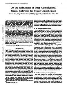
Figure 1. Quotes from four different market participants (sources) for the same CDS2 throughout one day. Each trader displays from time to time the prices for which he offers to buy (bid) and sell (ask) the underlying CDS. The filled area marks the difference between the best sell and buy offers (spread) at each time.

Imperial College London, London, United Kingdom Hellebore Capital Ltd., London, United Kingdom 3 Ecole Polytechnique, Palaiseau, France. Correspondence to: Mikołaj Bi´nkowski .

A common situation with financial data is that the same signal (e.g. value of an asset) is observed from different sources (e.g. financial news, analysts, portfolio managers in hedge funds, market-makers in investment banks) in asynchronous moments of time. Each of these sources may have a different bias and noise with respect to the orig-

Under review by the International Conference on Machine Learning (ICML). Do not distribute.

2 iTraxx Europe Main Index, a tradable Credit Default Swap index of 125 investment grade rated European entities.

1

2

Autoregressive Convolutional Neural Networks for Asynchronous Time Series

inal signal that needs to be recovered (cf. time series in Figure 1). Moreover, these sources are usually strongly correlated and lead-lag relationships are possible (e.g. a marketmaker with more clients can update its view more frequently and precisely than one with fewer clients). Therefore, the significance of each of the available past observations might be dependent on some other factors that can change in time. Hence, the traditional econometric models such as AR, VAR, VARMA (Hamilton, 1994) might not be sufficient. Yet their relatively good performance motivates coupling such linear models with deep neural networks that are capable of learning highly nonlinear relationships. For these reasons, we propose Significance-Offset Convolutional Neural Network, a CNN-extension of standard autoregressive models (Sims, 1972; 1980) equipped with a nonlinear weighting mechanism and provide empirical evidence on its competitiveness with standard multilayer CNN and recurrent Long-Short Term Memory network (Hochreiter & Schmidhuber, 1997). The mechanism is inspired by the gating systems that proved successful in recurrent neural networks ((Hochreiter & Schmidhuber, 1997; Chung et al., 2014)) and highway networks ((Srivastava et al., 2015)).

2. Related work 2.1. Time series forecasting Literature in time series forecasting is rich, and has a long history in the field of econometrics which makes extensive use of linear stochastic models such as AR, ARIMA and GARCH processes to mention a few. Unlike in machine learning, research in econometrics is more focused on explaining variables rather than improving out-of-sample prediction power. In practice, one can notice that these models ‘over-fit’ on financial time series: their parameters are unstable and out-of-sample performance is poor. Reading through recent proceedings of the main machine learning venues (e.g. ICML, NIPS, AISTATS, UAI), one can notice that time series are often forecast using Gaussian processes (Petelin et al., 2011; Tobar et al., 2015; Hwang et al., 2016), especially when time series are irregularly sampled (Cunningham et al., 2012; Li & Marlin, 2016). Though still largely independent, researchers have started to “bring together the machine learning and econometrics communities” by building on top of their respective fundamental models yielding to, for example, the Gaussian Copula Process Volatility model (Wilson & Ghahramani, 2010). Our paper is in line with this emerging trend by coupling AR models and neural networks. Over the past 5 years, deep learning models have surpassed results from most of the existing literature in many fields (Schmidhuber, 2015): computer vision (Krizhevsky et al.,

2012), audio signal processing and speech recognition (Sak et al., 2014), natural language processing (NLP) (Bengio et al., 2003; Collobert & Weston, 2008; Grave et al., 2016; Jozefowicz et al., 2016). Although sequence modeling in NLP, i.e. prediction of the next character or word, is related to our forecasting problem (1), the nature of the sequences is too dissimilar to allow using the same cost functions and architectures. Literature on deep learning for time series forecasting is still scarce (cf. (Gamboa, 2017) for a recent review). Literature on deep learning for financial time series forecasting is even scarcer though interest in using neural networks for financial predictions is not new (Mozer, 1993; McNelis, 2005). Besides claims of secretive hedge funds (it can be marketing surfing on the deep learning hype), no promising results or innovative architectures were publicly published so far, to the best of our knowledge. In this paper, we investigate the gold standard architectures’ (CNNs, LSTMs) capabilities on AR-like artificial asynchronous and noisy time series, and on real financial data from the credit default swap market where some inefficiencies may exist, i.e. time series may not be totally random. 2.2. Gating mechanisms Gating mechanisms for neural networks were first proposed by (Hochreiter & Schmidhuber, 1997) and proved essential in training recurrent architectures (Jozefowicz et al., 2016) due to their ability to overcome the vanishing gradient problem. In general, they can be expressed as f (x) = c(x) ⊗ σ(x),

(2)

where f is the output function, c is a ‘candidate output’ (usually a nonlinear function of x), ⊗ is an element-wise matrix product and σ : R → [0, 1] is a sigmoid nonlinearity that controls the amount of the output passed to the next layer (or to further operations within a layer). Appropriate compositions of functions of type 2 lead to the common recurrent architectures such as LSTM (Hochreiter & Schmidhuber, 1997) and GRU (Chung et al., 2014). A similar idea was recently used in construction of highway networks (Srivastava et al., 2015) which enabled successful training of deeper architectures. (van den Oord et al., 2016) and (Dauphin et al., 2016) proposed gating mechanisms (respectively with hyperbolic tangent and linear ‘candidate outputs’) for training deep convolutional neural networks. The gating system that we propose is aimed at weighting a number of different ‘candidate predictors’ and therefore is most closely related to the softmax3 gating used in MuFuRU (Multi-Function Recurrent Unit, (Weissenborn & 3

See Equation (13).

Autoregressive Convolutional Neural Networks for Asynchronous Time Series

Rockt¨aschel, 2016)), i.e. f (x) =

L X

pl (x) ⊗ f l (x),

p(x) = softmax(b p(x)), (3)

l=1

where (f l )L l=1 are candidate outputs (composition operators in MuFuRu) and (b pl )L l=1 are linear functions of the inputs.

3. Model Architecture Suppose that we are given a multivariate time series (xt )t ⊂ Rd and we aim to predict the conditional future values of a subset of elements of xt yt = E[xIt |{xt−i , i = 1, 2, . . .}],

(4)

where I = {i1 , i2 , . . . idI } ⊂ {1, 2, . . . , d} is a subset of features of xt . Let x−N = (xt−n )N t n=1 . We consider the following estimator of yt (j)

yˆt

=

M X   F (x−N ) ⊗ σ(S(x−N )) jm , j ∈ 1, 2, . . . , dI , t t m=1

(5) where • F, S : Rd×N → RdI ×M are neural networks, • σ is a normalized activation function independent on each row, i.e. σ((aT1 , . . . , aTM )T ) = (σ(a1 )T , . . . , σ(aN )T )T (6) for any a1 , . . . , aN ∈ RM and some σ such that 1T σ(a) = 1 for any a ∈ RM .

Figure 2. A scheme of proposed SOCNN architecture. The network preserves the time-dimension up to the last layer, while the number of features per timestep (filters) in the hidden layers is custom. The last convolutional layer, however, has the number of filters equal to the output dimension. The offset layer learns individual features for each observation through 1x1 convolutions.

• ⊗ is Hadamard (element-wise) matrix multiplication. It is easy to see that j-th element of the output vector yˆt is a linear combination of the the j-th row of matrix F (x−N ). t Consider now the special case when M = N , S is a convolutional neural network (composed solely of convolutional layers) and F is of the form  N F (x−N ) = W ⊗ off(xt−n ) + xIt−n ) n=1 (7) t where W ∈ RdI ×N and off : Rd → RdI is a multilayer perceptron. In that case F can be seen as a sum of projection (x 7→ [xin ]i∈I,n=1,...,N ) and a convolutional network with all convolution kernels of length 1. Equation (5) can be rewritten as

We will call the proposed network a Significance-Offset Convolutional Neural Network (SOCNN), off and S are respectively the offset and significance sub-networks. The network scheme is shown in Figure 2. Note that the form of Equation (8) enforces the separation of temporal dependence (obtained in weights Wn ), the local significance of observations Sn (S as a convolutional network is determined by its filters which capture local dependencies and are independent on the relative position in time) and the predictors off(xt−n ) that are completely independent on position in time. This provides some amount of interpretability of the fitted functions and weights.

Wn ⊗ (off(xt−n ) + xIt−n ) ⊗ σ(Sn (x−N )), (8) t

For instance, each of the past observations provides a single estimate of the target variable through the offset network.

where Wn , Sn (·)n are n-th columns of matrices W and S(·).

Note that when off ≡ 0 and σ ≡ 1 the model simplifies to the collection of dI separate AR(N ) models for each dimension.

yˆt =

N X n=1

Autoregressive Convolutional Neural Networks for Asynchronous Time Series

Loss function

V\QFKURQRXVGDWDVHW[.



2

L error is a natural loss function for the estimators of expected value 2

0

0 2

L (y, y ) = ky − y k .

(9)













As mentioned above, the output of the offset network can be seen as a collection of separate predictors of the changes between corresponding observations xIt−n and the target variable yt off(xt−n ) ' yt − xIt−n . (10) For that reason, we consider the auxiliary loss function equal to mean squared error of such intermediate predictions aux

L

(x−N t , yt )

N 1 X koff(xt−n )+xIt−n −yt k2 . (11) = N n=1

The total loss for the sample (x−N , yt ) is therefore given t by 2 Ltot (x−N yt , yt ) + αLaux (x−N t , yt ) = L (b t , yt ),

(12)

where ybt is given by Eq. 8 and α ≥ 0 is a constant. In Section 4.5 we discuss the empirical findings on the impact of positive values of α on the model training and performance, as compared to α = 0 (lack of auxiliary loss). Weighting activation We consider two types of activations σ, the softmax activation !M exp(xm ) sof tmax σ (x) = PM , (13) 0 m0 =1 exp(xm ) m=1 and the following normalized softplus activation !M log(1 + exp(x )) m . (14) σ ns+ (x) = PM 0 m0 =1 log(1 + exp(xm )) m=1

4. Experiments We evaluate the proposed model on a financial dataset of bid/ask quotes sent by several market participants active in the credit derivatives market and artificial datasets, comparing its performance with deep Convolutional Neural Network and Long-Short Term Memory network (Hochreiter & Schmidhuber, 1997) as most of successful neural network models for many other sequential datasets descend from these architectures. Apart from performance evaluation of SOCNNs, we discuss the impact of the network components, such as auxiliary loss and the depth of the offset sub-network.

VRXUFH% VRXUFH& VRXUFH)

VRXUFH/ VRXUFH1 VRXUFH2

 VRXUFH% VRXUFH& VRXUFH)

 

DV\QFKURQRXVGDWDVHW[.









VRXUFH/ VRXUFH1 VRXUFH2 







WLPHVWHSV

















WLPHVWHSV

Figure 3. Simulated synchronous (left) and asynchronous (right) artificial series. Note the different durations between the observations from different sources in the latter plot. For clarity, we present only 6 out of 16 total dimensions.

4.1. Datasets Artificial data We test our network architecture on the artificially generated datasets of multivariate time series. We consider two types of series: 1. Synchronous series. The series of K noisy copies (‘sources’) of the same univariate autoregressive series (‘base series’), observed together at random times. The noise of each copy is of different type. 2. Asynchronous series. The series of observations of one of the sources in the above dataset. At each time, the source is selected randomly and its value at this time is added to form a new univariate series. The final series is composed of this series, the durations between random times and the indicators of the ‘available source’ at each time. The details of the simulation process are presented in Appendix A4 . We consider synchronous and asynchronous series XK×N where K ∈ {16, 64} is the number of sources and N ∈ {10, 000, 100, 000}, which gives 8 artificial series in total. Note that a series with K sources is K + 1dimensional in synchronous case and K + 2-dimensional in asynchronous case. The base series in all processes was a stationary AR(10) series. Although the series have the true order of 10, in the experimental setting the input data included past 60 observations. The rationale behind that is twofold: not only is the data observed in irregular random times but also in real-life problems the order of the model is unknown. Figure 3 presents samples from two of the simulated series. Non-anonymous quotes The proposed model was designed primarily for forecast4

The code for simulation as well as the simulated processes used for model evaluation are available online at https://github.com/mbinkowski/nntimeseries.

Autoregressive Convolutional Neural Networks for Asynchronous Time Series

ing incoming non-anonymous quotes received from the credit default swap market. The dataset contains 2.1 million quotes from 28 different sources, i.e. market participants. Each quote is characterized by 31 features: the offered price, 28 indicators of the quoting source, the direction indicator (the quote refers to either a buy or a sell offer) and duration from the previous quote. For each source and direction we aim at predicting the next quoted price from this given source and direction considering the last 100 quotes. This dataset, which is proprietary, motivated the aforementioned construction of artificial asynchronous time series datasets based on its statistical features for reproducible research purpose. 4.2. Network settings To evaluate the model and the significance of its components, we perform a grid search over some of the hyperparameters, more extensively on the artificial datasets. These include the offset sub-network’s depth, the auxiliary weight α and the weighting activation σ. Table 1 provides a summary of the tested values. We have chosen LeakyReLU Artificial datasets

parameter offset depth aux. weight (α) weight activation (σ)

Quotes dataset

{1, 2, 5, 10} {2, 7} {0, 0.01, 0.1} {0.1} Softmax Normalized Softplus5

Table 1. The hyperparameters of SOCNN tested in grid search.

each trained CNN, we applied max pooling with the pool size of 2 every two convolutional layers (hence layers 3, 6 and 9 were pooling layers, while layers 1, 2, 4, 5, . . . were convolutional layers). Table 2 presents the configurations of the network classes used in comparison. Artificial Datasets Model layers SOCNN10+10 10conv + 10conv1 SOCNN10+5 10conv + 5conv1 SOCNN10+2 10conv + 2conv1 SOCNN10+1 10conv + 1conv1

f

ks

16

1 / (3, 1) / 3

7conv + 3pooling

32 16

(3, 1) / 3

1lstm 1lstm

64 32

layers 7conv + 7conv1

f 8

ks 1 / (3, 1)

CNN7x16

7conv + 3pooling

32

(3, 1) / 3

LSTM32

1lstm

32

CNN10x32 CNN10x16 LSTM64 LSTM32 Quotes Dataset Model SOCNN7+7

Table 2. Configurations of the trained models. f - number of convolutional filters/memory cell size in LSTM, ks - kernel size, conv - (k × 1) convolution with kernel size k indicated in the last column, conv1 - (1 × 1) convolution. Apart from the listed layers, each network has a single fully connected layer on the top. Kernel size (3, 1) denotes alternating kernel sizes 3 and 1 in successive convolutional layers.

activation function (15) σ

LeakyReLU

 (x) =

x, ax,

x ≥ 0, x < 0,

(15)

with leak rate a = .1 as an activation function in the intermediate convolutional layers. 4.3. Benchmark networks We compare the performance of the proposed model with Convolutional Neural Network (CNN) and Long-Short Term Memory (LSTM) network. The benchmark networks were designed so that they have a comparable number of parameters as the proposed model. Consequently, LeakyReLU activation function (15) with leak rate .1 was used in all layers except the top ones where linear activation was applied. Additionally, for CNN we provided the same number of layers, same stride (1) and similar kernel size structure. In 5

See Equation (14).

4.4. Network Training Each of the series was split into separate training set (first 80% of the steps) and validation set (last 20% of data). All models were trained using Adam optimizer ((Kingma & Ba, 2015)) which we found much faster than standard Stochastic Gradient Descent in early tests. We used batch size of 128 for artificial data and 8 for quotes dataset (for the latter we found smaller batch size beneficial across all models). We also applied batch normalization (Ioffe & Szegedy, 2015) in between each convolution and the following activation. At the beginning of each epoch, the training samples were shuffled. The initial learning rate was set to .001 for artificial data and .0003 for quotes data. We applied early stopping to prevent overfitting in the following way; whenever 5 consecutive epochs did not bring improvement in the validation error, the learning rate was reduced by a factor of 10 and the best weights obtained till then were restored.

Autoregressive Convolutional Neural Networks for Asynchronous Time Series

Experiments were carried out using implementation relying on Tensorflow (Abadi et al., 2016) and Keras backend (Chollet, 2015). For artificial data we optimized the models using 1 K20s NVIDIA GPU while for quotes dataset we used 8-core Intel Core i7-6700 CPU machine only. 4.5. Results Table 3 presents the detailed results from the artificial datasets. The proposed networks outperform significantly the benchmark networks on the asynchronous datasets. For the synchronous datasets, on the other hand, SOCNN almost matches the results of traditional CNN; both of the architectures performed considerably better than LSTM. We can also observe that the depth of the offset network has negligible impact on the overall performance of the SOCNN network, especially for datasets with higher amount of samples.

VRXUFH

In Figure 4, we display results from the quotes dataset. It shows the predictability of market participants: some are rather unpredictable (e.g. the ones who are the fastest to integrate new pieces of information), some others are rather predictable (maybe those with a smaller market share who have access to less feedback from their counterparties and thus update their views with some lag, yet non-deterministically) and some are almost perfectly predictable (perhaps quoting robots updating their prices according to a basic and fixed algorithm). Notice that all models agree on the predictability of the sources.

62&11 &11 /670 9$5

$ % & ' ( ) * + , . / 



Since all of SOCNN networks achieved comparable results for each of the datasets, we group them together in the following analysis. Table 4 presents the impact of the auxiliary loss weight on the validation error. It can be observed that positive values of α led to significantly lower validation errors for asynchronous datasets. Overall, α > 0 were chosen6 for 23 out of 32 of model/dataset configurations, with values 0.1 more frequent for asynchronous datasets and 0.01 for synchronous ones. We also observed that softmax was chosen roughly twice more often than the proposed normalised softplus as the best weighting activation. 6\QFKURQRXV[.



62&11α = 0 62&11α = 0. 1 &11 &11

   

62&11α = 0 62&11α = 0. 01 &11 &11



PHDQVTXDUHGHUURU

Weights were initialized following the normalized uniform procedure proposed by (Glorot & Bengio, 2010).

Impact of Auxiliary Loss

PHDQVTXDUHGHUURU

After the third reduction and another 5 consecutive epochs without improvement, the training was stopped.

     



















WLPHVHFRQGV













HSRFK

Figure 5. Learning curves for CNNs and SOCNNs with different auxiliary weights for two different artificial datasets. The solid lines indicate the validation error while the dashed lines indicate the training error. Note the different scales on the horizontal axes in the plots: in the left one, the error evolution is aligned with training time, while in the right one with training epochs.

The auxiliary weight helped achieve more stable validation error throughout training in many cases. In general, the proposed SOCNN had significantly lower variance of the validation error, especially in the early stage of the training process. Figure 5 presents the learning curves for two different artificial datasets.

5. Conclusion and discussion In this article, we proposed a weighting mechanism that, coupled with convolutional networks, forms a new neural network architecture for time series prediction. The proposed architecture is designed for regression tasks on asynchronous signals in the presence of high amount of noise. This approach has proved to be successful in forecasting financial and artificially generated asynchronous time series outperforming both plain convolutional and LSTM networks. 









PHDQVTXDUHGHUURU

Figure 4. Results for the quotes dataset. The plot presents the validation out-of-sample error for 12 significant market participants.

The proposed model can be further extended by adding intermediate weighting layers of the same type in the network structure. Another possible generalization that requires fur6 In the grid search of all hyperparameters listed in Table 1 for all of the SOCNN models presented in 2.

Autoregressive Convolutional Neural Networks for Asynchronous Time Series

model SOCNN10+1 SOCNN10+2 SOCNN10+5 SOCNN10+10 CNN10x16 CNN10x32 LSTM32 LSTM64

16x100K 0.1838 (0.1840) 0.1830 (0.1843) 0.1837 (0.1845) 0.1863 (0.1879) 0.1830 (0.1835) 0.1832 (0.1842) 0.1941 (0.1941) 0.2049 (0.2049)

type 1 (Synchronous) 64x100K 16x10K 0.0498 0.1604 (0.0498) (0.1628) 0.0498 0.1608 (0.0500) (0.1634) 0.0498 0.1662 (0.0500) (0.1680) 0.0506 0.1629 (0.0507) (0.1696) 0.0495 0.1605 (0.0496) (0.1629) 0.0496 0.1602 (0.0496) (0.1634) 0.0825 0.2127 (0.0825) (0.2127) 0.0773 0.2257 (0.0773) (0.2257)

64x10K 0.0456 (0.0470) 0.0449 (0.0461) 0.0467 (0.0518) 0.0493 (0.0504) 0.0447 (0.0454) 0.0445 (0.0453) 0.2369 (0.2369) 0.6260 (0.6260)

16x100K 0.0139 (0.0140) 0.0140 (0.0144) 0.0139 (0.0143) 0.0139 (0.0142) 0.0238 (0.0244) 0.0242 (0.0253) 0.0750 (0.0750) 0.0668 (0.0668)

type 2 (Asynchronous) 64x100K 16x10K 0.0165 0.0167 (0.0166) (0.0186) 0.0168 0.0183 (0.0173) (0.0201) 0.0167 0.0172 (0.0174) (0.0203) 0.0166 0.0184 (0.0167) (0.1432) 0.0177 0.0403 (0.0181) (0.0507) 0.0179 0.0395 (0.0184) (0.0490) (0.0273) 0.2782 (0.0273) (0.2782) 0.0346 0.4178 (0.0346) (0.4178)

64x10K 0.0255 (0.0485) 0.0266 (0.0426) 0.0270 (0.0315) 0.0227 (0.0521) 0.0451 (0.0851) 0.0396 (0.0598) 0.3290 (0.3290) 0.1295 (0.1295)

Table 3. Detailed results for artificial datasets. For each model, the first line represents the lowest out-of-sample mean squared error, while the second (with numbers in parentheses) shows the average of out-of-sample errors obtained in 4 independent runs of the training process in the best setting. The best results for each dataset are marked by bold font.

SOCNN

CNN LSTM

α 0 0.01 0.1 – –

Synchronous 101.80% 105.78% 109.63% 101.47% 135.74%

Asynchronous 160.21% 120.40% 119.89% 243.14% 345.63%

Table 4. The average normalized mean squared error for different auxiliary weights α. 100% = mean squared error for the best model for each dataset.

ther empirical studies can be obtained by leaving the assumption of independent offset values for each past observation, i.e. considering not only 1x1 convolutional kernels in the offset sub-network. Finally, we aim at testing the performance of the proposed architecture on other real-life datasets with relevant characteristics. We observe that there exists a strong need for common ‘econometric’ datasets benchmark and, more generally, for time series (stochastic processes) regression.

6. Acknowledgements Authors would like to thank Hellebore Capital Ltd. for providing data for the experiments. M.B. thanks Engineering and Physical Sciences Research Council (EPSRC) for partial funding of this research.

References Abadi, Mart´ın, Barham, Paul, Chen, Jianmin, Chen, Zhifeng, Davis, Andy, Dean, Jeffrey, Devin, Matthieu, Ghemawat, Sanjay, Irving, Geoffrey, Isard, Michael, Kudlur, Manjunath, Levenberg, Josh, Monga, Rajat, Moore, Sherry, Murray, Derek G., Steiner, Benoit, Tucker, Paul, Vasudevan, Vijay, Warden, Pete, Wicke, Martin, Yu, Yuan, and Zheng, Xiaoqiang. TensorFlow: A system for large-scale machine learning, May 2016. URL http://arxiv.org/abs/1605.08695. Bengio, Yoshua, Ducharme, R´ejean, Vincent, Pascal, and Janvin, Christian. A neural probabilistic language model. J. Mach. Learn. Res., 3:1137–1155, March 2003. ISSN 1532-4435. URL http://portal. acm.org/citation.cfm?id=944966. Bun, Jo¨el, Bouchaud, Jean-Philippe, and Potters, Marc. Cleaning large correlation matrices: tools from random matrix theory. Physics Reports, 666:1–109, 2017. Chollet, Franc¸ois. Keras. https://github.com/ fchollet/keras, 2015. Chung, Junyoung, Gulcehre, Caglar, Cho, KyungHyun, and Bengio, Yoshua. Empirical evaluation of gated recurrent neural networks on sequence modeling, December 2014. URL http://arxiv.org/abs/1412. 3555.

Autoregressive Convolutional Neural Networks for Asynchronous Time Series

Collobert, Ronan and Weston, Jason. A unified architecture for natural language processing: Deep neural networks with multitask learning. In Proceedings of the 25th international conference on Machine learning, pp. 160–167. ACM, 2008. Cont, Rama. Empirical properties of asset returns: stylized facts and statistical issues. Quantitative Finance, 1(2): 223–236, 2001. Cunningham, John P, Ghahramani, Zoubin, Rasmussen, Carl Edward, Lawrence, ND, and Girolami, M. Gaussian processes for time-marked time-series data. In AISTATS, volume 22, pp. 255–263, 2012.

Jozefowicz, Rafal, Vinyals, Oriol, Schuster, Mike, Shazeer, Noam, and Wu, Yonghui. Exploring the limits of language modeling, February 2016. URL http:// arxiv.org/abs/1602.02410.pdf. Kingma, Diederik and Ba, Jimmy. Adam: A method for stochastic optimization. January 2015. URL http: //arxiv.org/abs/1412.6980. Krizhevsky, Alex, Sutskever, Ilya, and Hinton, Geoffrey E. Imagenet classification with deep convolutional neural networks. In Advances in neural information processing systems, pp. 1097–1105, 2012.

Dauphin, Yann N., Fan, Angela, Auli, Michael, and Grangier, David. Language modeling with gated convolutional networks, December 2016. URL http://arxiv. org/abs/1612.08083.pdf.

Laloux, Laurent, Cizeau, Pierre, Potters, Marc, and Bouchaud, Jean-Philippe. Random matrix theory and financial correlations. International Journal of Theoretical and Applied Finance, 3(03):391–397, 2000.

Fama, Eugene F. Efficient capital markets: A review of theory and empirical work. The journal of Finance, 25 (2):383–417, 1970.

Lecun, Y., Bottou, L., Bengio, Y., and Haffner, P. Gradientbased learning applied to document recognition. Proceedings of the IEEE, 86(11):2278–2324, November 1998. ISSN 00189219. doi: 10.1109/5.726791. URL http://dx.doi.org/10.1109/5.726791.

Gamboa, John Cristian Borges. Deep learning for timeseries analysis. arXiv preprint arXiv:1701.01887, 2017. Glorot, Xavier and Bengio, Yoshua. Understanding the difficulty of training deep feedforward neural networks. In In Proceedings of the International Conference on Artificial Intelligence and Statistics (AISTATSˆa10). Society for Artificial Intelligence and Statistics, 2010. URL http://citeseerx.ist.psu.edu/viewdoc/ summary?doi=10.1.1.207.2059. Grave, Edouard, Joulin, Armand, Ciss´e, Moustapha, Grangier, David, and J´egou, Herv´e. Efficient softmax approximation for GPUs, December 2016. URL http: //arxiv.org/abs/1609.04309.pdf. Hamilton, James Douglas. Time series analysis, volume 2. Princeton university press Princeton, 1994. Hochreiter, Sepp and Schmidhuber, J¨urgen. Long ShortTerm memory. Neural Computation, 9(8):1735–1780, November 1997. ISSN 0899-7667. doi: 10.1162/ neco.1997.9.8.1735. URL http://dx.doi.org/ 10.1162/neco.1997.9.8.1735. Hwang, Yunseong, Tong, Anh, and Choi, Jaesik. Automatic construction of nonparametric relational regression models for multiple time series. In Proceedings of the 33rd International Conference on Machine Learning, 2016. Ioffe, Sergey and Szegedy, Christian. Batch normalization: Accelerating deep network training by reducing internal covariate shift, March 2015. URL http://arxiv. org/abs/1502.03167v2.pdf.

Li, Steven Cheng-Xian and Marlin, Benjamin M. A scalable end-to-end gaussian process adapter for irregularly sampled time series classification. In Advances in Neural Information Processing Systems, pp. 1804–1812, 2016. McNelis, Paul D. Neural networks in finance: gaining predictive edge in the market. Academic Press, 2005. Mozer, Michael C. Neural net architectures for temporal sequence processing. In Santa Fe Institute Studies in the Sciences of Complexity, volume 15, pp. 243–243, 1993. ˇ Petelin, Dejan, Sindel´ aˇr, Jan, Pˇrikryl, Jan, and Kocijan, Juˇs. Financial modeling using gaussian process models. In Intelligent Data Acquisition and Advanced Computing Systems (IDAACS), 2011 IEEE 6th International Conference on, volume 2, pp. 672–677. IEEE, 2011. Sak, Hasim, Senior, Andrew W, and Beaufays, Franc¸oise. Long short-term memory recurrent neural network architectures for large scale acoustic modeling. In Interspeech, pp. 338–342, 2014. Schmidhuber, J¨urgen. Deep learning in neural networks: An overview. Neural networks, 61:85–117, 2015. Sims, Christopher A. Money, income, and causality. The American economic review, 62(4):540–552, 1972. Sims, Christopher A. Macroeconomics and reality. Econometrica: Journal of the Econometric Society, pp. 1–48, 1980.

Autoregressive Convolutional Neural Networks for Asynchronous Time Series

Srivastava, Rupesh K., Greff, Klaus, and Schmidhuber, J¨urgen. Highway networks, November 2015. URL http://arxiv.org/abs/1505.00387. Tobar, Felipe, Bui, Thang D, and Turner, Richard E. Learning stationary time series using gaussian processes with nonparametric kernels. In Advances in Neural Information Processing Systems, pp. 3501–3509, 2015. van den Oord, Aaron, Kalchbrenner, Nal, Vinyals, Oriol, Espeholt, Lasse, Graves, Alex, and Kavukcuoglu, Koray. Conditional image generation with PixelCNN decoders, June 2016. URL http://arxiv.org/abs/1606. 05328. Weissenborn, Dirk and Rockt¨aschel, Tim. MuFuRU: The Multi-Function recurrent unit, June 2016. URL http: //arxiv.org/abs/1606.03002v1.pdf. Wilson, Andrew and Ghahramani, Zoubin. Copula processes. In Advances in Neural Information Processing Systems, pp. 2460–2468, 2010.

A. Artificial data generation We simulate a multivariate time series composed of K noisy observations of the same autoregressive signal. The simulated series are constructed as follows: 1. We simulate univariate stationary AR(10) time series x with randomly chosen weights. 2. The series is copied K times and each copy x(k) is associated with a separate noise process ε(k) . We consider Gaussian or Binomial noise of different scales; for each copy it is either added to or multiplied by the initial series (x(k) = x + ε(k) or x(k) = x × ε(k) ). 3. We simulate a random time process T where differences between consecutive events are iid exponential random variables. 4a. The final series is composed of K noisy copies of the original process observed at times indicated by the random time process, and a duration between observations. 4b. At each time T (t) indicated by the random time process T , one of the noisy copies k is drawn and its value (k) at this time xT (t) is selected to form a new noisy se∗ ries x . The final multivariate series is composed of x∗ , the series of durations between observations and K indicators of which observation was drawn at each time.

Assume that (xt )t=1,2,... is a stationary AR(ν) series and consider the following (random) noise functions ε0 (x, c, p) = x + c(2 − 1),

 ∼ Bernoulli(p),

ε1 (x, c, p) = x(1 + c(2 − 1)),

 ∼ Bernoulli(p),

ε2 (x, c, p) = x + c,

 ∼ N (0, 1),

ε3 (x, c, p) = x(1 + c),

 ∼ N (0, 1). (16)

Note that argument p of ε2 and ε3 is redundant and was added just for notational convenience. Let Nt ∼ Exp(λ) be a series of i.i.d. exponential random variables with some constant rate λ and let T (t) = P t s=1 dNs + 1e. Then T (t) is a strictly increasing series of times, at which we will observe the noisy observations. Let p1 , p2 , . . . , pK ∈ (0, 1) and define  εk(mod 4) (xT (t) , 2−bk/8c , pk ), (k) Xt := T (t),

k = 1, . . . , K, k = K + 1. (17) Let I(t) be a series of i.i.d. random variables taking values in {1, 2, . . . , K} such that P(I(t) = K) ∝ q K for some q > 0. Define  1, k ≤ K and k = I(t),    0, k ≤ K and k 6= I(t), (k) ¯ t := (18) X (I(t))  X , k = K + 1,   t T (t), k = K + 2. ¯ N We call {Xt }N t=1 and {Xt }t=1 synchronous and asynchronous time series, respectively. We simulate both of the processes for each N ∈ {10, 000, 100, 000} and K ∈ {16, 64}.