Dec 10, 1998 - Bayesian analysis of autoregressive moving average models is dis- cussed with di ... Model selection is a also discussed through the use of the.
Autoregressive moving average models with t and hyperbolic innovations December 10, 1998
Wolfgang Polasek
Institute of Statistics and Econometrics 4051 Basel University of Basel Switzerland
Je rey Pai
Warren Centre for Actuarial Studies and Research University of Manitoba Canada
Abstract
Bayesian analysis of autoregressive moving average models is discussed with di�erent distributional assumptions for the noise process. The proposed Gaussian white noise is a mixture distribution where the hyper-parameter follows two di�erent hyper-distributions to incorporate, the t distribution and the hyperbolic distribution. The Metropolis-Hastings and Gibbs sampler are used for the Bayesian estimation. Model selection is a also discussed through the use of the predictive distribution, pseudo-marginal likelihoods and pseudo-Bayes factors. The models are estimated for daily and monthly exchange rates (SFr./US$).
: ARMA processes, leptokurtic returns, t and hyperbolic distributions, MCMC methods, CPO plots, pseudo-marginal likelihood.
Keywords
: We thank Lei Ren for the computation of the models which are provided in the BASEL package. More information can be obtained from http : ==www:unibas:ch=iso=basel=basel:html.
Acknowledgment
1
1 Introduction Recent research in empirical nance has shown renewed interests in the distributional properties of returns of securities since the pricing of derivatives depends heavily on distributional assumptions. The phenomenon of leptokurtic distributions of "speculative prices" has been known since Mandelbrot (1963) and Fama (1965), and econometric approaches to model leptokurtosis have produced only moderate success. The use of ARCH (autoregressive conditional heteroskdastic) models which were introduced by Engle (1982) is popular for modeling volatility clusters, but it could not resolve the puzzle of the 'right' distributional assumptions. Many empirical studies for nancial time series have shown that the usual ('normal') Gaussian distributional assumptions are not adequate. For nancial time series it is reasonable to assume that the underlying distribution has heavier tails, for example a t distribution with low degrees of freedom. The hyperbolic distribution was suggested by Barndor�-Nielsen et al. (1985) as an alternative distribution when there is considerably more mass around the origin and in the tails than in the standard normal distribution. Engle (1980) expressed this kind of behavior as leptokurtosis which is very important in modeling nancial data. Eberlein and Keller (1995) applied the class of hyperbolic distributions and improved the tness to the empirical returns. Recently, Barndor�-Nielsen (1997) has suggested to use the normal inverse Gaussian distribution for stochastic processes in nance and stochastic volatility modeling. Both, the t distribution and the hyperbolic distribution can be considered as a mixture of normal distributions. These results are conceptually straightforward in Bayesian analysis. Consider a normal distribution with variance �2 for the error term �, i.e. � N (0� �2): Using �2 as a hyper-parameter in a scale mixture of normal distributions, we can get the t distribution and the hyperbolic distribution by mixing (see Appendix C). From the Bayesian point of view, the idea of mixing is formulated in a hierarchical model and the posterior distribution of all the parameters of the model will be numerically simulated by Markov chain Monte Carlo (MCMC) methods. In Section 2 we start with the likelihood for the normal ARMA(p,q) model 2
and we derive all the complete conditional densities for the parameters of the t-ARMA and the hyp-ARMA model. We specify hyper-distribution on the variance of the Gaussian white noise distribution to arrive at t distribution and hyperbolic distribution. Model choice and MCMC methods like the Gibbs sampler and the MetropolisHastings algorithm are explained in Section 3. The predictive density is discussed in Section 4. We study the CPO (conditional predictive ordinate) plots and the pseudo Bayes factors to select the best model. Since we have assumed for some parameters a non-informative prior distribution, we use the approach of Gelfand and Dey (1994) to calculate pseudo Bayes factors. In Section 5 we illustrate our models with exchange rate data (SFr./US$ from June 1973 to May 1984). In Section 6 we nish with some conclusions. In the appendix we discuss the generalized inverse Gaussian (GIG) distribution, the Bessel function and the hyperbolic distribution.
2 ARMA Processes Autoregressive moving average models constitute a broad class of parsimonious time series processes which are useful in describing a wide variety of time series (Box and Jenkins, 1976). The stochastic process fztg, t 2 Z is said to be an ARMA(p,q) process with mean � if it is generated by
�(B )(zt ; � ) = �(B )�t�
(1)
where B is the backshift operator Bzt = zt;1 and �(B ) = 1 ; �1B ;� � �; �pB p and �(B ) = 1 ; �1B ; � � � ; �q B q are lag polynomials in B of degrees p and q, respectively, and �t are independent and identically distributed random variables with mean 0 and variance �2.
2.1 The likelihood for the ARMA(p,q) model
Consider mean centered observations yt = zt ; � , then the ARMA(p,q) process in (1) can be written as
X X y = � y ; ; � � ; + � � t = 1� : : : � T: p
t
j =1
q
j t j
j =1
j t j
3
t
Let fn(zn jZn;1� �0) be the conditional density of the observation zn given all the observed time series values in Zn;1 up to time n ; 1 and the initial values �0. We denote the likelihood for n observations Zn = (z1� � � � � zn) by f (Zn ��) where the parameters are � = (�� �� �� �2) (2) with � = (�1� � � � � �p) and � = (�1� � � � � �q ): Our analysis is based on the conditional likelihood function where Z�0] = (z1;p� � � � � z0) and E�0] = (�1;q � � � � � �0) are the starting values. The initial values and parameters are given by �0 = (�� E�0]� Z�0]) and the likelihood function under normality (Gaussian distribution) can be written as f (Zn j�0) = f1(z1j�0)f2(z2jZP1� �0) � � � fn(znjZn;1 � �0) 2 (3) = (2��2); 2 exp�; (y2t �;2 �t) ] n
where the conditional means of the process are
�t =
X � y ; X � (y ; � ) + �: ; ; ; p
i=1
q
i t i
i
i=1
t i
t i
(4)
For the prior distribution we assume independent blocks, i.e. �(�) = �(�)�(�)�(�2)�(� )� (5) and we assume a di�use prior for the location parameters �(�) / 1� �(�) / 1� �(� ) / 1� and a conjugate inverse gamma (IG) distribution for the scale parameter �2 �(�2) = ;( ) �1(�2)� +1 exp(; �21 ):
The posterior distribution for � is proportional to the product of the likelihood (3) and the prior (5): �(�jZn� E�0]� Z�0]) / f (Zn j�� E�0]� Z�0])�(�) P(yt ; �t)2 2 ;2 (6) / (� ) exp�; 2�2 ]�(�): To apply the Gibbs-Metropolis sampler, we derive from the posterior distribution the so-called complete conditional distribution for blocks of parameters. n
4
The complete conditional densities (c.c.d.) for the ARMA(p,q) parameters � , �, and � is via (6) proportional to P(yt ; �t)2 �(�j� n �� Zn ) / exp�; 2�2 ]� (7) P(yt ; �t)2 (8) �(�j� n �� Zn ) / exp�; 2�2 ]� P(yt ; �t)2 �(� j� n �� Zn ) / exp�; 2�2 ]: (9) The c.c.d. for the residual variance �2 is again an inverse gamma distribution (10) �(�2j� n �2� Zn ) = IG( + n2 � 2 + P2 (y ; � )2 )� t t where � n � denotes the set of parameters in � without �, and similar for the other parameters in above c.c.d.'s. As alternative we could specify an informative (normal) prior for the ARMA(p,q) parameters in (5), i.e. �(�� �� � ) = Np���� �� ]Nq ���� �� ]N ��� � �2]� (11) where �� � ��� �� � �� � �� , and �2 are known hyper-parameters. For the informative case the c.c.d.'s in (7), (8), and (9) have to be multiplied by the normal distributions in (11): P(yt ; �t)2 �(�j� n �� Zn ) / expf; 2�2 g expf; 21 (� ; �� )0�� (� ; �� )g� P(yt ; �t)2 �(�j� n �� Zn) / expf; 2�2 g expf; 21 (� ; �� )0��(� ; �� )g� P(yt ; �t)2 �(� j� n �� Zn ) / expf; 2�2 g expf; 12 (� ; �� )2= �2g:
2.1.1 The ARMA(p,q) model with t distributed innovations
Suppose that, given the parameter 2, v 2=�2 has a 2 (or gamma) prior distribution with v degrees of freedom, i.e., (v )v=2exp�; v�2 22 ] : 2 2 �(� j ) = ;(v=2)2v=2 (�)v=2+1 5
By integrating �2 over the product of the normal distribution and the 2 distribution, we will get the innovations �= as a t distribution with v degrees of freedom (see Appendix C.1). The c.c.d.'s of � , �, � are the same as in (7) to (9) of the previous subsection and to estimate the t distribution with � degrees of freedom we have to extend the parameter vector in (2) to � = (�� �� �� �2� 2) and the remaining c.c.d.'s are (�2j� n �2� Zn � �0) IG( n +2 v � v P(y2 ; � )2 )� t t 2 ( 2j� n 2� Zn� �0) Ga( v=2 2+ � � v 2�+ 2��2 )� � where � and � are the known prior hyper-parameters for 2. If the degrees of freedom � of the t distribution is not known then we can extend the parameters set to �~ = (�� � ) and sample � from a discrete set of integers.
2.1.2 The ARMA(p,q) model with hyperbolic innovations
Suppose that �2 has a generalized inverse Gaussian (GIG) distribution (see Appendix A) of the form �2 �;21; 1 GIG(� = 1� = � = �;2 ; 1): (12) Then the marginal distribution of � has a hyperbolic distribution (Barndor�Nielsen et al., 1985). Now the parameters to be estimated for the hypARMA(p,q) model (1) are de ned by � = (�� �� �� �2� 2� �) and the MCMC algorithm takes the following form. The c.c.d.'s for � , �, � are given by (7), (8) and (9), of the previous section, respectively. The c.c.d.'s for �2, 2 and � can be found to be P(yt ; �t)2 � (�;2 ; 1)2 2 2 ;n �(� j� n � � Zn � �0) / (�) exp�; 2�2 ; 2 ; 2�2 2 ]� (13) and (�;2 ; 1)2 ; ]� �( 2j� n 2� Zn � �0) / ( )� exp�; � ; (14) 2 2� 2 2
�
(�;2;1)2
; 2 2 �2 ] : �(�j� n �� Zn � �0) / (�;2exp� ; 1)K (�;2 ; 1) 1
6
�
(15)
We use for the c.c.d. of � and � a normal distribution which is obtained by an iteration proposal given by
� N ��old� �2 ]� � N ��old� �2]: The mean �old = 0:4, �old = 0:0, and the variance �2 = 0:01, �2 = 0:01 are obtained iteratively from Metropolis runs (e.g. 3 times thousand runs). We calculate the mean and variance and repeat the iterative proposal until a satisfactory acceptance=rejection ratio is obtained.
3 Sampling based methods 3.1 Gibbs sampling
Bayesian inference proceeds by obtaining marginal posterior distributions of the components of � as well as summary features of these distributions. The Metropolis-Hastings algorithm is attractive in Bayesian inference since the marginal or joint posterior distributions are always available up to a multiplicative constant. The Gibbs sampler was introduced by Gelfand and Smith (1990) as a tool for carrying out Bayesian calculations and is a Markovian updating scheme that proceeds as follows. Suppose we partition � into k components (�1� �2� : : :� �k ): Let �i = �(�ijf�j gj6=i � Zn ) denote the complete conditional density (c.c.d.) of �. Given an arbitrary set of starting (0) (0) values (�(0) 1 � �2 � : : : � �k ), we draw �(1) 1 �(1) 2
(0) �1(�1j�(0) 2 � : : :� �k � Zn )� (0) (0) �2(�2j�(1) 1 � �3 � : : :� �k � Zn )�
and so on, up to �(1) k
(1) (1) �k (�k j�(1) 1 � �2 � : : :� �k;1 � Zn )�
completing one iteration. Thus, each variable is visited in the natural order and a cycle in this scheme requires k random variate generations. After i such iterations we would arrive at (�(1i)� �(2i)� : : : � �(ki)): Under very mild regularity conditions (see Gelfand and Smith (1990) or Tierney (1994)), this Markov chain converges to a stationary distribution for large i, i.e. (�(1i)� : : : � �(ki)) and 7
follows a distribution which is approximately the required posterior distribution �(�1� : : : � �k jZn): Importantly, each complete conditional distribution is proportional to the joint density f (Zn ��) ��(�).
3.2 Metropolis-Hastings Algorithm
The Markov chain Monte Carlo using the Metropolis-Hastings (M-H) algorithm is a general method for the simulation of stochastic processes having probability densities known up to a constant of proportionality. The Metropolis algorithm was originally developed by Metropolis et al. (1953) and has been widely used by physicists since. Hastings (1970) re ned the Metropolis algorithm and introduced to statisticians in Monte Carlo estimates. The idea of the M-H algorithm is to use a general transition kernel P (u� v) (based on P (vju)) and the property of reversibility to get the stationary associated with P (u� v). In the continuous case the property R P (distribution u� v)dv = 1 holds, while in the discrete case P (u� v) is called a transition matrix and the summation over the discrete states yields P P (u� v) = 1. The property of reversibility means that �(u)P (u� v) = �(v)P (v� u) and the equilibrium distribution associated with P (u� v) is �(u). The M-H algorithm is the Markov chain Monte Carlo method which uses this result to generate samples from the desired distribution. Let P (u� v) = (u� v)q(u� v) where u) )� (u� v) = min(1� ��((uv))qq((v� u� v) and q(u� v) is any transition kernel on the appropriate space. The P (u� v) satis es the reversibility condition as follows. Suppose �(v)q(v� u) < �(u)q(u� v), u) q(u� v) �(u)P (u� v) = �(u) ��((uv))qq((v� u� v) = �(v)q(v� u)� and u�v)q(v� u) �(v)P (v� u) = �(v) ��((uv))qq((v� u) = �(v)q(v� u): 8
Similarly, the reversibility condition is satis ed if �(v)q(v� u) > �(u)q(u� v). There are several possibilities for the choices of q(u� v) �e.g., Metropolis et al. 1953), Hastings (1970), M!uller (1994), Tanner (1993), Chib and Greenberg (1993), Tierney (1994)]. One possibility is to let q(u� v) = v ; u (Metropolis et al. 1953) where z = v ; u is a random increment. Let z be a symmetric univariate (or multivariate) distribution (e.g. normal, t or uniform) centered at the origin. The acceptance probability (u� v) is in this case (u� v) = min(1� ��((uv)) ): q(u� v) is called the probing distribution which lines up the target distribution. This choice is also called the "random walk" or "dependent" chain. Another choice of q(u� v) is called the "independent" chain �Hastings (1970), Tierney (1994)]. In this choice q(u� v) = q(v), ignoring the current state, behaves like an importance sampling density. The rst choice need to specify only the spread while the second choice needs both the location and the spread of the probing distribution. The probability that the process does not move from u is given by Z r(u) = 1 ; (u� v)q(u� v)dv:
4 Prediction and Model Choice
4.1 The conditional predictive ordinate (CPO)
In the following section we adopt the model choice approach of Gelfand and Dey (1994) for the time series models. If z = (z1� : : :� zn) denotes the observed sample then z(r) denotes the observed data set with r-th observation deleted, i.e. z(r) = (z1� : : :� zr;1� zr+1� : : :� zn). We call f (zr jz(r)) the cross-validation density and if this density is evaluated at the observed data it is called the conditional predictive ordinate (CPO) CPOr = f (Z = zrjz(r)): (16) The product over all CPOs is called pseudo-predictive density or pseudomarginal likelihoods f (z) for non-informative priors:
Y PsML = CPO n
n
r
r =1
9
Y = f (z jz( )): r =1
r
r
(17)
The ratio of the pseudo-marginal likelihoods for 2 models, say I and J , is called pseudo-Bayes factor (PsBF) PsML(I ) = f (zr jz(r)� I ) : PsBF = PsML (18) (J ) f (zr jz(r)� J ) In the case of time series observations we use the notation Z�n] = (z1;p� : : : � zn) and E�n] = (�1;q � : : :� �n): (19) The cross-validation density is simply the one step-ahead predictive density f (znjZ�n] ) and the pseudo-marginal likelihood is given by
PsML =
Y f (z jZ n
r =1
r
�r;1]
):
(20)
For two models I and J the pseudo-Bayes factor is given by PsML(I ) : (21) PsBF = PsML (J ) In the next section we show how the pseudo-marginal likelihood PsML can be calculated from the MCMC sample (�1� : : : � �L) of size L.
4.1.1 MCMC and pseudo-Bayes factors
In a Bayesian analysis, prediction for a future observation zF proceeds via the predictive density, f (zF jZn ) where Zn is the observed data of size n. In practice, the predictive density may be obtained in two ways. We can treat the future unknown observation, zF , as unknown parameters in the Gibbs sampler. Alternatively, the predictive density can be approximated from the MCMC sample of the posterior distribution as following:
f (zF jZn ) =
Z
f (zF jZn � �)�(�jZn)d�
L X 1 � L f (zF jZn � �j )� j =1
(22)
where �j , j = 1� � � � � L are the output of the Gibbs sampler. To obtain a sample of predictions from the density (22), for each �j we draw zF�j from 10
f (zF jZn � �j ) which is simply the well-known conditional likelihood. Using notation (19), the forecasting predictive density f (ztjZ�t;1]) can be written as R f (Z�t] j�)�(�)d� f (ztjZ�t;1]) = R f (Z j�)�(�)d� : (23) �t;1] After some transformations the conditional predictive density in (23) can be obtained from the MCMC output in the following way: R 1 = +1 f (z jZ� ;1]� ) � (�jZn )d� f (ztjZ�t;1]) = R 1 = f (z jZ� ;1] � ) � (�jZn )d� �Lj=1 = +1 f (z 1jZ� ;1]� ) : (24) ' �L 1 j =1 f ( z j Z �
) � ;1] = n k t
k
n k t
k
k
k
n k t
k
n k t
This follows from the decomposition
f (Zn j�) = f (Z�t;1]j�)
k
j
k
k
j
Y f (z jZ � �): � ;1] n
k =t
k
k
4.2 The CPO Plot
For the model choice we use the so-called conditional predictive ordinate (CPO) plot. Let dt be the density in (24) evaluated at the observed data. In comparing two models, the one with the larger ordinates dt is the one more likely to have produced the zt we observed. Hence, for say two models J and I , the ratio dt(J )=dt(I ) indicates relative support of the observed zt for model J or model I . We can plot these ratios or log ratios versus t to obtain a so-called CPO ratio plot. In fact, if we aggregate over t and compute "nt=1dt(J )=dt(I ) we obtain the pseudo-Bayes factor (PsBF) which, in the case of improper priors, has been suggested by Gelfand and Dey (1994) as an alternative model choice criterion to the Bayes factor (BF). For model J the ordinate of the posterior density is calculated in following way
dt (J ) = f (ztjZ�t]� J ) PL "n �f (zj jZ�j;1]� �l� J )];1 ' Pl=1L "j=nt+1�f (z jZ � � � J )];1 : j l �j ;1] l=1 j =t 11
(25)
The l ; th sample of the parameter vector is �l = (�1l� : : :� �nl). For model I the ordinate of the posterior density is
dt(I ) = f (ztjZ�t]� I ) PL "n �f (zj jZ�j;1]� �l)];1 ' Pl=1L "j=nt+1�f (z jZ � � )];1 : j l �j ;1] l=1 j =t Therefore, the pseudo-Bayes factor for model J vs. model I is PsBF = "nt=1 ddt((JI )) � (26) t where n is the sample size. The pseudo-marginal likelihood of the ARMA(p,q) model and an MCMC sample of the posterior distribution is given by PsML(p� q) =
Y d (p� q)� T
t=1
t
(27)
where dt are the CPO's from the model with p and q parameters. We choose the orders p and q for which the PsML is the largest. The log pseudo-marginal likelihood is given by
logPsML =
X log(d ): T
t=1
t
5 Examples We consider the AR(p) model with
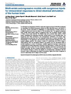
yt = �1yt;1 + � � � + �pyt;p + �t t = 1� :::� n� (28) �t N (0� �2)� where yt is the observation at time t. We present two examples to illustrate our models. The rst example analyses a data set of monthly exchange rates for the Swiss Frank/Index for the period June 1973 to May 1984 (shown in Fig. 3 ) using AR(1) models. The time series are analyzed in di�erenced form, giving 150 observations of monthly 12
exchange rates. The second example estimates AR(1) models for daily exchange rates of the Swiss Frank/US $ in 1987 (shown in Fig. 11). The time series is given in di�erenced form, giving 246 observations of daily exchange rates. We ran the results for the normal distribution shown in Fig. 4 and Fig. 12, the t distribution with priors v = 4, � = 1, and � = 1000 shown in Fig. 5 and Fig. 13, and the hyperbolic distribution with priors � = 1, and
� = 1000 shown in Fig. 6 and Fig. 14. The means and standard errors of the parameters are shown in Table 2 for the SFr./Index, and in Table 3 for the SFr./US$. Particularly the histograms of the SFr./Index and SFr./US$ are compared with normal, hyperbolic distribution in Fig. 17 and 18 respectively. For the model selection, we have calculated the pseudo-Bayes factors based on the conditional predictive ordinates (CPO) for all time points (t = 1� :::� T ) AR(1) models are shown in Table 1.1 for the SFr./Index and SFr./US$ and in Table 1.2 we compare the pseudo-Bayes factors in (26) for up to order p = 4 and the t and hyp-ARMA(1,1) model. For all these models the hyperbolic AR model turns out to give the best t. In Table 1.3 we have calculated the pseudo-marginal likelihood (27) for selection of the order of the order of ARMA(p,q) process. The ARMA(1,1) model is selected (from the range 1 � p � 4 and 1 � q � 4) better than the t4-ARMA(1,1) model. The CPO plots for SFr./Index normal, t4 and hyperbolic distribution are shown in Fig. 7, 8, 9, and 10. From these gures it is seen that the medians of the CPO plots are very similar for t innovations and hyperbolic models. The medians of the CPO plots for t innovations and hyperbolic distribution are larger than those for normal distribution. The CPO plots of the SFr./US$ are shown in Fig. 15. Again we see from these gures that the medians of the CPO plots are very similar. The medians of the CPO plots for the hyperbolic are larger than those for normal distribution and t innovations. The median of the CPO plots for hyperbolic AR(1) model is larger than those for the AR(2), AR(3) and AR(4) model.
6 Conclusions IThis paper has developed a MCMC technique to estimate ARMA(p,q) models with tv and hyperbolic distributed innovations. We have derived the 13
complete conditional distributions for simulation of the posterior distribution by introducing an mixture model for the scale parameters of the normal distribution. The convergence of the Gibbs sampler for monthly and daily exchange rate data (SFr./US$ from June 1973 until May 1984) was achieved very quickly. For the model choice we have used conditional predictive ordinates (CPO's) and the pseudo-marginal likelihood (PsML) criterion which was suggested by Gelfand and Dey (1994). Additionally, pseudo-Bayes factors can be computed to choose between competing models. From the analysis we see that the hyp-ARMA(1,1) model dominates the normal or t distributed ARMA models. This shows that the exchange rate data favor a leptokurtic distributed time series model, like the hyp-ARMA(p,q) model. The leptokurtic e�ect can be seen also for the predictive distribution. Using the MCMC approach we can obtain the small sample distribution for all the parameters and using the pseudo-marginal likelihood criterion we can do test and model choices. Further studies will show how the hyp-ARMA model can be extended to GARCH models and multivariate models (VAR).
A Appendix: The GIG distribution A distribution which is not widely known in econometrics is the generalized inverse Gaussian distribution GIG(x) which has the density =2 ;1 f (xj�� �� ) = (�= )q x exp�; 12 ( x;1 + �x)] for x � 0 2K ( ( �))
(29)
where K (�) (see Appendix B) is the modi ed Bessel function of the third kind with index �. The domain of variation of the three parameter GIG distribution is
> 0� � � 0 if � < 0�
> 0� � > 0 if � = 0�
� 0� � > 0 if � > 0:
Lemma A1: Properties of the GIG distribution. Let GIG(�,�,�) and Ga(�) denote GIG and gamma distribution, respectively, 14
and let all random variables be independent. Then we have the following distributional equivalences (see Devroye 1986, p. 479): ( a) ( b) (c) (d)
GIG(�� �� ) = 1c GIG(�� �c � c) for all c > 0:
s
q q
GIG(�� �� ) = � GIG(�� � � � )� GIG(�� �� �) = GIG(;�� �� �) + �2 Ga(�)� GIG(�� �� ) = GIG(;1�� � �) :
Furthermore the mode is given by
1: Mode = q ;11 2 ; � ; � ( ) +1
Special cases of the GIG distribution are the gamma distribution ( = 0), the reciprocal gamma distribution (� = 0), the inverse Gaussian distribution (� = ; 12 ), and the inverse Gaussian or random walk distribution (� = 12 ). The general hyperbolic density function is a four-parametric density given by p�� q q expf; 21 �(�+� ) �2 + (x ; �)2+(�;� )(x;�)]g� f (xj�� �� �� �) = �(� + � )K1 (� (�� ) (30) where K1(�) is the modi ed Bessel function of third kind (see Appendix B). If X is general hyperbolic distributed with the parameters �, �, �, and � , i.e. X Hyp(�� �� �� � ) then the rst two moments are E (X ) = � + �(2�p;��� ) � V ar(X ) = �: 15
Consider the symmetric centered case of the 4-parametric hyperbolic distribution Hyp(�� �� �� � ) that is, � = 0, � = �� and
q
� = (1 + � �� );1=2: Then the hyperbolic density (8) can be written as a 2-parametric hyperbolic density
p
;2 2 2 f (xj�� � ) = 2�K (�1;2 ; 1) expf; (� ; 1)� � + x g� 1 2
(31)
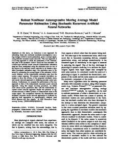
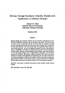
where j � j< 1 and 0 < �2 < 1. In Fig. 1, the standard normal density function is compared with the hyperbolic density function (30) for the parameter values with � = 0:5, � = 0:6 and � = 0:7 (for � = 1). In Fig. 2, the hyperbolic density function in (31) for � = 0:5 and � = 1:0 (� = 0:0, � = 1:0, � = 3:0 and � = 3:0) is compared with the hyperbolic density function (30) with the di�erent parameter values �, �, � and � .
B Appendix: Bessel function of the third kind The Bessel function of the third kind with index 1 is given by 1 X 2)2k+1 ��(k) + �(k + 1)] K1(x) = �ln( x2 ) + � ]I1(x) + x1 ; 12 k(x= !(k + 1)! k =0 with
3 5 I1(x) = x2 + 22x� 4 + 22 �x42 � 6 + � � �� �(k) = 1 + 21 + � � � + k1 � �(0) = 0� and � = 0:5772156 is the Euler constant. The general Bessel function with index � is de ned by Z1 1 cosh(�u)e;xcosh(u) du: K (x) = 2 ;1
16
When (� = 12 ) or (� = ; 12 ), we nd
s
s
2 sin x� and K 1 (x) = 2 cos x� K 21 (x) = �x ;2 �x
v u t ��) = u
q
K; 12 (
2 cos q��: �(�� ) 21
C Appendix: Mixture distributions C.1
t
innovations as a normal-gamma mixture
Lemma C1: The t distribution is a scale mixture of a normal and a gamma ( 2)-distribution. Consider a centered normal distribution
�j�2 N (0� �2)� and the precision �;2 is 2-distributed 1 2� v 2 v then the standardized variable �= is t distributed with v degrees of freedom: � j� t : v Proof: Since the 2 distribution is a special case of the gamma distribution we have 2 �0 = v �2 Ga(v=2� 1=2)� (� )v=2;1expf; 0 g �(�0) = 0 ;(v=2)2v=2 2 � 2)v=2expf; v�2 ( v 2g 2 2 �(� j ) = ;(v=2)2v=2 (�2)v=2 2+1 �
�;2j 2
17
and integrating out �2 yields
�(�j ) =
Z
�(�j�2)�(�2j 2)d�2 Z 1 2 (v 2)v=2 expf; v�2 g � 2 d�2 = 2 p 2 expf; 2�2 g ;(v=2)2v=2 (�2)v=2 2+1 2�� v +1 �2 ; +1 ;( )(1 + ) 2 2 v� 2 p = 2;(v=2) �v : Consider the density function of the standardized variable �0 = �= , 2
2
v
�2 ; +1 ;( v+1 )(1 + v� ) 2 � 0 2 �( ) = ;(v=2)p2�v �20 ; +1 v +1 ;( ) 2 � 2 )(1 +p v� 2 = ;(v=2) �v then this is clearly a t distribution with v degrees of freedom � j�2 t : v v
v
C.2 Hyperbolic distribution
Lemma C2: The hyperbolic distribution can be represented as a mixture
of the normal and the general inverse Gaussian (GIG) distribution. We consider the symmetric hyperbolic distribution (31), so we have to deal only with the location parameter � and the scale parameter �2. Consider the central normal distribution
�j�2 N (0� �2)� and assume a GIG distribution for �2 (�2j� = 1� 2� �) �;2 ; 1 GIG(� = 1� 1� �;2 ; 1) then the mixture distribution is hyperbolic
�j � � Hyp( � �): 18
Proof: Because the normal density is 2 f (�j�2) = p1 expf; 2��2 g � 2� and the hyper-parameter �2 has the density
expf; 21 � (�;�2;1)2 + � ]g �;2 ; 1 �(� j � �) = 2 K (�;2 ; 1) � 2 1 The 2-parameter hyperbolic distribution is obtained by integrating out �2 from the joint density 2
Z
2
p
� ;2 ;1 2 + �2g : exp f; � f ( � j � ) � ( � j � � ) d� = 2 2 K1(�;2 ; 1)
2
2
2
2
References �1] Bagpunar, J. (1988). Principles of random variate generation, Oxford Science Publications. �2] Barndor�-Nielsen, O. E. (1977). Exponentially decreasing distributions for the logarithm of particle size, Proceedings of the Royal London A, 353, 401-419. �3] Barndor�-Nielsen, O. E. (1997). Normal Inverse Gaussian Distributions and Stochastic Volatility Modelling, Scand. J. of Statistics 24, 1-14. �4] Barndor�-Nielsen, O. E., Jensen, J. I. and Sorensen, M. (1989). Wind Shear and Hyperbolic Distributions, Boundary-Layer Meteorology 49. 417-434. �5] Berger, J. O., Pericchi, C. R. (1996). The intrinsic Bayes factor for model selection and prediction, JASA 91, 109-122. �6] Box, G. E. P. and Jenkins, G. M. (1976). Time Series Analysis: Forecasting and Control, Holden Day, San Fransisco. 19
�7] Chib, S. and Greenberg, E. (1994). Bayesian inference in regression models with ARMA(p,q) errors, Journal of Econometrics, 64, 183-206. �8] Devroye, L. (1986). Non-uniform Random Variate Generations, Springer-Verlag, New York. �9] Eberlein, E. and Keller, U. (1995). Hyperbolic Distributions in Finance, Bernoulli 1, 281-299. �10] Engle, R.F. (1982). Autoregressive conditional heteroscedasticity with estimates of the variance of U.K. in$ation, Econometrics 50, 987-1008. �11] Fama, E. (1965). The behavior of stock market prices, J. of Business 38, 34-105. �12] Gelfand, A. E. and Dey, D.K. (1994). Bayesian model choice asymptotics and exact calculations, JRSSB, 56, 501-514. �13] Gelfand, A. E. and Smith, A. F. M. (1990). Sampling based approaches to calculating marginal densities, Journal of the American Statistical Association, 85:398-409. �14] Gelman, A. and Rubin, D.B. (1992). Inference from iterative simulation using multiple sequences, (with discussion), Statistical Science, 7(4), 457-511 �15] Geman, S. and Geman, D. (1984). Stochastic relaxation, Gibbs distribution and the Bayesian restoration of images, IEEE Transactions on Pattern Analysis and Machine Intelligence, 6:721-741. �16] Geisser, S. (1980). Discussion of the paper by G.E.P. Box, JRSSA, 143, 416-417. �17] Geyer, C. (1991). Markov chain Monte Carlo maximum Likelihood, Computing Science and Statistics, 156-163. �18] Hastings, W.K. (1970). Monte Carlo sampling methods using Markov chains and their applications, biometrica, 57, 97-109. �19] Mandelbrot, B. B. (1963). The variation of certain speculative prices, J. of Business 36, 394-410. 20
�20] Metropolis, N. Rosenbluth, A.W. Rosenbluth, M.N. Teller, A.H. and Teller, E. (1953). Equations of state calculations by fast computing machines, �21] M!uller, P. (1994). Metropolis posterior integration schemes, Stat. Computing., forthcoming. �22] Norman, L. J. and Samuel, K. (1970). Sampling Techniques, Wiley series in probability and mathematical statistics, 149. �23] Pai, J. and Ravishanker, (1996). ,Bayesian Modelling of ARFIMA Processes by MCMC Methods, J of Forecasting 15, 63-82. �24] Tanner, M. and Wang, W. (1987). The calculation of posterior distributions by data augmentation, (with discussion), Journal of the American Statistical Association, 82:528-550. �25] Tierney (1994). Markov chains for exploring posterior distributions, (with discussion), Ann. Statistics 22, 1701-1786.
21
SFr./Index SFr./US$ Hyp=N or 717.75232 1.07906 Hyp=t(4) 69.84747 1.47597 t(4)=N or 10.27599 0.731085 Table 1.1: Pseudo-Bayes factors (PsBF) of AR(1) models for SFr./Index and SFr./US$ AR(2) AR(3) AR(4) ARMA(1,1) Hyp=N or 7767.93 3630.67 8.7701 272.2072 Hyp=t(4) 1123.82 8172.67 7.7890 237.4144 t(4)=N or 6.91207 0.4442 1.1259 1.1465 Table 1.2: Pseudo-Bayes factors (PsBF) of AR(2), AR(3), AR(4) and ARMA(1,1) models for SFr./US$ p 1 1 2 3 4 1 1 1 2 3 4 p 1
q hyp-ARMA 0 -299.5067 1 -296.2734** 1 -296.3969 1 -299.3074 1 -300.6974 2 -298.1801 3 -299.4493 4 -299.1183 2 -303.2661 3 -301.3219 4 -307.2369 q t5-ARMA 1 -296.9873
t1-ARMA -307.1074 -302.2248* -306.1095 -307.5711 -305.7271 -306.5814 -307.4177 -306.6823 -305.5267 -304.6712 -306.0763 t6-ARMA -296.9852
t2-ARMA -299.0349 -296.9265* -298.4662 -298.6821 -299.5723 -300.3152 -301.2512 -299.6388 -300.8965 -301.6731 -302.7483 t7-ARMA -296.7322
t3-ARMA -299.2931 -297.3909* -298.5534 -298.6272 -299.9052 -300.6721 -301.7273 -300.5126 -301.3012 -302.6388 -303.7481 t8-ARMA -296.7311
t4-ARMA -308.0917 -297.1681* -297.7808 -300.7323 -301.6563 -297.3510 -298.9292 -298.0368 -319.9409 -317.6383 -326.7722 t9-ARMA -297.1494
Table 1.3: The log marginal likelihood (PsML) for SFr./US$
22
Nor t(4) Hyp Model Mean St. error Mean St. error Mean St. error 0.40683 8.81e-04 0.40953 3.65e-04 0.40428 4.94e-04 AR(1) 1 � 3.18054 2.55e-03 3.08906 2.41e-03 3.18421 2.56e-03 � 1.12084 3.81e-03 6.28449 3.72e-03 � 0.57964 6.86e-04 0.48602 1.00e-03 0.48398 4.15e-04 0.48555 5.32e-04 AR(2) 1 -0.19215 5.28e-04 2 -0.18871 1.01e-03 -0.18908 4.05e-04 � 3.16668 2.60e-03 3.00549 2.32e-03 3.07802 2.55e-03 � 1.12561 3.88e-03 6.31098 3.96e-03 � 0.58340 7.18e-04 0.48580 1.02e-03 0.48497 4.17e-04 0.48661 5.38e-04 AR(3) 1 -0.19884 5.88e-04 2 -0.19785 1.18e-03 -0.19827 4.28e-04 0.01776 1.04e-03 -0.01679 3.94e-03 -0.01866 5.55e-04 3 � 3.26154 2.99e-03 3.00013 2.21e-03 3.08530 2.40e-03 � 1.08220 3.73e-03 6.11120 3.54e-03 � 0.58173 6.95e-04 0.48046 1.07e-03 0.48809 3.93e-04 0.49098 5.46e-04 AR(4) 1 -0.19412 5.97e-04 2 -0.17889 1.14e-03 -0.19393 4.34e-04 0.00108 4.31e-04 -0.00103 5.89e-04 3 -0.01167 1.21e-03 0.03616 1.10e-03 0.03483 3.80e-04 0.03726 5.42e-04 4 � 3.35717 2.91e-03 3.01753 2.25e-03 3.08315 2.43e-03 � 1.08712 3.79e-03 6.49160 3.78e-03 � 0.57391 7.02e-04 Table 2: The means and standard errors of the parameters , � , � and � for SFr./Index
23
Nor t(4) Hyp Model Mean St. error Mean St. error Mean St. error 0.00807 2.95e-06 0.00809 2.00e-06 0.01001 2.68e-04 AR(1) 1 � 0.00013 4.80e-08 0.00012 4.52e-08 0.00012 4.42e-08 � 0.00006 2.60e-08 0.00028 1.05e-06 � 0.57587 4.41e-04 0.00862 3.03e-06 0.00864 1.90e-06 0.00942 2.65e-04 AR(2) 1 -0.06319 2.62e-04 2 -0.06336 2.97e-06 -0.06335 2.25e-06 � 0.00013 4.58e-08 0.00012 4.17e-08 0.00012 4.48e-08 � 0.00006 2.48e-07 0.00024 9.07e-07 � 0.58712 4.29e-04 0.00296 2.86e-06 0.00292 1.97e-06 0.00087 2.68e-04 AR(3) 1 -0.06292 2.64e-04 2 -0.06266 3.05e-06 -0.06270 2.22e-06 0.09176 3.07e-06 -0.09176 2.00e-06 -0.09280 2.63e-04 3 � 0.00013 4.60e-08 0.00012 4.34e-08 0.00012 4.70e-08 � 0.00006 2.56e-07 0.00022 8.33e-07 � 0.59721 4.37e-04 0.00404 2.98e-06 0.00404 1.95e-06 0.00727 2.65e-04 AR(4) 1 -0.05793 2.62e-04 2 -0.17889 3.13e-06 -0.19393 2.27e-06 -0.09486 2.66e-04 3 -0.09177 3.14e-06 -0.09177 2.28e-06 0.01238 3.10e-06 0.01237 2.05e-06 0.01203 2.56e-04 4 � 0.00013 4.65e-08 0.00012 4.33e-08 0.00012 4.61e-08 � 0.00006 2.52e-07 0.00025 8.63e-07 � 0.57911 4.32e-04 Table 3: The means standard errors of the parameters , � , � and � for SFr./US$
24
0.8 0.6
Hyp(0.5, 1)
Hyp(0.6, 1) 0.4
Norm(0, 1) t(4)
0.0
0.2
Hyp(0.7, 1)
-3
-2
-1
0 data
1
2
Figure 1: The standard normal density N (0� 1) compared with the hyperbolic density Hyp(�� �) and t(4). 25
3
0.8 0.6 0.4 0.2 0.0
0.8 0.6 0.4 0.2 0.0
hyp(0,1,4,3) ••••• •• •• ••• ••••• •• •••• hyp(0,1,2,3) ••• ••• ••• ••• ••• ••• ••• •• ••• •• ••• • • ••••• • • • • ••••••••••••••• • • • • • • •••••••••••• ••••••••••••••••••••• -3 -2 -1 0 1 2 3
••••••• ••• ••••• •• •••• ••• ••• • ••• ••• ••• •• ••• •• ••• •• ••• • • •••• • • • ••••••••• • • • • • • • • •••••••••••••••••••• ••••••••••••••••••••• -3 -2 -1 0 1 2 3
-0.03
-0.01
0.01
SFr./US$
0
50
100
150
-6 -4 -2 0
2
4
6
SFr./Index
0
50
100
150
Figure 3: Monthly exchange rate for Swiss Franc/Index from Jan. 1973 to May 1984 27
0.8 0.6 0.0
0.2
phi 0.4
200
400 600 SFr/Index
800 1000
0
50 100150 200 250
0
0.0
0.2
0.4 phi
0.6
0.8
0.25 0.20 0.15 0.10 0.05 0.0
(1,0)(2,0)(3,0)(4,0)(1,1)(2,1)(3,1)(4,1)(1,2)(2,2)(3,2)(4,2)(1,3)(2.3)(3,3)(4,3)(1,4)(2,4)(3,4)(4,4
Figure 7: CPO plots of monthly rates(SFr./Index) for normal AR(p,q) models 31
0.25 0.20 0.15 0.10 0.05 0.0
(1,0)(2,0)(3,0)(4,0)(1,1)(2,1)(3,1)(4,1)(1,2)(2,2)(3,2)(4,2)(1,3)(2.3)(3,3)(4,3)(1,4)(2,4)(3,4)(4,4
Figure 8: CPO plots of monthly rates(SFr./Index) for mixture normal-t innovations AR(p,q) models 32
0.25 0.20 0.15 0.10 0.05 0.0
(1,0)(2,0)(3,0)(4,0)(1,1)(2,1)(3,1)(4,1)(1,2)(2,2)(3,2)(4,2)(1,3)(2.3)(3,3)(4,3)(1,4)(2,4)(3,4)(4,4
Figure 9: CPO plots of monthly rates(SFr./Index) for hyperbolic AR(p) models 33
(2,0) (4,0) (2,1) (4,1)
34 (2,2) (4,2) (2,3) (4,3) 0.05
0.10
0.10
0.15
0.15
0.15
0.20
0.20
0.20
0.20
0.25
0.25
0.25
0.25
0.25
(3,3)
0.0
0.05
0.10
0.15
0.20
0.25
0.25
(1,3)
0.0
0.05
0.10
0.15
0.20
0.20
0.25
0.25
0.25
(3,2)
0.0
0.05
0.10
0.15
0.20
0.20
0.20
(1,2)
0.0
0.05
0.10
0.15
0.15
0.15
0.15
(3,1)
0.0
0.05
0.10
0.10
0.10
0.10
(1,1)
0.0
0.05
0.05
0.05
0.05
(3,0)
0.0
0.0
0.0
0.0
(1,0) (1,4)
(2,4)
Figure 10: CPO plots of monthly rates(SFr./Index) for normal, t4-AR(p) and hyperbolic AR(p) models (3,4)
(4,4)
0.0
0.0
0.0
0.0
0.0
0.0
0.0
0.0
0.0
0.0
0.05
0.05
0.05
0.05
0.05
0.05
0.05
0.05
0.05
0.05
0.10
0.10
0.10
0.10
0.10
0.10
0.10
0.10
0.10
0.10
0.15
0.15
0.15
0.15
0.15
0.15
0.15
0.15
0.15
0.15
0.20
0.20
0.20
0.20
0.20
0.20
0.20
0.20
0.20
0.20
0.25
0.25
0.25
0.25
0.25
0.25
0.25
0.25
0.25
0.25
-0.02
data 0.0
0.02
0.04
SFr.-US$ in 1987
0
50
100
150 Index
Figure 11: Daily exchange rate for SFr./US$ in 1987 35
200
250
delta 0.00014
0.010 0.006
0.00010
phi 0.008
200
400 600 Index
800 1000
0
200
400 600 Index
800 1000
0
0
100
200
300
50 100 150 200 250
0
0.006 0.007 0.008 0.009 0.010 phi
0.000080.000100.000120.000140.000160.00018 delta
Figure 12: AR(1) model of daily exchange rates(SFr./US$) for N (0� �2) 36
0.00016
0.0004 0.0
0.00010
0.0001
0.00012
delta
sigma 0.0002
0.00014
0.0003
0.010 phi 0.008 0.006 0.004
0
200
400
600
800
1000
0
200
400
600
800
1000
0
200
400
600
800
1000
Index
0.004
0.006
0.008 phi
0.010
0.012
100 0
0
0
100
200
200
300
200
400
400
500
300
Index
600
Index
0.0
0.0001 0.0002 0.0003 0.0004 sigma
0.00010
0.00012 0.00014 delta
Figure 13: The Gibbs output of the t4-AR(1) model of daily exchange rates(SFr./US$) 37
0.00016
400 600 Index
800 1000
200
400 600 Index
800 1000
400
0
0
200
400 600 Index
800 1000
-0.2
-0.1
0.0 phi
0.1
0.2
0.4
0.5
0.6 ksi
0.7
0.8
0
0
0
0
50
100
50
50
100
200
150
100
100
300
250 200
0.00010
0.0
200
150
0
150
800 1000
delta 0.00012
sigma 0.0010 0.0005
ksi 0.6 0.5 0.4
400 600 Index
0.00014
0.0020 0.0015
0.8 0.7
0.2 0.1 phi 0.0 -0.1 -0.2
200
300
0
0.0
0.0005 0.0010 0.0015 0.0020 sigma
0.00010 0.00012 0.00014 0.00016 delta
Figure 14: The Gibbs output of the hyp-AR(1) model of daily exchange rates(SFr./US$) 38
40 30 20 10 0
0
0
10
10
20
20
30
30
40
40
40 30 20 10 0
(1,0)
(2,0)
(3,0)
0.20
0.25
Figure 15: CPO plots of daily exchange rates(SFr./US$) for normal, t4 and hyperbolic AR(p) models for p = 1� : : : � 4
(4,0)
0.05
0.10
0.15
Nor(0,3.18054)
SFr./Index
0.0
Hyp(6.28449,0.57964)
-10
-5
0
5
Figure 6: The histogram of SFr./Index compared with Nor(0,�) and Hyp( ,�) 39
10
40 30 20 10 0
-0.04
-0.02
0.0
0.02
0.04