AverageExplorer: Interactive Exploration and Alignment f Visual Data ...

AverageExplorer: Interactive Exploration and Alignment of Visual Data Collections Jun-Yan Zhu

Yong Jae Lee

Alexei A. Efros

University of California, Berkeley

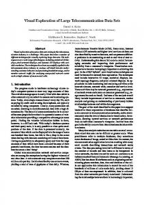
c Jason Salavon (a) are a creative way to visualize image data. However, attempts to Figure 1: Average images, such as ‘Kids with Santa’ replicate this technique with data automatically scraped from the Internet (b) does not lead to good results (c,d). In this work, we propose an interactive framework for discovering visually informative modes in the data and providing visual correspondences within each mode (e).

Abstract This paper proposes an interactive framework that allows a user to rapidly explore and visualize a large image collection using the medium of average images. Average images have been gaining popularity as means of artistic expression and data visualization, but the creation of compelling examples is a surprisingly laborious and manual process. Our interactive, real-time system provides a way to summarize large amounts of visual data by weighted average(s) of an image collection, with the weights reflecting user-indicated importance. The aim is to capture not just the mean of the distribution, but a set of modes discovered via interactive exploration. We pose

this exploration in terms of a user interactively “editing” the average image using various types of strokes, brushes and warps, similar to a normal image editor, with each user interaction providing a new constraint to update the average. New weighted averages can be spawned and edited either individually or jointly. Together, these tools allow the user to simultaneously perform two fundamental operations on visual data: user-guided clustering and user-guided alignment, within the same framework. We show that our system is useful for various computer vision and graphics applications. CR Categories: I.3.8 [Computer Graphics]: Applications—; Keywords: big visual data, average image, data exploration Links:

1

DL

PDF

Introduction

The world is drowning in a data deluge [The Economist, Feb 25th 2010], and much of that data is visual. An estimated 3.5 trillion photographs have been taken since the invention of photography, of which 10% within the past 12 months. Facebook alone reports 6 billion photo uploads per month; YouTube sees 72 hours of video

uploaded every minute. Additionally, there is the data that hasn’t made it onto the Internet (yet), such as the 24/7 video feeds from millions of surveillance cameras in convenience stores and ATMs. In fact, there is so much visual data out there already that much of it might never be seen by a human being! But unlike other types of “Big Data”, such as text or consumer records, much of the visual content cannot be easily indexed, searched or hyperlinked, making it Internet’s “digital dark matter” [Perona 2010].

average images [Torralba 2001] where a dataset is first centered (aligned) on a particular object (e.g. a face, a spoon, etc) before the average is computed. Torralba’s beautiful averages [Torralba 2001] contrast a sharper focal point with an eerie, dream-like background. Unfortunately, to achieve this effect requires that the object in focus be carefully hand-labeled in all images in the dataset before computing the average, making this approach completely impractical for large-scale data.

How can we explore this vast visual space, to see what’s out there? One way is to anchor off the image meta-data (keywords, surrounding text, GPS, etc) as a proxy for indexing visual content. For example, typing “wedding kiss” into G OOGLE I MAGE S EARCH will return pages upon pages of photos that have somehow been associated with the words “wedding” and “kiss”, most of them actually depicting formal kissing of various sorts (Figure 6a). While this semantic focusing vastly narrows down the data (from {all photos} down to {all wedding kiss photos}), the resulting set is still far too vast to take in by mere visual inspection. How can we capture the visual gestalt of this data, its Platonic ideal?

In this paper, we propose an interactive framework that allows a user to rapidly explore and visualize a large image collection using average images. The idea is to summarize the visual data by weighted averages of an image collection, with the weights reflecting user-indicated image and feature importance. The aim is to capture not just the mean of the distribution, but a set of modes and projections (Figure 1e top), discovered via interactive exploration. The user interactively “edits” the average image using various types of brushes and warps, similar to a normal image editor, with each user interaction providing a new constraint to update the average. The user can also spawn and edit new weighted averages either individually or jointly, in which case an image that is weighted highly in one average will automatically be down-weighted in the others.

The main inspiration and a departure point for this paper is the recent surge in the use of data analytics and visualization techniques in contemporary art [Vi´egas and Wattenberg 2007]. In particular, the simple technique of image averaging has been used extensively, and to great effect, by several well-known contemporary visual artists, such as Krzysztof Pruszkowski [1986], Jason Salavon [2004], James Campbell [2002], and Idris Khan [2005]. An average image of a set of photographs is obtained by simply computing the average color at each (x, y) pixel position independently across the set. This has the effect of capturing the overall similarities within the set while blurring out the individual differences1 . For example, Figure 1a shows a piece by Salavon titled ‘Kids with Santa’, from his 100 Special Moments series [2004], which is an average computed over a hundred photos the artist manually picked from the Internet. Notice how, although the average is quite blurred, one can definitely decipher a figure dressed as Santa Claus, with another figure sitting on his knee – the individuality and uniqueness of each “special moment” usurped to tell a universal story. Alas, we discovered that trying to replicate Salavon’s averages automatically turns out to be quite difficult, e.g. simply downloading the top hundred images using a Google query “kids with Santa” (Figure 1b) and averaging them does not work well (Figure 1c). This is because the data is too varied (e.g. there are close-ups vs. long-range views, Santa could be in vastly different poses, or be missing altogether), and even images that depict the same type of scene (e.g. sitting Santa with kid on left knee) are not spatially aligned resulting in an extremely blurry average. Trying to reduce the data variability by first clustering the images using popular techniques, gives a slight improvement (Figure 1d), but nowhere close to Salavon’s hand-picked average. Of course, it is an artist’s role to “actively guide analytical reasoning and encourage a contextualized reading of their subject matter” [Vi´egas and Wattenberg 2007], but the only active guidance available in image averaging is the choice of which images to include – a blunt and inefficient instrument. What if we wanted to bring into focus different parts of the average image, such as Santa’s face, or that of the kid? Antonio Torralba (a computer scientist who is also an accomplished artist) has been working on centered 1 In fact, this technique is almost as old photography itself, going back to Sir Francis Galton who, “having obtained photographs of several persons alike in most respects, but differing in minor detail”, created “composite portraits” by “throwing faint images of the several portraits, in succession, upon the same sensitised photographic plate” as way of “extracting typical characteristics from them” [Galton 1878].

Alternatively, one can view the proposed framework as a new way to perform two fundamental operations on visual data: user-guided clustering and user-guided alignment. Automatic (i.e. unsupervised) image clustering and image alignment are, of course, two key problems in computer vision, both largely unsolved. By bringing the user into the loop, we demonstrate how to address these two problems jointly, within the same framework. And while our main driving application is in Big Visual Data exploration and improved artistic expression, we also demonstrate our framework to be of value in various other computer vision and graphics tasks.

2

Prior Work

Our work builds on ideas from a number of different areas: Image stacks: Given a stack of (typically) registered images of the same subject matter, methods such as Photomontage [Agarwala et al. 2004] offer various multi-image pixel operations on the stack, resulting in a combined “best” image. Our approach shares the idea of operating on an image stack, except our stack is 1) made up of semantically, but not necessarily visually similar data, 2) not typically well aligned, and 3) far too large for any manual per-image user guidance. Also related, a computer vision technique called congealing [Learned-Miller 2006; Huang et al. 2007a] jointly aligns a stack of images of the same object category by iteratively bringing each image into closer alignment with the average. A recent extension [Mattar et al. 2012] can even jointly align and cluster simple digit images. The congealing pipeline is fully automatic and while it works quite well for simple, unimodal categories (e.g. digits) and small mis-alignments, due to its iterative nature, it often falls into local minima on more complex image data. Image clustering and data mining: A standard way to model and visualize multi-modal data is by clustering. However, clustering is a highly under-constrained problem [Balcan and Blum 2008], so most clustering algorithms, such as k-means, spectral clustering [Shi and Malik 2000], make strong distributional assumptions about the data and/or the distance metric, which often produce results that do not correspond to what is anticipated by the user. The present work can be thought of as a type of interactive clustering [Balcan and Blum 2008] where the user can refine clustering results via interactive feedback. Other efforts aim to mine visual collections by finding a small number of important or “iconic” images [Simon et al. 2007; Berg and Berg 2009] or visual elements [Doersch et al. 2012]. We differ in that our aim is to cap-

ture the gestalt of the data, not sample from it (although our system provides the latter as well). Unsupervised sub-category discovery approaches [Divvala et al. 2012; Hoai and Zisserman 2013] use discriminative clustering to find multiple modes for a given visual category. However, these methods do not provide local image alignment, resulting in poor clusters (see Sec. 4). Data-assisted content editing and content creation: There has been recent interest in using large amounts of online visual data as content for computer graphics. For example, Hays and Efros [2007] use millions of Flickr images as data for filling holes in a given scene, whereas Sketch2Photo [Chen et al. 2009] allows a user to generate new visual content by employing sketch and text queries to find and compose together content from existing photographs. There are also methods that use large amounts of data to provide artistic guidance to the user as part of the content creation process. Most related to our work is ShadowDraw [Lee et al. 2011], which helps users draw better by providing real-time average “shadow” suggestions of what to draw next by matching what has already been drawn against a large database of existing imagery. Our sketching brush tool is very much inspired by ShadowDraw, but whereas ShadowDraw is fundamentally a reactive, bottom-up process – first asking the user to draw something and only then providing suggestions, our system aims to be top-down – first giving the user a sense of what is in the data, and only then asking him to refine it. More importantly, the target goals are fundamentally different: while ShadowDraw aims to help the user in drawing, our AverageExplorer aims to help the user in exploring and aligning large image collections, while also facilitating a number of other applications (Sec. 4). Inspired by successful content-based image retrieval systems like Fast Multiresolution Image Querying [Jacobs et al. 1995] and BlobWorld [Carson et al. 2002], our system also takes paint strokes and user-specified regions as input (Sec. 3.3). Exploratory data visualization: There is a large body of work on exploring and mining Big Data in a visual way (see [de Oliveira and Levkowitz 2003] for a survey), but the vast majority is on visualizing non-visual data, which is rather different from the problem we are trying to address. Several works show beautiful ways of visualizing a specific type of visual data, such as photos of the same location [Snavely et al. 2006], or of the same person [KemelmacherShlizerman et al. 2011]. Of the few attempts to visualize generic, large-scale visual data, the most related is the “Visual Dictionary of Tiny Images” [Torralba et al. 2008], that aims to provide a visual summary of 80 million images using an atlas of 53464 tiny average image tiles, each corresponding to one English noun. While the online demo is fun to explore, semantic concepts (words) often do not correspond to coherent visual concepts, making many of the average images noisy and uninformative. In this work, we only use semantics (e.g. keyword tags) as an initialization, and then let the user interactively discover visual concepts hidden in the data.

3

Approach

AverageExplorer is a real-time interactive system that allows the user to easily explore and navigate a large image collection through the manipulation of average image(s). The input is a (potentially very large) collection of images, typically representing the same semantic concept (“cats”, “shoes”, “Paris”, etc.) but with wide variation in appearance, e.g. Internet images retrieved using a search engine. The output is a set of average images that depict different modes in the data, as well as feature correspondences between images within each mode. The user is provided with a set of brush tools to iteratively “edit” each average image. The objective is to summarize the image collection with weighted average(s) of images, in which the weights reflect the user’s suggested importance. AverageExplorer has five main components: (1) the user interface,

which displays one or more average images that reveal different modes in the data; (2) a method to generate/update an average image, which continuously takes the user’s edits and re-ranks the database images accordingly; (3) a set of brush tools (explorer, coloring, and sketching), which the user applies to the average image to denote what she deems important; (4) cluster spawning, which dynamically creates a new cluster at anytime for simultaneous exploration of multiple average images; and (5) image alignment, which automatically warps each image in the dataset to better align it with the user-specified constraints.

3.1

User interface

The AverageExplorer interface is composed of the current average image, a button for each brush tool, a button to generate a new cluster, and a retrieval display of the top most similar (i.e. highestweighted) images to the current average. The average image and retrieved images are updated in real-time as the user continuously provides edits. When the user makes an edit, it is highlighted on both the average image and in each of the retrieved images. If more than one average image is being edited, the user can switch focus between them by pressing the ‘tab’ key or clicking on the corresponding cluster with the mouse cursor (see video).

3.2

Generating the average image

Given a database of N images {I1 , . . . , IN }, we continuously update its average image in real-time as the user interacts with the system. We create the average image Iavg by computing a weighted average of the database images that reflects the score (i.e. weight) si of each image (for now, we assume that the images are spatially aligned; in Sec. 3.5, we will relax this assumption): PN Iavg =

i=1 P N

si · Ii

i=1

si

.

(1)

We initialize si = 1/N, ∀i so, we start with Iavg being a simple pixel-wise mean of the entire image collection. Once editing begins, the score si for each image Ii is updated to reflect how well that image matches the user’s edits, and is computed cumulatively: si =

PT

t t=1 match(wuser , Ii ),

(2)

t where si is the cumulative score of image i after T edits, wuser represents the user edit at time t, and match(·) returns how similar a t given image Ii is to the user edit wuser . For now, we will define t t match(wuser , Ii ) = wuser · φ(Ii ), i.e. the dot-product between the t user edit wuser and image Ii in some feature space defined by φ(·). t (the exact representation of wuser and φ(·) depends on the type of user edit and will be defined in Sec. 3.3). Intuitively, each user edit tells the system which visual patterns should be present (or emphasized) within the spatial region where the edit has occurred. An image that has similar visual patterns as the user’s edit will produce a high match(·) value, while an image that has dissimilar visual patterns will produce a low match(·) value. Because the image scores are computed cumulatively, we only need to update the score to reflect the latest edit, which allows our system to update the average image very quickly and smoothly from one edit to the next.

To reduce the effect of noisy matches produced when editing has just started (e.g. with a single edit, there can be a few matches that agree extremely well at the local region level, but not at the global image level), we apply the following nonlinear function (also used by [Lee et al. 2011] for a similar purpose) to each image score: s∗i = max(0, si − α · s¯)γ , where s∗i is the updated image score, s¯ is the average of the top K image scores, α = 0.2 + 0.05 ·

Figure 2: We propose a set of brush tools that can be used to edit the average image to interactively explore the data. Each user interaction provides a new constraint to update the average. T , γ = 0.1 · T , and K = 20. As α increases, fewer images will have score greater than 0, and as γ increases, the distribution of those positive scores will become more peaked. The combined effect makes the average image blurry initially and sharper over time (i.e. as T increases).

3.3

Brush tools

AverageExplorer provides three brush tools to navigate the data: coloring, sketching, and explorer. Each tool allows the user to dynamically update the average image. After each edit, the weight of each database image is changed according to how similar it is to all of the user’s edits provided thus far. 3.3.1

Coloring Brush

The coloring brush allows the user to paint on the average image by adding color strokes. The user chooses a color (mouse right button) from either a standard color palette or a “data-driven palette” which contains the most common colors for the region currently under the blush across the dataset. The user can adjust the size of the brush by scrolling the mouse wheel, and color by holding down the left mouse button. This tool is most useful when the user wants to constrain the color of a specific spatial region (e.g. to specify the color of a person’s hair or eyes). We encode the user’s color T stroke at the current iteration T as wuser = Hc , which is a normalized, 5-dimensional (x,y,R,G,B) histogram containing a uniformlysampled 4x4x4 RGB histogram within each 8x8 pixel block of the stroke (see Figure 2d). Each database image Ii is encoded in the same way, φ(Ii ) = Hc,Ii ; a normalized 5-dimensional (x,y,R,G,B) histogram computed in the same spatial region as the user’s color t stroke. match(wuser , Ii ) = Hc · Hc,Ii , a dot-product between the two histograms, encoding the degree of their similarity. As the user paints, the average image is updated dynamically at 30 fps. Figure 2(a) shows an example usage: a user selects the brown color, clicks on the center of the average image and starts painting, giving high weight to the brown images in the dataset, which changes the average image accordingly. 3.3.2

Sketching Brush

The sketching brush allows the user to add line strokes to the average image. The user can choose the size of the brush by scrolling the mouse wheel, and sketch by holding down the left mouse but-

ton. It is most useful for adding fine details (e.g. outlining the shape of the chin or drawing glasses when exploring faces). We T encode the user’s sketch at the current iteration T as wuser = Hg , which is a histogram with spatial and orientation bins encoding the gradients under the stroke region. We use the standard Histogram of Gradients (HOG) representation [Dalal and Triggs 2005] with 8x8 pixel spatial bins (see Figure 2d). Each database image Ii is encoded in the same way, φ(Ii ) = Hg,Ii ; a HOG feature computed in the same spatial region as the user’s line stroke. Thus, t match(wuser , Ii ) = Hg · Hg,Ii , a dot-product between the two histograms, encoding the degree of their similarity. As with color brush, as the user sketches, we dynamically update the average image at 30 fps. Figure 2(b) shows an example usage: the user sketches a diagonal stroke to denote a particular chair leg shape, which gives high weight to the database chair images that have similar shaped legs and updates the average image and the top retrieved images accordingly. 3.3.3

Explorer Brush

The coloring and sketching brushes are useful to emphasize and sharpen the features that are already visible in the average image. However, if the user wants to explore information that may be hidden in the data and not immediately visible through the average, she is essentially limited to guessing the correct stroke. The explorer brush attempts to overcome this limitation; it is thus our most important tool. The main idea is to collect local patches situated in the same spatial position across all database images, and cluster them into a set of visually-informative modes. As part of the explorer tool, the user can pick a single mode, and see the global average computed using only the images that are assigned to (conditioned on) that mode, as illustrated on Figure 3. This give the user a local tool to interactively explore the different components that make up an average image. Specifically, given a mouse cursor position, we find the dominant local modes (groups) in the image stack data for that rough spatial location. To find the modes, we adapt the mid-level discriminative patch discovery approach of [Singh et al. 2012]. It mines mid-level visual patterns that are frequently-occurring but also discriminative (sufficiently different from the rest of the “natural visual world”). We first sample a thousand “seed” patches centered at the mouse cursor position from a random subset of the database images. For each seed, we compute distances to patches from

Initial avg.

Figure 3: Our explorer brush groups local image patches (shown in green bounding boxes) from the same rough spatial position across all database images. Then, for each group, our system averages the full images assigned to the group to create an average image. (roughly) the same spatial position in all remaining database images, and also compute distances to random patches in random images (downloaded from Flickr), which represent the “natural visual world”. For each potential group (seed patch and its k nearest neighbors) we compute the inlier score u, which is the ratio of the database images (inliers) to the Flickr images (outliers) in the k nearest neighbor patches (k = 50 in our experiments). The inlier score measures the uniqueness of the nearest neighbors. A group that includes many Flickr patches will not be unique as it will capture common visual patterns found in the natural world, whereas a group comprised mostly of patches from the database will capture unique visual patterns, and thus be good for matching and alignment (see Figure 3; the top-ranked modes are discriminative and lead to accurate matches). We then rank each group of seed patch pj and nearest neighbors P {d1 , . . . , dN } by: ( N m=1 sm ·z(dm ))·uj , where N is the number of detections (one per image), sm is the score of the image containing patch dm , z(dm ) is the similarity score between pj and dm , and uj is the inlier score. This scoring function will assign high rank to unique groups whose nearest neighbors match well to the seed patch and come from highly weighted images (due to previous edits). This reinforces the gradual change of the average image, since the top suggestions (i.e. highest ranked groups) are likely to come from images that contributed highly to the previous average image (see next paragraph for details on how to choose between different groups). We retain groups that have inlier score u greater than 0.75, and remove near-duplicate groups that have spatial overlap of more than 25% between any 30 patches of their members. This typically results in 10-50 groups that represent the main local modes of the data at that spatial position. The user interaction proceeds as follows: As the mouse hovers over a particular part of the average image, the top-ranked local modes are displayed below the average image, as average local patches (Figure 2c). The user can interactively change the size of the local patches by scrolling the mouse wheel. By default, the main panel displays the average image according to the top-ranked local mode. But the user can explore the average images of the lowerranked modes by pressing the ‘tab’ key, which shifts down to the next mode (Figure 2c). Once the user finds an interesting position on the average image and picks the preferred local mode, she can use this mode as an extra constraint on the average image by pressing the left mouse button. Specifically, we encode the user’s mode T constraint at the current iteration T as wuser = He , which is a histogram of the gradients in the seed patch of the given mode, again using HOG. Each database image Ii is encoded in the same way, φ(Ii ) = He,Ii ; a HOG feature computed in the same spatial ret gion as the selected mode. Thus, match(wuser , Ii ) = He · He,Ii , a dot-product between the user edit’s and database image’s HOGs. This has the effect of constraining the average image to give more

1st edit

2nd edit

3rd edit

Final avg. w/o alignment

Figure 4: We align each database image to produce a sharper average image. Notice how just clustering (without alignment) is insufficient to produce a sharp average (right-most column). weight to the images from that local mode. Real-time speed-up: Unlike the previous tools, the computation required for the explorer tool is too expensive to run in real time due to large amount of patch nearest neighbor searching across the entire dataset, the discriminative patch mining, and the fact that the user wants to explore the space rapidly. To achieve real-time performance, we are forced to pre-compute the matches offline. Specifically, we first sample seed patches on a dense regular grid (4-pixel stride) at multiple scales (32x32, 48x48, 80x80, 128x128 pixel patches) for the entire image collection. We then compute distances (dot-product in HOG space) to all patches within a 2x length (64 to 256 pixels) region surrounding the seed patch in all remaining database images. For each seed, we store the top matching patch per image with match score greater than 0.5, and record both the match score as well as the position and scale of the matched patch. During online processing, for each seed in the current mouse cursor position, our system selects the top-matching patch in each database image to create the average image. Figure 2d shows example usage: given a database of face images initially with uniform weight (top), the user explores different types of mouths (bottom). The user has chosen the second mode, which changes the average image accordingly.

3.4

Interactive Clustering

At any time during data exploration, the user can spawn a new cluster. This is particularly useful when the user wants to explore multiple modes in the data at the same time. For example, when exploring human faces, the user might want to separate, say, people with oval faces from people with rounder faces. To this end, we present a tool for interactive clustering, in which a user’s edit on one average image influences the average images of the other clusters (i.e. modes). The goal is to simultaneously produce sharper average images for all clusters, which means that each cluster should consist of images that are similar to each other and dissimilar to images in other clusters. E.g. if the user edits an average image of a face to be rounder, then the other average images should become oval-shaped. To simultaneously update all clusters with each edit, we compute a cluster-specific weight for each image. The average image for each cluster is created as in Sec. 3.2, but the weight of each image can now be different for each cluster. We normalize the cluster-specific weights in such a way that an image cannot contribute highly to all clusters. Specifically, we initialize a new cluster c by assigning each image with uniform weight si,c = 1/N, ∀i. We then normalize the weights suchP that the total cluster-specific weights of an image sum to one: i.e. j si,j = 1, where j indexes the clusters. In effect, the normalization limits high contribution of an image to one or a

Figure 5: Examples of interactively discovered modes in the data using AverageExplorer. few clusters, which in turn makes each cluster tighter. To give a simple example, if there are two clusters, and the user colors one average image white, then the second average image will become black, since all the highest weighted images for the first cluster will be white, while the highest weighted images for the second cluster will be the opposite (i.e. black).

3.5

Image Alignment

Thus far, we have assumed that the semantic concepts (“cats”, “shoes”, “Paris”, etc) depicted in each database image will be spatially aligned. In practice, this will rarely be the case (even within the same mode), especially when working with Internet images retrieved using a search engine. If the database images are not spatially well aligned, the resulting average will be blurry, which, in turn, will lead to meaningless user edits. AverageExplorer provides a two-step solution to mitigate this problem: robustness to misalignment and image warping. First, we update the matching function so that it is robust to (some) spatial misalignment between the database images using max-pooling [Boureau et al. 2010]: t t match(wuser , Ii ) = max wuser · φp (Ii ), p∈P

(3)

where p indexes over the possible x, y locations in P, and φp (Ii ) is the feature space representation of image Ii computed over the spatial location defined by p. We set P to be the locations that cover up to 64 pixels in both x, y directions surrounding the user’s edit. We then apply non-linear warping to align the database images. For this, we use Moving Least Squares (MLS) [Schaefer et al. 2006], which provides a simple closed-form solution that yields fast deformations for real-time performance. MLS estimates a deformation function that maps a set of source control points to a set of target control points. We use the center of mass of each user edit in the average image as a target control point and the center of mass of the corresponding matching region in the database image as a source control point. We then warp the database image such that its control points (from all T edits thus far) align to the corresponding control points in the average image. The deformation function is applied to every pixel in the database image (see [Schaefer et al. 2006] for more details). Note that the warping does not affect the matching function defined in Eqn. 3; it is used only to align the images more accurately to form a sharper average. We compute the average image with the warped images IiMLS : PN MLS i=1 si · Ii Iavg = . (4) PN i=1 si

Our iterative, user-guided process leads to image stacks that have increasingly better image alignment, producing not only sharper average images (Figure 4), but also surprisingly high-quality local feature correspondences (Figure 1e bottom), which can be useful for rapid data annotation (Sec. 4, “Image annotation”). Finally, after each user edit, we update each database image with its warped version. For non-linear warping, we need to recompute the database image features (HOG, color histograms, and discriminative patches), which is prohibitively expensive. Therefore, we only translate each image according to the mean offset between the source and target control points.

4

Results and Applications

We demonstrate how our system can be used to explore and visualize large image collections, and show several potential applications. Datasets: We experimented with a variety of visual image collections from multiple sources. They are: Labeled Faces in the Wild (LFW) [Huang et al. 2007b], which has 13233 images with 5749 different people; Cat database [Zhang et al. 2008] (10000 images); Query-based collections downloaded from Google Images and Flickr using the following keywords: ‘Church’ (11007 images), ‘Paris’ (7823 images), ‘Butterfly’ (15640 images), ‘Beach’ (8375 images), ‘Wedding kiss’ (16868 images), and ‘Kids with Santa’ (1640 images); YouTube videos: 50 clips of 1 minute summary of the Cobert Report, sampled at 2 fps (5232 frames total); and 362 PASCAL 2007 Horse images. Implementation details: We resize each image to the average size of its dataset. To compute wuser for coloring and sketching we first create a tight bounding box surrounding the user’s stroke or selected region. We then compute the color or HOG histograms over 8x8 spatial bins, and zero-out any cells that do not spatially overlap with the users’ stroke/region. We whiten the HOG descriptors, as described in [Hariharan et al. 2012], which makes dot product similarity computations more visually meaningful. When computing the average image, we ignore any pixels in the warped images that fall outside of the dimensions of the average image. We run our system in real-time on a PC with Intel i7-4770K processor (3.50GHz, 4 cores) and 16GB RAM. For a 10000 image dataset, the pre-computation processing of features and discriminative patch discovery can be done on a 150-core cluster in about 10 hours. Our system is publicly available on our project page. Interactive exploration and alignment: We first show how AverageExplorer can help to uncover meaningful patterns in visual data. We compare against the standard global average of the dataset, as

Figure 6: Interactive exploration and alignment. For each dataset we show (a) example images, (b) global average image, (c) our discovered modes with 4 top retrieved images and automatically marked correspondences (an experienced user spent on average 134 seconds discovering each mode using on average 3.4 user edits), and (d) comparison to [Hoai and Zisserman 2013] cluster averages and representative instances that have the highest confidence scores (i.e., most discriminative). Comparisons to other techniques are in the supp. material. Notice how our averages are sharper and more semantically meaningful, while our retrieved images offer much better correspondence. To visualize the correspondences, we display color strokes for coloring tool (e.g. yellow strokes on the forehead), black strokes for sketching tool (e.g. sketch of glasses), and green bounding boxes for explorer tool.

(a) [Divvala et al. 2012] modes

(b) Our discovered modes

Figure 7: We compare the averages generated by the visual subcategory learning approach of [Divvala et al. 2012] (a) to our averages (b) using the PASCAL 2007 horse dataset. See text for more details.

Random Accuracy (%) Manual Accuracy (%) Ours Accuracy (%) Manual Time (minutes) Ours Time (minutes)

M =3 55.3 66.0 67.4 24 6

M =6 64.9 65.2 68.3 28 9

M =12 67.1 72.6 71.0 39 15

M =24 64.4 68.6 67.8 54 28

mean 62.9 68.1 68.6 36.25 14.5

Table 1: User study. Human selection accuracy and timing results with M representative images. See text for details. well as several baselines: 1) k-means clustering, 2) spectral clustering [Shi and Malik 2000], and 3) discriminative sub-category discovery algorithm of [Hoai and Zisserman 2013], which uses negative images (irrelevant to the category at hand) to learn a better distance metric for clustering. For all baselines, we represent each image using the standard HOG descriptor (8x8 pixel cells) concatenated with a tiny color image (original RGB image resized by 1/8 in width and height) to spatially encode gradient and color information. For [Hoai and Zisserman 2013], we generate a weighted average image for each cluster, where each cluster instance is weighted according to the score that indicates how representative it is to that cluster (see [Hoai and Zisserman 2013] for more details). For k-means and spectral clustering, we create weighted averages by weighting each image by its total intra-cluster affinity. Figure 6 shows results of our system on 3 sample datasets: ‘Wedding Kiss’, Faces, and ‘Church’. In each case, we show a global average image, six of our discovered modes with four top retrieved images each (showing correspondences) and results of [Hoai and Zisserman 2013] (see project web page for more detailed comparisons, including those to k-means and spectral clustering). As discussed earlier, the global average image can only summarize the data coarsely, displaying only the rough global shape, since it weighs all pixels equally. Standard clustering techniques, e.g. kmeans and spectral clustering, try to represent different modes in the data, but often focus on the non-important parts of the image (e.g. see k-means cluster faces based on their background color in Figure 3 of the supp. material). [Hoai and Zisserman 2013] does better, as it learns a better distance metric to discover sub-clusters within each category. For example, for faces, the representative cluster instances are mostly consistent visually. However, it is not able to cope with misalignment, which limits matching accuracy and resulting in blurry averages. Our averages, on the other hand, are sharp and clearly depict key modes in the data. For example, we can discover and align faces of people wearing hats, beards, and glasses. This is possible due to our system finding accurate correspondences between visually-similar features and providing real-time feedback to the user for interactive refinement of the average image. Notice how our approach allows us to discover visual

Two kids sitting on Santa's both laps

A kid wearing Santa's suit

Two Santas

A brown tabby cat

A solid black cat

A cat looking up at the sky

A person riding a horse

A horse facing to the right

A horse sitting on the ground

Figure 8: Average images created by users given a text query. The last two columns show failure cases. The users produced blurry and distorted averages for ‘difficult’ queries that have insufficient data. modes in the data that might have otherwise gone unnoticed, such as a gay wedding kiss (the rightmost mode in the top figure). We also conducted a simple study to determine which of the average representations were preferred by the users. The results (described in supplementary material, show overwhelming preference for AverageExplorer results against all other baselines. Figure 5 shows more examples of the modes discovered by our system. We also compare our method to the visual subcategory learning approach of [Divvala et al. 2012], which is similar to [Hoai and Zisserman 2013] but also performs global alignment (translation and scaling) for more accurate clustering. In this setting, we simultaneously edit 15 clusters. Figure 7 shows the average images for the 15 clusters discovered from the PASCAL 2007 Horse category by the baseline (a) and our approach (b). Note that both ours and the baseline operate on the human-annotated horse bounding box region within each image. Even so, the object regions are only coarsely aligned and contain many different modes. Both methods are able to discover a diverse set of modes. However, our averages are significantly sharper due to more accurate interactive clustering, local warping and alignment between intra-cluster images. Visual data representation user study: We conducted a user study comparing different ways to compactly represent a visual dataset: 1) Ours: M average images generated with our system by an experienced user; 2) Manual: M manually picked iconic images that represent the database; and 3) Random: M randomly sampled images from the database. The bottom two rows in Table 1 show the time it took to create/select the images with M = {3, 6, 12, 24} for Ours and Manual (Random is automatic). For each experiment, we presented the subjects with M images (on

Figure 9: Qualitative keypoint annotation results: We show examples of the annotated average image (a), and corresponding propagated annotations to cluster instances (b) for Caltech Faces dataset [Angelova et al. 2005] (left) and LFPW dataset [Belhumeur et al. 2011] (right). The blue points are human-marked annotations and green points are our annotations. The outlier images in (c) were not assigned to any cluster. They correspond to atypical face images, such as a baby doll or Dracula (sharp teeth and heavy make-up). BioID LFPW Caltech Faces

detected faces 1506 798 6476

annotated clusters 27 (∼55 imgs/cluster) 22 (∼32 imgs/cluster) 58 (∼101 imgs/cluster)

annotated images 98.6% 88.2% 90.8%

annotated points 93.2% 71.1% 71.0%

Table 2: Keypoint annotation statistics. Since AverageExplorer accurately aligns images of the same mode, it can be used to efficiently propagate keypoint annotations. For example, given 6476 face images from the Caltech Faces dataset, we are able to annotate 90.8% of the images (and 71.0% of the keypoints) by annotating only 58 average images.

BioID LFPW Caltech Faces

Global average 4.80 5.97 5.05

k-means 3.90 5.75 4.74

Spectral clustering 3.69 5.70 4.88

[Hoai and Zisserman 2013]

[Huang et al. 2007a]

3.93 5.69 4.86

4.42 5.83 5.05

[Hoai and Zisserman 2013] + [Huang et al. 2007a] 3.73 5.28 4.65

Ours 1.93 3.38 2.65

error between annotators N/A (1 annotator) 2.40 (2-3 annotators) 2.43 (1-7 annotators)

Table 3: Keypoint annotation mean pixel error rates. The error rates always compares the annotations produced by each method to the ground-truth human annotations. Lower numbers are better. For global average and [Huang et al. 2007a], we annotate a single average image. For all other methods, we annotate 27, 22, and 58 average images on BioID, LFPW, and Caltech Faces, respectively. The last column shows the error between the different human annotators. the same screen) which “collectively represent some concept”. We also displayed 30 test images and asked the subjects to identify 15 of them which are likely to be examples of the same (unspecified) concept as the “training” images above. We picked two concepts: ‘Paris’ and ‘Kids with Santa’, with M = {3, 6, 12, 24}. We used 15 randomly sampled non-Paris Flickr images and 15 “Santa Claus” internet images as distracters for ‘Paris’ and ‘Kids with Santa’, respectively. Table 1 shows the result. Across both concepts, the users were able to select the correct images around 68% of the time using both Ours and Manual, and 61% of the time using Random. This suggests that our system is able to produce a concise representation of the database that is as informative as manually selected iconic images, but using significantly less time. User experience study: We next design an experiment to evaluate the user experience of our system. We invited 5 novice users to create average images that correspond to text descriptions such as “a kid wearing Santa suit”. Each user spent 5-10 minutes getting familiar with the user interface, using an image collection unrelated to the study. We then asked each user to create average images for the following text descriptions in three datasets: 1) Kids with Santa: “a kid wearing Santa’s suit”, “two kids sitting on Santa’s both laps”, and “two Santas” (difficult); 2) Cat: “a brown tabby cat”, “a solid black cat” and “a cat looking up at the sky” (difficult); 3) Horse: “a person riding a horse”, “a horse facing to the right”, and “a horse sitting on the ground” (difficult). We allowed each user to spend 4 minutes per average image. We label a text query as “difficult” if there is insufficient data to create an average corresponding to the text description. This is to measure how long (in the allotted 4-minutes) it takes a user to realize that the corresponding mode does not exist in the database. On average, the users spent 201 seconds on the difficult query (as reference, they spent 108 seconds on the other queries). 93.3% of time, the users believed that it was impossible to create the difficult mode. We show examples of the

user-generated averages in Figure 8. For the difficult queries, the users were unable to create an average image that corresponded to the text description. The resulting average images were distorted, blurry, or irrelevant to the text description despite the users spending more time to create them. Rapid image dataset annotation: Our system’s ability to accurately align images suggests potential applications in computer vision, such as rapid annotation of keypoints, for example, to train an object detector. Object/keypoint detection requires a lot of training data and the standard approach to keypoint annotation is to mark every image independently, by hand. This can be extremely tedious and time-consuming, especially for very large datasets. With AverageExplorer, we show that one can significantly accelerate this process. We evaluate our system by annotating human face keypoints on three widely-used datasets: BioID [Jesorsky et al. 2001], Labeled Face Parts in the Wild (LFPW) [Belhumeur et al. 2011] and Caltech Web Faces [Angelova et al. 2005]. For each dataset, we first run the Viola-Jones face detector to get a coarse alignment of the faces, and resize each face to 200x200 pixels. We then cluster and align the faces using our system, and annotate the keypoints on the resulting average images, which are then automatically propagated to the corresponding cluster members. This way, only a few clusters need to be annotated manually, instead of each image. Table 2 shows keypoint annotation statistics. Using AverageExplorer, we are able to annotate 88-98% of the images and 71-94% of the keypoints by annotating only 22-58 average images. This is a huge saving in effort compared to the standard approach for annotation, which would require annotating 798-6476 images. Figure 9 (a) and (b) show examples of annotated averages and propagated annotations, respectively. Table 3 shows pixel error rates compared to the ground-truth human annotations (GT) for ours and several baselines. For each

Figure 11: Interactive portraits. AverageExplorer could be used in social networking sites to explore the owner’s face portraits.

Figure 10: Browsing online shopping products. Our system could be used in online shopping websites for efficient browsing. method, we compute the error by averaging the average pair-wise difference for all keypoints across all images. Computing a single global average given the entire image stack produces high error rates. Clustering methods (k-means, spectral clustering [Shi and Malik 2000], and discriminative sub-category discovery [Hoai and Zisserman 2013]) do slightly better, but without any form of alignment these methods cannot be used to make fine keypoint correspondences. Congealing [Huang et al. 2007a], which is an automatic algorithm that jointly aligns a set of images, could also be used for keypoint annotation, but only if all data represents a single visual mode. Since our interactive method can do both, clustering and alignment at the same time, it is best suited for the annotation task. As can be seen in Table 3, our method aligns the images well, producing pixel error rates that are only slightly worse than the average error between the different human annotators. The images that we missed are those that could not be aligned well, such as outlier images that do not belong to any mode (see Figure 9c).

5

Discussion and Limitations

Our work is but a small step in an exciting new direction of interactive Visual Data Exploration. We hope that the ideas and the prototype system presented in this paper will inspire others to explore this ripe research topic. Here, we will first sketch some potential applications of our system and then discuss its current limitations. Online shopping: Our system could be useful to an online shopper when browsing products (e.g., on A MAZON). For example, suppose that the user is shopping for shoes [Berg et al. 2010]: she found a pair in the style she likes, except they are ‘loafers’, and she is looking for ‘flats’. The user could “remove” the shoe tongue using our eraser brush (‘right-click’ when using our sketching tool), to retrieve similar shoes without the tongue (Figure 10). Interactive portraits: We believe our system could be a fun alternative to still image portraits, e.g., displayed on social networking sites like FACEBOOK (see Figure 11). Social networking sites have lots of portraits for each user. Instead of the user selecting a single portrait, we envision each web visitor exploring and browsing a collection [Gallagher and Chen 2008] of the user’s face images (e.g., detected via a face detector). Our system could add an element of human interaction to the portraits, allowing each visitor to freely explore, e.g., different hairstyles, expressions, clothing, etc. of the user’s portrait as s/he likes. See our video for this idea in action. Visual data analytics: Analytics is the discovery and communication of meaningful (potentially hidden) patterns in data. Due to AverageExplorer’s progressive updates, in which the user’s edits cumulatively change the average image, we can “fix” (i.e. condition on) one region and observe the resulting different modes in other regions. This could allows us to do a simple form of condi-

tional visual analytics. For example, given a large collection of T HE C OLBERT R EPORT footage, we could discover what Stephen Colbert’s ties look like by first fixing the region of interest on his face and then exploring the region beneath his face (Figure 12 left). In a similar manner, we could also observe what Stephen Colbert’s posture or expression looks like when he is discussing Romney versus Obama (Figure 12 right). Limitations Following are the main limitations of our current system. First, our system assumes that the image collection to be explored is already in some kind of “rough” alignment. This is typically not a problem for object-centric datasets like those one might get by using an Internet Search Engine, e.g. searching for “car” will mostly return images with a large car at the center of the image. However, for more scene-centric datasets, like Google StreetView, cars will be a small part of the image and not in the center, which will make them almost impossible to find using our system. Second, our system is critically relying on good visual matching. When a user’s edit is incorrectly matched, the warping algorithm will produce a distorted or blurry average image. Unfortunately, there is no way to rectify an incorrect match with ensuing edits. This greedy matching approach can be problematic when the system produces a mismatch of two repeated objects (e.g. two faces) that are close to each other, and the user still desires to discover them both. One possible solution to this mismatching issue would be to develop an efficient global matching method that recomputes matching at each time step using all existing user edits and their geometric relationships. Third, while AverageExplorer has good tools for refining clusters and making sharper averages, it is not as well-equipped at starting visual exploration “from scratch”. For a dataset with a fairly complex visual concept, the initial average image is likely to be a gray nothing, making it hard to know where to start the exploration. The Explorer tool and the Cluster Spawning tool aim to address this very problem, but often they are either too fine (former) or too coarse (latter) to provide a robust solution. Some sort of a multiscale exploration strategy might be a fruitful direction. Lastly, speed and memory are the biggest obstacles to scaling our system up to millions of images, since our system must run in realtime. We are looking at the use of large-memory GPUs for speed up, as well as optimizing the off-line/on-line processing pipeline.

Acknowledgements We thank Tinghui Zhou, Abhinav Shrivastava, Carl Doersch, and Shiry Ginosar for helpful insights and discussions, and the anonymous reviewers for valuable comments. This work was supported in part by a Google Research Grant, Adobe, and ONR MURI N000141010934. We also thank Jason Salavon for letting us use his 100 Special Moments average.

References AGARWALA , A., D ONTCHEVA , M., AGRAWALA , M., D RUCKER , S., C OLBURN , A., C URLESS , B., S ALESIN , D., AND C OHEN ,

VS.

Figure 12: Visual data-driven analytics. We demonstrate a simple form of conditional data-driven analytics. We can discover Stephen Colbert’s different ties (left) and explore his posture when discussing Romney versus Obama (right). The green boxes show the user selected regions via our explorer tool and the average patches to the right display the corresponding main modes. M. 2004. Interactive digital photomontage. In SIGGRAPH. A NGELOVA , A., A BU -M OSTAFAM , Y., AND P ERONA , P. 2005. Pruning training sets for learning of object categories. In CVPR.

H UANG , G. B., R AMESH , M., B ERG , T., AND L EARNED M ILLER , E. 2007. Labeled Faces in the Wild: A Database for Studying Face Recognition in Unconstrained Environments. Tech. rep., University of Massachusetts, Amherst.

BALCAN , M.-F., AND B LUM , A. 2008. Clustering with interactive feedback. In Algorithmic Learning Theory, Springer, 316–328.

JACOBS , C. E., F INKELSTEIN , A., AND S ALESIN , D. H. 1995. Fast multiresolution image querying. In SIGGRAPH.

B ELHUMEUR , P. N., JACOBS , D. W., K RIEGMAN , D. J., AND K UMAR , N. 2011. Localizing parts of faces using a consensus of exemplars. In CVPR.

J ESORSKY, O., K IRCHBERG , K. J., AND F RISCHHOLZ , R. W. 2001. Robust face detection using the hausdorff distance. In Audio-and video-based biometric person authentication.

B ERG , T., AND B ERG , A. 2009. Finding iconic images. In 2nd Workshop on Internet Vision.

K EMELMACHER -S HLIZERMAN , I., S HECHTMAN , E., G ARG , R., AND S EITZ , S. M. 2011. Exploring photobios. In SIGGRAPH.

B ERG , T. L., B ERG , A. C., AND S HIH , J. 2010. Automatic attribute discovery and characterization from noisy web data. In ECCV.

K HAN , I., 2005. www.skny.com/artists/idris-khan/images/.

B OUREAU , Y.-L., P ONCE , J., AND L E C UN , Y. 2010. A theoretical analysis of feature pooling in vision algorithms. In ICML.

L EARNED -M ILLER , E. 2006. Data Driven Image Models through Continuous Joint Alignment. TPAMI.

C AMPBELL , J., 2002. http://jimcampbell.tv/.

L EE , Y. J., Z ITNICK , C. L., AND C OHEN , M. F. 2011. Shadowdraw: real-time user guidance for freehand drawing. In SIGGRAPH.

C ARSON , C., B ELONGIE , S., G REENSPAN , H., AND M ALIK , J. 2002. Blobworld: Image segmentation using expectationmaximization and its application to image querying. TPAMI.

M ATTAR , M., H ANSON , A., AND L EARNED -M ILLER , E. G. 2012. Unsupervised joint alignment and clustering using bayesian nonparametrics. In CVPR.

C HEN , T., C HENG , M.-M., TAN , P., S HAMIR , A., AND H U , S.M. 2009. Sketch2photo: internet image montage. In SIGGRAPH Asia.

P ERONA , P. 2010. Vision of a visipedia. 1526–1534.

DALAL , N., AND T RIGGS , B. 2005. Histograms of oriented gradients for human detection. In CVPR.

S ALAVON , J., 2004. http://cabinetmagazine.org/issues/15/salavon.php.

O LIVEIRA , M. C. F., AND L EVKOWITZ , H. 2003. From visual data exploration to visual data mining: A survey. TVCG.

DE

D IVVALA , S. K., E FROS , A. A., AND H EBERT, M. 2012. How important are ’deformable parts’ in the deformable parts model? In Parts and Attributes Workshop, ECCV.

P RUSZKOWSKI , K., 1986. http://www.gallerywm.com/prusz index.html.

S CHAEFER , S., M C P HAIL , T., AND WARREN , J. 2006. Image deformation using moving least squares. In SIGGRAPH. S HI , J., AND M ALIK , J. 2000. Normalized Cuts and Image Segmentation. TPAMI. S IMON , I., S NAVELY, N., AND S EITZ , S. 2007. Scene Summarization for Online Image Collections. In ICCV.

D OERSCH , C., S INGH , S., G UPTA , A., S IVIC , J., AND E FROS , A. A. 2012. What makes paris look like paris? In SIGGRAPH.

S INGH , S., G UPTA , A., AND E FROS , A. A. 2012. Unsupervised Discovery of Mid-Level Discriminative Patches. In ECCV.

G ALLAGHER , A. C., AND C HEN , T. 2008. Clothing cosegmentation for recognizing people. In CVPR.

S NAVELY, N., S EITZ , S. M., AND S ZELISKI , R. 2006. Photo tourism: Exploring photo collections in 3D. In SIGGRAPH.

G ALTON , F. 1878. Composite portraits. Nature 18, 97–100.

T ORRALBA , A., B ERNAL , H. J., F ERGUS , R., W EISS , Y., AND F REEMAN , W., 2008. http://groups.csail.mit.edu/vision/tinyimages/.

H ARIHARAN , B., M ALIK , J., AND R AMANAN , D. 2012. Discriminative decorrelation for clustering and classification. In ECCV. H AYS , J., AND E FROS , A. A. 2007. Scene completion using millions of photographs. In SIGGRAPH.

T ORRALBA , A., 2001. http://people.csail.mit.edu/torralba/gallery/.

2013. Discriminative sub-

V I E´ GAS , F. B., AND WATTENBERG , M. 2007. Artistic data visualization: Beyond visual analytics. In Online Communities and Social Computing. Springer, 182–191.

H UANG , G., JAIN , V., AND L EARNED -M ILLER , E. 2007. Unsupervised Joint Alignment of Complex Images. In ICCV.

Z HANG , W., S UN , J., AND TANG , X. 2008. Cat head detectionhow to effectively exploit shape and texture features. In ECCV.

H OAI , M., AND Z ISSERMAN , A. categorization. In CVPR.