describe 2D string theory in the simplest linear dilaton background as well as to .... hab is a background metric, the conformal mode Ï becomes dynamical due to ...
arXiv:hep-th/0303190v1 21 Mar 2003
Backgrounds of 2D string theory from matrix model Sergei Alexandrov
Service de Physique Th´eorique, CNRS - URA 2306, C.E.A. - Saclay, F-91191 Gif-Sur-Yvette CEDEX, France ´ Laboratoire de Physique Th´eorique de l’Ecole Normale Sup´erieure† 24 rue Lhomond, 75231 Paris Cedex 05, France V.A. Fock Department of Theoretical Physics, St. Petersburg University, Russia Abstract In the Matrix Quantum Mechanical formulation of 2D string theory it is possible to introduce arbitrary tachyonic perturbations. In the case when the tachyonic momenta form a lattice, the theory is known to be integrable and, therefore, it can be used to describe the corresponding string theory. We study the backgrounds of string theory obtained from these matrix model solutions. They are found to be flat but the perturbations can change the global structure of the target space. They can lead either to a compactification, or to the presence of boundaries depending on the choice of boundary conditions. Thus, we argue that the tachyon perturbations have a dual description in terms of the unperturbed theory in spacetime with a non-trivial global structure.
†
Unit´e de Recherche du Centre National de la Recherche Scientifique et de l’Ecole Normale Sup´erieure et `a l’Universit´e de Paris-Sud.
1
1
Introduction
The two-dimensional string theory has proven to be a model possessing a very rich structure [1, 2, 3]. It allows to address various questions inaccessible in higher dimensional string theories as well as it appears as an equivalent description of topological strings and supersymmetric gauge theories [4, 5, 6]. Perhaps, its main feature is the integrability. Many problems formulated in its framework, such as calculation of S-matrix, were found to be exactly solvable. However, this integrability is hidden in the usual CFT formulation and becomes explicit only when one uses a matrix model description of string theory. In this case the model, one has to consider, is the Matrix Quantum Mechanics (MQM) [7]. It was successfully used to describe 2D string theory in the simplest linear dilaton background as well as to incorporate perturbations. In two dimensions there are basically two types of possible perturbations: tachyon and winding modes. The former always present in the theory as momentum modes of a massless field which, following tradition, is called “tachyon”. The latter appear when one considers Euclidean theory compactified on a time circle. There are two ways to change the background of string theory: either to consider strings propagating in a non-trivial target space or to introduce the perturbations mentioned above. In the first case one arrives at a complicated sigma-model. Not many examples are known when such a model turns out to be solvable. Besides, it is extremely difficult to construct a matrix model realization of a general sigma-model since not much known about matrix operators explicitly perturbing the metric of the target space. Thus, we lose the possibility to use the powerful matrix model machinery to tackle our problems. On the other hand, following the second way, we find that the integrability of the theory in the trivial background is preserved by the perturbations. Namely, when we restrict our attention only to windings or to tachyons with discrete momenta, they are described by Toda integrable hierarchy [8, 9, 10]. Therefore, the backgrounds of string theory obtained by these perturbations represent a good laboratory for investigation of different problems. One of the such interesting problems is the black hole thermodynamics. As it is well known, 2D string theory possesses an exact background which incorporates the black hole singularity [11, 12]. From the target space point of view, it is described just by one of the dilaton models, the so-called CHGS model [13]. Its thermodynamical properties have been extensively studied (see, for example, the review on dilaton models [14]). However, to achieve the microscopical statistical description, one should deal with the full string theory so that one has to obtain the complete solution of the corresponding sigma-model. Fortunately, there exists an alternative description of string theory in this background. It has been conjectured that the black hole background can be created also by introduction of the winding modes [15]. Moreover, a matrix model incorporating these perturbations has been proposed [9]. Thus, we get a possibility to describe dynamics of string theory in non-trivial backgrounds using the usual perturbations of MQM. In this paper we consider tachyon perturbations of 2D string theory which are T-dual to perturbations by winding modes. We saw that the latter are supposed to create curvature of the target space. Do tachyon perturbations can also change the structure of the target space? The paper is devoted to addressing this question. First of all, we explain why we study tachyon and not winding perturbations, whereas 2
these are the windings that have the most interesting physical applications like the physics of black holes. The main reason is that it is much easier to study the tachyon modes from the MQM point of view. In this case we have a powerful description in terms of free fermions on the one hand [16] and the Das–Jevicki collective field theory on the other [17]. The latter has a direct target space interpretation what allows to identify matrix model quantities with characteristics of the string background. However, this description is absent when the winding modes are included what is possibly related to the absence of a local target space interpretation of windings. Tachyon modes do have such local interpretation and, therefore, the background, which they create, is characterized simply by a (time-dependent) condensate of these modes. However, we are looking for another description which would be dual to the one with the tachyon condensate. We expect it to be similar to the dual description of the winding perturbations, that is it should replace the time-dependent tachyon condensate by a change of the structure of the target space. As one of justifications of why such dual description should exist, we mention that it has been shown that the tachyon perturbations lead to a finite temperature as if we had a black hole [18]. In fact, to give rise a temperature, it is not necessary for the target space to contain a black hole singularity. The thermal description can arise in very different situations including flat spacetimes, but in any case it should be different from the usual Minkowski space [19]. In this paper we show that comparison of the Das–Jevicki collective theory with the low-energy effective action for the string background leads to the picture we sketched above. Instead of the tachyon condensate we get the target space with a non-trivial global structure. Non-triviality can appear either as boundaries or as a compactification. Locally spacetime remains the same as it was before the perturbation. The paper is organized as follows. In the next section we briefly review 2D string theory in the CFT formulation. In section 3 the Das–Jevicki collective field theory for the singlet sector of MQM is analyzed. We derive an effective action for the quantum correction to the eigenvalue density of MQM. In section 4 this correction and its action are identified with the tachyon field of string theory and the low-energy effective action for the string background, correspondingly. The identification imposes a condition which leaves us with the linear dilaton background. However, there is still a freedom to have a non-trivial global structure which is investigated in section 5. The case of the simplest Sine–Liouville perturbation is considered in detail.
2
Tachyon and winding modes in 2D Euclidean string theory
2D string theory is defined by the Polyakov action 1 SP = 4π
Z
√ d2 σ h[hab ∂a X∂b X + µ],
(2.1)
where the bosonic field X(σ) describes the embedding of the string into the Euclidean time ˆ ab , where dimension and hab is a world sheet metric. In the conformal gauge hab = eφ(σ) h 3
ˆ ab is a background metric, the conformal mode φ becomes dynamical due to the conformal h anomaly and the world-sheet CFT action takes the familiar Liouville form S0 =
1 4π
Z
ˆ + µe−2φ + ghosts]. d2 σ [(∂X)2 + (∂φ)2 − 2Rφ
(2.2)
This action is known to describe the unperturbed linear dilaton string background corresponding to the flat 2D target space parameterized by the coordinates (X, φ) [20]. In two dimensions string theory possesses only one field-theoretic degree of freedom, which is called “tachyon” since it corresponds to the tachyon mode of the bosonic string in 26 dimensions. However, in the present case it is massless. The vertex operators for the tachyons of momentum p are written as Γ(|p|) Vp = Γ(−|p|)
Z
d2 σ e−ipX e(|p|−2)φ .
(2.3)
If we consider the Euclidean theory compactified to a time circle of radius R, the momentum is allowed to take only discrete values pn = n/R, n ∈ Z. In this case there are also winding modes of the string around the compactified dimension which also have a representation in the CFT (2.2) as vortex operators V˜q . Both tachyons and windings can be used to perturb the simplest theory (2.2) S = S0 +
X
(tn Vn + t˜n V˜n ).
(2.4)
n6=0
How do these perturbations look from the target space point of view? The presence of nonvanishing couplings tn (together with the cosmological constant µ) means that we consider a string propagation in the background with a non-trivial vacuum expectation value of the tachyon. In particular, the introduction of momentum modes makes it to be time-dependent. On the other hand, the winding modes, which are defined in terms of the T-dual world sheet ˜ = XR − XL , where XR and XL are the right and left-moving components of the field X initial field X(σ), have no obvious interpretation in terms of massless background fields. Since windings are related to global properties of strings, they should correspond to some non-local quantities in the low-energy limit. Their condensation can result in change of the background we started with. A particular proposal for the structure of the resulting background has been made for the simplest case of t˜±1 6= 0 [15]. The CFT with the lowest winding perturbation has been conjectured to be dual to the WZW SL(2, R)/U(1) sigma-model, which describes the 2D string theory on the black hole background [11, 12, 21]. In [10] it was suggested that any perturbation of type (2.4) should have a dual description as string theory in some non-trivial background, which is determined by the two sets of couplings tn and t˜n . Thus, not only for winding, but also for tachyon perturbations we expect to find such a description. Note, that the two sets of perturbations are related by T-duality on the world sheet [1]. However, this does not mean that the corresponding string backgrounds should be the same. This is because the momentum and winding modes have different target space interpretations and it is not clear how to carry over this T-duality from the world sheet to the target space.
4
3
Das–Jevicki collective field theory
The 2D string theory can be described using Matrix Quantum Mechanics in the double scaling limit (for review see[1]). The matrix model Lagrangian corresponding to the unperturbed CFT (2.2) is � � 1 L = Tr M˙ 2 − u(M) , (3.1) 2 where u(M) = − 21 M 2 is the inverse oscillator potential. It is known also how to introduce tachyons and windings into this model [10, 22, 23, 9]. In the following we restrict ourselves to the tachyon perturbations. In this case it is enough to consider only the singlet sector of MQM, where the wave function is a completely antisymmetric function of the matrix eigenvalues xi . Due to this the system has an equivalent description in terms of free fermions in the potential u(M). The fermionic description is very powerful and allows to calculate many interesting quantities in the theory. However, to make contact with the target space description of string theory, another representation has proven to be quite useful. It is obtained by a bosonization procedure and leads to a collective field theory developed by Das and Jevicki [17, 3]. The role of the collective field is played by the density of matrix eigenvalues ϕ(x, t) = Tr δ (x − M(t)) .
(3.2)
If to introduce the conjugated field Π(x) such that {ϕ(x), Π(y)} = δ(x, y),
(3.3)
the effective action for the collective theory is written as Scoll
= R
where Hcoll = dx
�
R
dt [ dx (Π∂t ϕ) − Hcoll ] , R
1 ϕ(∂x Π)2 2
+
π2 6
ϕ3 + (u(x) + µ)ϕ
(3.4) �
and we added the chemical potential µ to the action. The classical equations of motion read 1Z dx∂t ϕ, ϕ 1 π2 −∂t Π = (∂x Π)2 + ϕ2 + (u(x) + µ). 2 2
−∂x Π =
(3.5) (3.6)
Due to the first equation one can exclude the momenta and pass to the Lagrangian form of the action ! �Z �2 Z Z π2 3 1 (3.7) dx∂t ϕ − ϕ − (u(x) + µ)ϕ Scoll = dt dx 2ϕ 6 with the following equation for the classical field ∂t
R
dx∂t ϕ ϕ
!
1 = ∂x 2
R
dx∂t ϕ ϕ
5
!2
π2 + ∂x ϕ2 + ∂x u(x). 2
(3.8)
Let us consider a function π1 ϕ0 (x, t), which is a solution of the classical equation of motion (3.8). We expand the collective field around the background given by this solution ϕ(x, t) =
1 1 ϕ0 (x, t) + √ ∂x η(x, t). π π
(3.9)
The action takes the form Scoll = S(0) + S(1) + S(2) + · · · ,
(3.10)
where S(0) is a constant, S(1) vanishes due to the equation (3.8), and S(2) is given by S(2)
R
Z dx∂t ϕ0 dx 1Z dt (∂t η)2 − 2 ∂t η∂x η − ϕ20 − = 2 ϕ0 ϕ0
R
dx∂t ϕ0 ϕ0
!2 (∂x η)2 .
(3.11)
We want to use the quadratic part of the action to extract information about the background of string theory corresponding to the solution ϕ0 (x, t). For that we will identify the quantum correction η with the tachyon field and interpret (3.11) as the kinetic term for the tachyon in the low-energy string effective action. Therefore, we will need the properties of the matrix standing in front of derivatives of η. The crucial property is that for any ϕ0 its determinant is equal to −1. As a result, the action can be represented in the following form S(2)
1 =− 2
Z
dt
Z
√ dx −gg µν ∂µ η∂ν η.
(3.12)
In a more general case we would have to introduce a dilaton dependent factor coupled with the kinetic term. The action (3.12) is conformal invariant. Therefore, one can always choose coordinates where the metric takes the usual Minkowski form ηµν = diag(−1, 1). Unfortunately, we do not know the explicit form of this transformation for arbitrary solution ϕ0 . Note, however, that one can bring the metric to another standard form which is of the Schwarzschild type. Indeed, it is easy to check that if one changes the x coordinate to y(x, t) = the metric becomes gµν =
4
�
Z
ϕ0 (x, t)dx,
−ϕ20 0
0 . ϕ−2 0 �
(3.13)
(3.14)
Low-energy effective action and background of 2D string theory
Now we turn to the string theory side of the problem. In a general background the string theory is defined by the following σ-model action Sσ =
i 1 Z 2 √ h ab µ ν ′ ˆ d σ h G (X)h ∂ X ∂ X + α RΦ(X) + T (X) , µν a b 4πα′
(4.1)
where X(σ) is a two-dimensional field on the world sheet. As it is well known the condition that the conformal invariance of this theory is unbroken reduces to some equations on the 6
background fields: target space metric Gµν , dilaton Φ and tachyon T . These equations can be obtained from the effective action which in the leading order in α′ is given by [24] Seff =
1Z 2 √ 16 4 d X −Ge−2Φ ′ + R + 4(∇Φ)2 − (∇T )2 + ′ T 2 . 2 α α �
�
(4.2)
Here the covariant derivative ∇µ is defined with respect to the metric Gµν and R is its curvature. The first term comes from the central charge and in D dimensions looks as 2(26−D) disappearing in the critical case. The equations of motion following from the action 3α′ (4.2) are equivalent to G βµν = Rµν + 2∇µ ∇ν Φ − ∇µ T ∇ν T = 0, 4 Φ 16 4 2 2 2 2 β = − − R + 4(∇Φ) − 4∇ Φ + (∇T ) − T = 0, α′ α′ α′ 8 β T = −2∇2 T + 4∇Φ · ∇T − ′ T = 0. α
(4.3)
Let us concentrate on the tachyonic part of the action (4.2). We want to relate it to the action (3.12) for the collective theory obtained form Matrix Quantum Mechanics. In particular, the tachyon field T and quantum fluctuation of density η should be correctly identified with each other. We see that the main difference between (4.2) and (3.12) is the presence of the dilaton dependent factor e−2Φ . To remove this factor, we redefine the tachyon as T = eΦ η. Then the part of the action quadratic in the tachyon field reads Stach
1 =− 2
Z
d2 X
√
h
i
−G (∇η)2 + m2η η 2 ,
(4.4)
where m2η = (∇Φ)2 − ∇2 Φ − 4α′−1 .
(4.5)
We denoted the new tachyon by the same letter as the matrix model field since they should be identical. However, comparing two actions (4.4) and (3.12), we see that for this identification to be true, one must require the vanishing of the tachyonic mass m2η = 0.
(4.6)
This equation plays the role of an additional condition for the equations of motion (4.3) and allows to select the unique solution. It is easy to check that the linear dilaton background Gµν = ηµν ,
2 Φ = − √ ′ X 1, α
η=0
(4.7)
satisfies all these equations. Besides, we argue that it is the unique solution of the equations (4.3) and (4.6). It means that for any solution of MQM restricted to the singlet sector we always get the simplest linear dilaton background. Since the theory (4.2) is a model of twodimensional dilaton gravity with non-minimal coupled scalar field, it is not exactly solvable [14]. Therefore, we are not able to prove our statement rigorously. However, in Appendix A
7
we show that there are no solutions which can be represented as an expansion around the linear dilaton background (4.7).1 Thus, any tachyon perturbation can not modify the local structure of spacetime. However, the found solution does not forbid modifications of the global structure. There are, in principle, two possibilities to change it. Either something can happen with the topology, for example, a spontaneous compactification, or there can appear boundaries. We argue that just these possibilities are indeed realized in our case. To understand why this can happen, note that in the initial coordinates (t, x) of MQM the metric is non-trivial, although flat. We can represent it as Gµν = e2ρ gµν ,
(4.8)
where gµν is the matrix coupled with the derivatives of η in (3.11), whose determinant equals −1. It takes the usual form ηµν only after a coordinate transformation. Under this transformation, the image of the (t, x)-plane is, in general, not the whole plane, but some its subspace. Depending on boundary conditions, it will give rise either to a compactification, or to the appearance of boundaries.
5
Target space of string theory with integrable tachyon perturbations
In this section we analyze the structure of the target space of 2D string theory in the presence of tachyon perturbations with discrete momenta. Such perturbations correspond to the admissible perturbations of the Euclidean theory described in section 2. Nevertheless, our analysis is carried out in spacetime of the Minkowskian signature. The case, we consider here, was shown to be exactly integrable and described by Toda Lattice hierarchy [10]. Therefore, it is possible to find explicitly the classical solution ϕ0 , playing the role of the background field in the Das–Jevicki collective theory. Moreover, as we will show, the integrability manifests itself at the next steps of the derivation, what allows to complete the analysis of this case.
5.1
Background field from matrix model solution
First, we show how the classical solution ϕ0 determining the string background can be extracted from MQM. As it was noted, it represents the density of eigenvalues. The latter is most easily found from the exact form of the Fermi sea formed by fermions of the MQM singlet sector. To see how this works, let us introduce the left and right moving chiral fields [3]: p± (x, t) = ∂x Π ± πϕ(x, t). (5.1)
Of course, this result is valid only for the equations of motion obtained in the leading order in α′ . For example, the background described by the CFT (2.2) or even (2.4) with t˜n = 0 corresponds to the linear dilaton background with a non-vanishing tachyon field. Such background does not satisfy the equations (4.3). However, it was suggested that it satisfies the exact equations which include all corrections in α′ [2]. We are interested in the existence of a dual description where the non-vanishing tachyon vacuum transforms into expectation values of other fields. Our results show that the curvature of the target space and the dilaton can not be changed in the leading order in α′ . 1
8
They have the following Poisson brackets {p± (x), p± (y)} = ±2π∂x δ(x − y)
(5.2)
and bring the Hamiltonian to the form Hcoll =
Z
dx 2π
�
1 3 (p − p3− ) + (u(x) + µ)(p+ − p− ) . 6 + �
(5.3)
Using (5.2), it is easy to show that they should satisfy the Hopf equation ∂t p± + p± ∂x p± + ∂x u(x) = 0.
(5.4)
This equation is of integrable type and much easier to solve than eq. (3.8). The key observation, which establishes the contact with MQM, is that in the quasiclassical limit p± (x, t) determine the upper and lower boundaries of the Fermi sea in the phase space. Then the density is given by their difference what agrees with the definition (5.1). For general integrable tachyon perturbations, the solution for the profile of the Fermi sea has been found in [10]. If we introduce the sources for tachyons with momenta pk = k/R, k = 1, . . . , n, it can be represented in the following parametric form p(ω, t) = x(ω, t) =
n P
k=0 n P
k=0
ak sinh ak cosh
h�
1−
h�
1−
k R
�
k R
�
i
ω + Rk t + αk , i
ω + Rk t + αk .
(5.5)
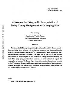
Here ak are coefficients which can be found in terms of the coupling constants tk of the tachyon operators and the chemical potential µ which fixes the Fermi level. Actually, they depend only on µ and the products λ2k = tk t−k . Instead, the “phases” αk are determined by ratios of the coupling constants. (Two of them can be excluded by constant shifts of ω and t.) It is easy to check that p(x, t) indeed satisfies (5.4) with u(x) = − 21 x2 . To get from this solution ϕ0 , note that p(x) is a two-valued function so that p± (x) can be identified with its two branches. As functions of ω they appear as follows. Let us define a ”mirror” parameter ω ˜ (ω, t) such that (see fig. 1) x(˜ ω (ω, t), t) = x(ω, t), ω ˜ 6= ω.
(5.6)
Then p+ can be identified with p and p− with p(˜ ω (ω, t), t). The solution for the background field is given again in the parametric form 1 ϕ0 (ω, t) = (p(ω, t) − p˜(ω, t)), 2
(5.7)
where we denoted p˜(ω, t) = p(˜ ω (ω, t), t) and ω is related to x by eq. (5.5). Due to (3.5), (5.1) and (5.7), the effective action (3.11) can now be rewritten as S(2) =
Z
dt
Z
i dx h (∂t η)2 + (p + p˜)∂t η∂x η + p˜ p(∂x η)2 . p − p˜
9
(5.8)
p
p (ω, t) ω
x ωsing(t)
ϕ0(ω, t) ∼ (ω, t) ω
p∼ (ω, t)
Figure 1: The Fermi sea of the perturbed MQM. Its boundary is defined by the two-valued function with two branches parameterized by p(ω, t) and p˜(ω, t). The background field ϕ0 coincides with the width of the Fermi sea.
5.2
Flat coordinates
We know from section 4 that any background described by the Das-Jevicki effective action leads to the flat target space metric. However, as we discussed above, the global structure of the target space can differ from that of the usual Minkowski space. To find whether this is the case, one should investigate the coordinate transformation mapping the target space metric into the standard form ηµν . In general, it is quite a difficult problem to find such a map explicitly. Remarkably, in our case given by the solution (5.5), this task can be accomplished. Indeed, we show in Appendix B that the change of coordinates from (t, x) to (τ, q) with τ =t−
ω+ω ˜ , 2
q=
ω−ω ˜ 2
(5.9)
brings the action (5.8) to the standard form S(2)
1 =± 2
Z
dτ
Z
i
h
dq (∂τ η)2 − (∂q η)2 ,
(5.10)
where the sign is determined by the sign of the Jacobian of the coordinate transformation (5.9). The Jacobian is defined by the function D in (B.2) and can be represented in the form 2D =
2(p − ξ)(˜ p − x˜t ) , p˜ − p
(5.11)
where ξ ≡ ∂t x(ω, t) and x˜t ≡ ξ(˜ ω, t) given explicitly in (B.4). The zeros of the Jacobian show where the map (5.9) is degenerate. All multipliers in (5.11) vanish at the line defined by the condition ω ˜ (ω, t) = ω or ∂x/∂ω = 0, which corresponds to the most left point of the Fermi sea where two branches of p(x) meet each other (see fig. 1). In terms of the flat coordinates (5.9), this line is given in the following parametric form τ = t − ωsing (t), 10
q = 0,
(5.12)
where ωsing (t) is a solution of the above condition. Also it defines the limiting value of the coordinate x, which should always be larger than xsing (t) = x(ωsing (t), t). However, the spacetime can be analytically continued through this line. This analytical continuation corresponds to that in all integrals x should run from ∞ to xsing and return back with simultaneous interchanging the roles of p and p˜. This shows that it is more natural to consider the plane of (t, ω) as the starting point rather than (t, x). The former is a twosheet cover of the physical region of the latter. ω appears as a parameter along fermionic trajectories and it should not be restricted to a half-line. Thus, we incorporate the whole scattering picture and glue two copies of the resulting flat spacetime together along the line (5.12). Unfortunately, there is an ambiguity in the choice of coordinates where the action has the form (5.10). Any conformal change of variables (5.9) (τ, q) −→ (u(t − ω), v(t − ω ˜ ))
(5.13)
leaves the action unchanged. Due to this we can find the form of the resulting spacetime only up to the conformal map. However, one can reduce the ambiguity imposing some conditions on the map (5.13). First of all, it should be well defined on the subspace which is the image of the (t, ω)-plane under the map (5.9), that is the functions u and v should not have singularities there. The next condition is the triviality of (5.13) in the absence of perturbations since in this limit (5.9) reduces to the well known transformation giving the flat Minkowski space [3]. Besides, we would like to retain the symmetry (t, ω) ↔ (−t, −ω) which is explicit when there are no phases αk in (5.5). It reflects the fact the our spacetime is glued from two identical copies (see discussion in the previous paragraph). This leads to the condition that u and v are odd functions. As a byproduct of our analysis we obtain also the conformal factor e2ρ appearing in (4.8). It should be found, in principle, from the condition of vanishing curvature for the metric Gµν . Instead, we get it as the Jacobian of the transformation√to the coordinates where√Gµν = ηµν . If u and v from (5.13) are such coordinates, than dtdx −G = dudv and, since −G = e2ρ , we conclude from (5.11) that e2ρ =
p˜ − p u′ v ′ . 2(p − ξ)(˜ p − x˜t )
(5.14)
The conformal factor becomes singular on the line (5.12) discussed above. However, this is only a coordinate singularity since it disappears after our coordinate transformation.
5.3
Structure of the target space
In this subsection we investigate the concrete form of the target space which is obtained as the image under the coordinate transformation trivializing the metric. From the previous subsection it follows that this transformation is a superposition of the map (5.9) and a conformal change of coordinates (5.13). Since the latter remains unknown, we will analyze only the image of the map (5.9). It will be sufficient to get a general picture because conformal transformations do not change the causal structure of spacetime. We restrict our analysis to the case of the simplest non-trivial perturbation with n = 1 in (5.5). It corresponds to the conformal Sine-Liouville theory. At R = 2/3 this theory is 11
τ
11111111111111111111111111111111111111111111111111 00000000000000000000000000000000000000000000000000 00000000000000000000000000000000000000000000000000 11111111111111111111111111111111111111111111111111 00000000000000000000000000000000000000000000000000 11111111111111111111111111111111111111111111111111 00000000000000000000000000000000000000000000000000 11111111111111111111111111111111111111111111111111 τ /q = 2R−1 00000000000000000000000000000000000000000000000000 11111111111111111111111111111111111111111111111111 00000000000000000000000000000000000000000000000000 11111111111111111111111111111111111111111111111111 00000000000000000000000000000000000000000000000000 11111111111111111111111111111111111111111111111111 00000000000000000000000000000000000000000000000000 11111111111111111111111111111111111111111111111111 00000000000000000000000000000000000000000000000000 11111111111111111111111111111111111111111111111111 00000000000000000000000000000000000000000000000000 11111111111111111111111111111111111111111111111111 00000000000000000000000000000000000000000000000000 11111111111111111111111111111111111111111111111111 00000000000000000000000000000000000000000000000000 11111111111111111111111111111111111111111111111111 ∆ 00000000000000000000000000000000000000000000000000 11111111111111111111111111111111111111111111111111 00000000000000000000000000000000000000000000000000 11111111111111111111111111111111111111111111111111 00000000000000000000000000000000000000000000000000q 11111111111111111111111111111111111111111111111111 00000000000000000000000000000000000000000000000000 11111111111111111111111111111111111111111111111111 00000000000000000000000000000000000000000000000000 11111111111111111111111111111111111111111111111111 00000000000000000000000000000000000000000000000000 11111111111111111111111111111111111111111111111111 00000000000000000000000000000000000000000000000000 11111111111111111111111111111111111111111111111111 00000000000000000000000000000000000000000000000000 11111111111111111111111111111111111111111111111111 00000000000000000000000000000000000000000000000000 11111111111111111111111111111111111111111111111111 00000000000000000000000000000000000000000000000000 11111111111111111111111111111111111111111111111111 00000000000000000000000000000000000000000000000000 11111111111111111111111111111111111111111111111111 00000000000000000000000000000000000000000000000000 11111111111111111111111111111111111111111111111111 00000000000000000000000000000000000000000000000000 11111111111111111111111111111111111111111111111111 00000000000000000000000000000000000000000000000000 11111111111111111111111111111111111111111111111111
Figure 2: Target space of the perturbed theory for the case R < 1. T-dual to the CFT suggested to describe string theory on the black hole background [15]. We also assume that the coefficients ak in (5.5) are positive what corresponds to the positivity of the coupling constants t±1 . It is the case which was considered in [9, 25, 10, 18, 26]. To find the image, we investigate the change of coordinates at infinity of the (t, ω) plane which plays the role of the boundary of the initial spacetime. In other words, we want to find where the boundary is mapped to. Thus we assume t and ω to be large and look at the dependence of ω ˜ of their ratio. At the asymptotics ω ˜ (ω, t) can be easily found, but the answer depends non-continuously on t/ω as well as on the parameter R. There are several different cases which we summarize in Appendix C. R ≥ 1: From the results presented in Appendix C it follows that in this case the image of the map (5.9) is the entire Minkowski spacetime. Thus, we do not see any effect of the tachyon perturbation on the structure of the target space. 1/2 < R < 1: In this case the resulting spacetime looks like two conic regions bounded by lines τ = ±(2R − 1)q ± R log aa01 (fig. 2). Near the origin the boundaries are not anymore the straight lines but defined by the solution of the following irrational equation ˜
˜
a0 eξ + a1 e(1−1/R)ξ = a0 eξ + a1 e(1−1/R)ξ ,
ξ˜ 6= ξ.
(5.15)
It allows to represent the boundary in the parametric form 1 ˜ q = (ξ − ξ(ξ)). 2
1 ˜ τ = − (ξ + ξ(ξ)), 2
(5.16)
Two conic regions are glued along some finite interval belonging to the τ -axis. It is just that line where the change of coordinates (5.9) is degenerate. We can easily find its length. As it was discussed in the previous subsection, the interval is defined by eq. (5.12). We need to find the limiting value of τ (t) when t → ∞. In this limit the condition for ωsing (t) can be written as 1 1 1 1 ∂x a1 e(1− R )ωsing + R t = 0 ⇒ ωsing (t) = t − ∆, ≈ a0 eωsing + 1 − 2 ∂ω R 2
�
�
12
(5.17)
where
R a0 ∆ = 2R log . 1 − R a1 �
�
(5.18)
Thus τ (t) −→ ∆/2 and we conclude that ∆ is the length we were looking for. t→∞ From this result it is easy to understand what happens when we switch off the perturbation. This corresponds to the limit a1 → 0. Then the interval ∆ (the minimal distance between two boundaries) logarithmically diverges and the boundaries go away to infinity. In this way we recover the entire Minkowski space. The similar picture emerges in the limit R → 1 when we return to the previous case R ≥ 1. It is interesting to look at the opposite limit where the length ∆ vanishes. It happens √ Ra0 when a1 = 1−R . The parameters are related to the coupling constant λ = t1 t−1 as follows [10] √ √ R−1 1 a0 = 2e− 2R χ , a1 = 2λe 2R2 χ , (5.19) where χ = ∂ 2 F /∂µ2 is the second derivative of the grand canonical free energy. This quantity is defined by the equation [9] 1
�
µe R χ − 1 −
2R−1 1 λ2 e R2 χ = 1. R
�
(5.20)
Taking into account (5.19) and (5.20), the condition of vanishing ∆ leads to the following critical point �� � 1 � 2R−1 2R 1 1 (5.21) −1 µc = − 2 − λ 2R−1 . R R In [10] it was shown that at this point the Fermi sea forms a pinch and beyond it the solution for the free energy does not exist anymore. Also this point coincides with the critical point of Hsu and Kutasov [27], who interpreted it as a critical point of the pure 2D gravity type. R = 1/2: This case can be analyzed using the result (C.1). We conclude that the spacetime takes the form of a strip bounded by lines τ = ± 12 log aa10 what agrees also with (5.18). R < 1/2: This interval of values of the parameter R was splited in Appendix C into two cases. However, they both lead to the same picture. Moreover, it coincides with one analyzed for 1/2 < R < 1 and shown in fig. 2. Nevertheless, there is an essential distinction with respect to that case. Using explicit expressions for the new coordinates from Appendix C, it is easy to check that the Jacobian of the transformation (5.9) is negative for R < 1/2. Therefore, one has to choose the minus sign in front of the action in (5.10). Due to this, the time and space coordinates are exchanged, so that τ and q are associated with space and time directions, correspondingly. As a result, the picture at fig. 2 should now be rotated by 90◦ .
5.4
Boundary conditions and global structure
We found that the introduction of tachyon perturbations in MQM is equivalent to consider string theory in the flat spacetime of the form described in the previous subsection (or its conformal transform). The main feature of this spacetime is the presence of boundaries. 13
Therefore, to define the theory completely, we should impose some boundary conditions on the fields propagating there. We do not see any rigorous way to derive them. Nevertheless, we discuss the most natural choices for the boundary conditions and their physical interpretation. Vanishing boundary conditions The most natural choice is to choose the vanishing boundary conditions. It can be justified by that the boundary on fig. 2 came from infinity on the (t, ω) plane of the matrix model. In the usual analysis of a quantum field theory one demands that all fields disappear at infinity. Therefore, it seems to be natural to impose the same condition in our case also. The presence of boundaries with vanishing conditions on them can be interpreted as if one placed the system between two moving mirrors. However, we note that such interpretation is reliable only for R < 1/2 where the boundaries are timelike. In the most interesting case R ∈ (1/2, 1) we would have to suppose that mirrors move faster than light. Nevertheless, this interpretation opens an interesting possibility. It is known that moving mirrors cause particle creation [19]. In particular, the resulting spectrum can be thermal so that the system turns out to be at a finite temperature. On the other hand, in [18] it was shown that the Sine-Liouville tachyon perturbation gives rise to the thermal description at T = 2π/R. Therefore, it would be extremely interesting to reproduce this result from the exact form of the spacetime obtained here. In our case the particle creation is a quite expected effect because two cones lead to the existence of two natural vacua associated with the right and left cone, correspondingly. When the modes, defining one of the vacua, propagate from one cone to another, they disperse on the hole and, in general, will lead to appearance of particles with respect to the second vacuum. The concrete form of the particle spectrum depends crucially on the exact behaviour near the origin since the creation happens only when the mirror is accelerated [28, 29]. Unfortunately, in this region the form of the boundary is known only inexplicitly through the equation (5.15). Besides, the situation is complicated by the possibility that one needs to make a conformal transform (5.13) to arrive to the flat coordinates. Usually, such transform can change thermal properties [14]. Therefore, it remains unsolved problem to check whether the particle creation in the found spacetime reproduces the result obtained in the MQM framework. Periodic conditions Although the vanishing boundary conditions are very natural, it is questionable to apply them in the case of spacelike boundaries. For example, this would lead to a discrete spectrum at finite distance from the origin although the spacelike slices are non-compact. In general, the situation when one encounters a boundary in time is very strange. Therefore, in this case it could be more natural to choose periodic boundary conditions where one identifies the upper boundary on fig. 2 with the lower one. As a result, the spacetime is compactified. For R ∈ (1/2, 1) the compact dimension is timelike so that we find closed timelike curves. Of course, their existence is a very bad feature. But it might be better than to have spacelike boundaries. For R < 1/2 the periodic boundary conditions can also be applied. Then the spacetime has the topology of a cylinder with a spacelike compact dimension and we do not encounter the above mentioned problems. In this case it is also expected that the change of radius of the cylinder in time will cause particle creation and can give rise to a temperature. 14
Note that the picture obtained in this case resembles the orbifold construction of [30], where the Minkowski spacetime was factored out by action of a discrete subgroup of boosts. It leads to four cones, joint at the origin, corresponding to the causal cones in the Minkowski spacetime. If one tries to interpret fig. 2 with the periodic boundary conditions following this analogy, one concludes that it corresponds to two cones of [30] (spacelike or timelike, depending on the value of R) with the resolved singularity because the cones are joint not at a point but along some finite interval. Twisted periodic conditions There is also another possible choice for the boundary conditions which comes from comparison with Matrix Quantum Mechanics. It is very unlikely that this possibility can be realized but we mention it for completeness. In MQM to define the density of states and, consequently, the free energy, one should place the system in a box and also impose some boundary conditions on the wave functions of fermions of the singlet sector of MQM. They relate the scattered (out-going) wave function to the in-coming one [10]. Thus one can say that they identify two infinities t, ω → ∞ and t, ω → −∞. Being applied to our picture, these conditions mean that one should identify the left lower boundary with the right upper one and vice-versa. In this way we arrive at the compactified spacetime but where it was “twisted” before the compactification. The topology of the resulting spacetime is that of the M¨obius sheet. Note that these boundary conditions have an advantage that they are invariant under the conformal map (5.13) if one required from it to preserve the symmetry (t, ω) ↔ (−t, −ω). However, the fact that they lead to a unorienetd spacetime rises doubts on their credibility. We stop our discussion at this point. We are not able to choose the right boundary conditions. Due to this, we are not able also to establish the effect produced by tachyon perturbations on the target space: either it is the appearance of boundaries or a compactification. But the form of the obtained spacetime indicates that one of these modifications of the global structure does take place.
6
Conclusions
We analyzed the proposal that the tachyon perturbations of 2D string theory in the linear dilation background have a dual description in a non-trivial target space. Comparing the Das–Jevicki collective field theory with the low-energy effective action of string theory, we found that the tachyon perturbations can not change the local structure of spacetime so that we always remain in the linear dilaton background. However, the relation between the flat coordinates, where the background metric has the standard Minkowski form, and the coordinates of the collective theory coming from Matrix Quantum Mechanics is affected by the perturbation. As a result, MQM describes only a part of the Minkowski spacetime. This introduces boundaries for the target space. But its real structure depends on the boundary conditions. If they are chosen to be the periodic conditions, we get a compactified target space. Unfortunately, we were not able to choose the correct boundary conditions and, therefore, we can not say what the final form of the target space is. One could ask about the physical meaning of the boundaries because the spacetime can be continued through them to get the entire Minkowski spacetime. However, when we work 15
with the tachyon perturbations in the framework of Matrix Quantum Mechanics, we can not access the parts of spacetime obtained by this continuation. The situation can be compared with that of the Unruh effect [31], when an accelerated observer “sees” only the Rindler cone of the Minkowski spacetime. Thus, we can think of the tachyon perturbations as if they place the system into another reference frame. However, there is a crucial difference between the Unruh effect and our situation. In the former case, the boundaries are lightlike and considered as event horizons, whereas our boundaries are spacelike or timelike and one should find for them a physical interpretation. In the context of string theory it is tempting to think about them as branes. Note that spacelike branes (S-branes) have also been introduced in string theory [32], so that the existence of spacelike boundaries should not be an obstacle for this interpretation. Recently, it was also suggested a relation between S-branes and thermodynamics [33]. May be one of the most interesting problems, which is left unsolved in the paper, is to show that the field-theoretic analysis on the found target space leads to a thermal description with the temperature 2π/R. This would confirm the result obtained in the MQM framework [18] and would be a non-trivial consistency check. Also, if the periodic boundary conditions are realized, it would be interesting to elaborate a connection with the work [30]. This might help to understand how to resolve the orbifold singularity of the type considered there. In [30] the resolution was found to be impossible. Finally, the main problem, which we did not consider here, is to find the string background corresponding to winding perturbations. The results obtained in this paper could be useful to approach the answer if one can realize the world sheet T-duality directly in the target space. Unfortunately, when the duality transformation does not act in the direction of a Killing vector, it is still an open problem. Acknowledgements: The author is grateful to V. Kazakov, I. Kostov and D. Vassilevich for very valuable discussions. This work was partially supported by European Union under the RTN contracts HPRN-CT-2000-00122 and -00131 and by European network EUROGRID HPRN-CT-1999-00161.
Appendix A. Perturbative solution of dilaton gravity We are interested in the solution of the system of equations (4.3) and (4.6). After the substitution T = eΦ η, they can be rewritten as
4α
′−1 Φ
1 − e−Φ β T − m2η η = ∇2 η = 0, 2 m2η = (∇Φ)2 − ∇2 Φ − 4α′−1 = 0,
β +
G βµν Gµν
−
4m2η G βµν
2
= 2∇ Φ − 4α
(A.1)
′−1 2Φ 2
e η = 0,
= Rµν + 2∇µ ∇ν Φ − ∇µ (eΦ η)∇ν (eΦ η) = 0.
Let us choose the conformal gauge Gµν = e2ρ ηµν .
16
(A.2)
Then in the light-cone coordinates X± =
X 0√ ±X 1 2
the equations take the following form
∂+ ∂− η = 0, ∂+ ∂− Φ − ∂+ Φ∂− Φ = 2α′−1 e2ρ , ∂+ ∂− Φ = −α′−1 e2(Φ+ρ) η 2 , 1 ∂+ ∂− ρ − ∂+ ∂− Φ = − ∂+ (eΦ η)∂− (eΦ η), 2 �2 1� ∂+ (eΦ η) , ∂+ ∂+ Φ = 2 �2 1� ∂− (eΦ η) , ∂− ∂− Φ = 2
(A.3)
where the last three equations are produced by the last equation in (A.1). First of all, it is easy to see that if η = 0, (4.7) is the unique solution. To generalize this statement, let us consider a solution which can be represented as an expansion around the linear dilaton background (4.7). We use the following ansatz ρ=
X
X 2 ǫk+1 φk , Φ = −√ ′ X1 + α k>0
ǫk+1 ρk ,
k>0
η=
X
ǫk ηk .
(A.4)
k>0
In the first order in ǫ we find (a) (b) (c) (d) (e) (f)
η1 = f1 (X+ ) + g1 (X− ), s
2 4 (∂+ − ∂− )φ1 = ′ ρ1 , ′ α α 4 1 1 −√ X ∂+ ∂− φ1 = − ′ e α′ η12 , α � � � � 1 − √2 ′ X 1 − √2 ′ X 1 α α η1 ∂− e η1 , ∂+ ∂− (ρ1 − φ1 ) = − ∂+ e 2 � � ��2 1 − √2 X 1 ∂+ e α′ η1 , ∂+ ∂+ φ1 = 2 � � ��2 1 − √2 ′ X 1 α ∂− e ∂− ∂− φ1 = η1 . 2 ∂+ ∂− φ1 −
(A.5)
Using equations (b) and (c), one can check that (d) is fulfilled identically. On the other hand, for (c), (e) and (f) to be consistent, some integrability conditions must hold. They are obtained comparing the derivatives of these equations. Taking into account (a), we get the following conditions on f1 (X+ ) and g1 (X− ) �
(f ′ − g ′ ) f ′ − �
(f ′ − g ′ ) g ′ +
q
2 (f q α′ 2 (f α′
�
+ g) = 0,
(A.6)
�
+ g) = 0.
The only solution of (A.6) is obtained when f ′ = g ′. Then we find α′ c21 − √4 ′ X 1 e α , ρ1 = 32
α′ c21 − √4 ′ X 1 1 (c1 X 0 + d1 )2 + e α , φ1 = 8 4 !
17
η1 = c1 X 0 + d1 ,
(A.7)
where c1 and d1 are some constants. In the second order we get the similar system of equations as (A.5), where one should change one of η1 in terms quadratic in tachyon by 2η2 . Then we obtain ρ2 =
4 1 α′ c1 c2 − √α′ X e , 16
φ2 =
1 4
�
(c1 X 0 + d1 )(c2 X 0 + d2 ) +
α′ c1 c2 4
0
η2 = c2 X + d2 .
�
− √4 ′ X 1
e
α
, (A.8)
But already in the next order in ǫ we encounter inconsistences which can not be overcomed. We must choose the vanishing tachyon and all other perturbations. Thus, we conclude that the only solution of the system (A.1), which can be represented in the form (A.4), is the linear dilaton background.
Appendix B. Change to the flat coordinates In this appendix we demonstrate that the quadratic part of the effective action for the tachyon field (5.8) in the coordinates (5.9) takes the form (5.10). First of all, for generic functions x, p and ω ˜ of ω and t the passage to the variables (5.9) leads to the action S(2)
1 = 2
Z
dτ
Z
dq
i |D| h A(∂τ η)2 − 2B∂τ η∂q η − C(∂q η)2 , p − p˜
(B.1)
where A =
h
ih
i
2 − ∂t ω ˜ − (∂ω x)−1 (1 + ∂ω ω ˜ ) (p − ∂t x) 2 − ∂t ω ˜ − (∂ω x)−1 (1 + ∂ω ω ˜ ) (˜ p − ∂t x) ,
B = ∂t ω ˜ (2 − ∂t ω ˜ ) − (∂ω x)−1 (p + p˜ − 2∂t x) (1 − ∂ω ω ˜ + ∂t ω ˜ ∂ω ω ˜) −2 + (∂ω x) (1 − ∂ω ω ˜ ) (1 + ∂ω ω ˜ ) (p − ∂t x) (˜ p − ∂t x) , C =
D =
h
∂t ω ˜ − (∂ω x)
−1
ih
(1 − ∂ω ω ˜ ) (p − ∂t x) ∂t ω ˜ − (∂ω x)
∂ω x . 1 − (∂ω ω ˜ + ∂t ω ˜)
−1
(B.2) i
(1 − ∂ω ω ˜ ) (˜ p − ∂t x) ,
From the explicit form (5.5) of p(ω, t) and x(ω, t) it is easy to check the following properties ∂x ∂x =p− , ∂t ∂ω with
∂ω ˜ p − x˜t ∂ ω ˜ = − ∂t p˜ − x˜t ∂ω
∂ω ˜ ∂x/∂ω = , ∂ω p˜ − x˜t
n 1 X k k x˜t ≡ ∂t x(˜ ω , t) = ω+ t . kak sinh (1 − )˜ R k=1 R R
"
#
(B.3)
(B.4)
These properties are enough to show that DA = DC = p − p˜ and B = 0 what gives the action (5.10).
18
Appendix C. Asymptotic values of the coordinates In this appendix we display the results for ω ˜ , τ and q as functions of t and ω which are obtained in the asymptotics t, ω → ∞ in the case of Sine–Liouville theory (n = 1). The results depend on the ratio t/ω as well as on the radius parameter. There are four different cases dependent of the value of R. We summarize them in four tables. In each table we distinguish several regions of t/ω. For each region we give the asymptotic expressions for the coordinates, the corresponding interval of values of τ /q, and the coefficients in front of the constant term log aa10 , which should be added to ω ˜ . The latter are given for ω > 0. For ω < 0 one should change their sign. R>1 t/ω
(−1, 1)
(1, ∞) ∪ (−∞, 1 − 2R) �
ω ˜ τ
−ω t
q τ /q log aa01
ω (−1, 1) 0
− 1 − R1 ω − R1 t � � 1 1 1 + 2R t − 2R ω �
1 (Rω + t) − R−1 1 ((2R − 1)t + ω) 2(R−1)
�
1 1 ω + 2R 1 − 2R t (1, 2R + 1) ∪ (2R + 1, ∞) ±1
1/2 < R < 1 t/ω (1 − 2R, 2R − 1)
ω ˜ τ q τ /q log aa01
(1 − 2R, −1)
�
−ω t ω (1 − 2R, 2R − 1) 0
1 2(R−1)
(2R − 1, 1)
((2R − 1)ω + t) (−∞, −1) R − R−1
(1, ∞) ∪ (−∞, 1 − 2R)
1 − 1−R (Rω − t) 2R−1 (ω − t) 2(1−R) 1 (ω − t) 2(1−R) ≈ (2R − 1) R − 1−R
�
�
1 R
− 1 ω + R1 t � � 1 1 − 2R (t − ω) 1 (ω − t) 2R ≈ (1 − 2R) ∓1
−
1/3 < R < 1/2 t/ω ω ˜ τ q τ /q log aa01
, 1 − 2R) ( (1−R)(1−2R) 1−3R 2 t 1−R R − 1−R t 1 t ω − 1−R
−ω +
(2R − 1, 1 − 2R) 0
(1 − 2R, 1)
1 − 1−R (Rω − t) 2R−1 2(1−R) 1 2(1−R)
(ω − t) (ω − t) ≈ (2R − 1) R − 1−R
) (1, ∞) ∪ (−∞, (1−R)(1−2R) 1−3R −
�
�
1 R
�
− 1 ω + R1 t 1 2R
�
(t − ω) (ω − t) ≈ (1 − 2R) ∓1
1−
1 2R
R < 1/3 t/ω ω ˜ τ q τ /q log aa01
( (1−R)(1−2R) , ∞) ∪ (−∞, 1 − 2R) 1−3R 2 t −ω + 1−R R − 1−R t 1 ω − 1−R t (R, 1 − 2R) ∪ (2R − 1, R) 0
19
(1 − 2R, 1)
1 (Rω − t) − 1−R 2R−1 (ω − t) 2(1−R) 1 (ω − t) 2(1−R) ≈ (2R − 1) R − 1−R
(1, (1−R)(1−2R) ) 1−3R �
�
− 1 ω + R1 t � � 1 1 − 2R (t − ω) 1 (ω − t) 2R ≈ (1 − 2R) −1
−
1 R
Finally, there are also two critical cases R = 1 and R = 21 . In these cases one can find explicitly the transformation of coordinates (5.9) on the entire plane. The results are R=1 ω ˜ = −ω τ =t q=ω
R = 1/2 +a1 e2t ω ˜ = −ω + log aa00+a −2t 1e a0 +a1 e2t 1 τ = t − 2 log a0 +a1 e−2t +a1 e2t q = ω − 21 log aa00+a −2t 1e
(C.1)
References [1] I. Klebanov, Lectures delivered at the ICTP Spring School on String Theory and Quantum Gravity, Trieste, April 1991, hep-th/9108019. [2] P. Ginsparg and G. Moore, “Lectures on 2D gravity and 2D string theory”, hep-th/9304011. [3] A. Jevicki, “Developments in 2D string theory”, hep-th//9309115. [4] S. Mukhi and C. Vafa, “Two dimensional black-hole as a topological coset model of c=1 string theory”, Nucl. Phys. B407 (1993) 667, hep-th/9301083. [5] D. Ghoshal and C. Vafa, “c=1 String as the Topological Theory of the Conifold”, Nucl. Phys. B453 (1995) 121, hep-th/9506122. [6] R. Dijkgraaf and C. Vafa, “N = 1 Supersymmetry, Deconstruction and Bosonic Gauge Theories”, hep-th/0302011. [7] V.A. Kazakov and A.A. Migdal, “Recent progress in the non-critical strings” Nucl. Phys. B311 (1988) 171. [8] R.Dijkgraaf, G.Moore, and M.R.Plesser, “The partition function of 2d string theory”, Nucl. Phys. B394 (1993) 356, hep-th/9208031. [9] V. Kazakov, I. Kostov, and D. Kutasov, “A Matrix Model for the Two Dimensional Black Hole”, Nucl. Phys. B622 (2002) 141, hep-th/0101011. [10] S.Yu. Alexandrov, V.A. Kazakov, and I.K. Kostov, “Time-dependent backgrounds of 2D string theory”, Nucl. Phys. B640 (2002) 119, hep-th/0205079. [11] G. Mandal, A. Sengupta, and S. Wadia, “Classical Solutions of Two-Dimensional String Theory”, Mod. Phys. Lett. A6 (1991) 1685. [12] E. Witten, “On String Theory And Black Holes”, Phys. Rev. D44 (1991) 314. [13] C.G. Callan, S.B. Giddings, J.A. Harvey, and A. Strominger, “Evanescent black holes”, Phys. Rev. D45 (1992) 1005, hep-th/9111056. [14] D. Grumiller, W. Kummer, and D.V. Vassilevich, “Dilaton Gravity in Two Dimensions”, Phys. Rep. 369 (2002) 327, hep-th/0204253. 20
[15] V. Fateev, A. Zamolodchikov, and Al. Zamolodchikov, unpublished. [16] E. Brezin, C. Itzykson, G. Parisi, and J.-B. Zuber, Comm. Math. Phys. 59 (1978) 35. [17] S.R. Das and A. Jevicki, “String field theory and physical interpretation of D = 1 strings”, Mod. Phys. Lett. A5 (1990) 1639. [18] S. Alexandrov and V. Kazakov, “Thermodynamics of 2D string theory”, JHEP 0301 (2003) 078, hep-th/0210251. [19] N.D. Birrell and P.C.W. Davies, Quantum Fields in Curved Space, Cambridge University Press, Cambridge, 1982. [20] J. Polchinski, “What is string theory”, Lectures presented at the 1994 Les Houches Summer School “Fluctuating Geometries in Statistical Mechanics and Field Theory”, hep-th/9411028. [21] R. Dijkgraaf, E. Verlinde, and H. Verlinde, “String propagation in a black hole geometry”, Nucl. Phys. B371 (1992) 269. [22] D. Gross and I. Klebanov, Nucl. Phys. B344 (1990) 475; Nucl. Phys. B354 (1990) 459. [23] D. Boulatov and V. Kazakov, “One-Dimensional String Theory with Vortices as UpsideDown Matrix Oscillator”, Int. J. Mod. Phys. 8 (1993) 809, hep-th/0012228. [24] J. Polchinski, String theory. An introduction to the Bosonic String, Vol. 1, Cambridge University Press, Cambridge, 1998. [25] S. Alexandrov and V. Kazakov, “Correlators in 2D string theory with vortex condensation”, Nucl. Phys. B610 (2001) 77, hep-th/0104094. [26] S.Yu. Alexandrov, V.A. Kazakov, and I.K. Kostov, “2D String Theory as Normal Matrix Model”, hep-th/0302106. [27] E. Hsu and D. Kutasov, “The Gravitational Sine-Gordon Model”, Nucl. Phys. B396 (1993) 693, hep-th/9212023. [28] G.T. Moore, “Quantum Theory of the Electromagnetic Field in a Variable-Length OneDimensional Cavity”, J. Math. Phys. 11 (1970) 2679. [29] S.A. Fulling and P.C.W. Davies, “Radiation from a moving mirror in two dimensional space-time: conformal anomaly”, Proc. Roy. Soc. London A348 (1976) 393. [30] N.A. Nekrasov, “Milne Universe, Tachyons, and Quantum Group”, hep-th/0203112. [31] S. R. Unruh, ‘’Notes on black hole evaporation”, Phys. Rev. D14 (1976) 870. [32] M. Gutperle and A. Strominger, ‘’Spacelike Branes”, JHEP 0204 (2002) 018, hep-th/0202210. [33] A. Maloney, A. Strominger, and X. Yin, ‘’S-Brane Thermodynamics”, hep-th/0302146.
21