Bayesian Calibration of Computationally ... - Cornell University

Bayesian Calibration of Computationally Expensive Models Using Optimization and Radial Basis Function Approximation Nikolai Blizniouk

∗

David Ruppert

Rommel Regis

§

Stefan Wild

¶

†

Christine Shoemaker Pradeep Mugunthan

‡

k

September 29, 2006

Abstract We present a Bayesian approach to model calibration when evaluation of the model is computationally expensive. Here, calibration is a nonlinear regression problem: given data vector Y corresponding to the regression model f (β), find plausible values of β. As an intermediate step, Y and f are embedded into a statistical model allowing transformation and dependence. Typically, this problem is solved by sampling from the posterior distribution of β given Y using MCMC. To reduce computational cost, we limit evaluation of f to small number of points chosen on a high posterior density region found by optimization. Then, we approximate the log-posterior using radial basis functions and use the resulting cheap-to-evaluate surface in MCMC. We illustrate our approach on simulated data for a pollutant diffusion problem and study frequentist coverage properties of credible intervals. Our experiments indicate that our method can produce results similar to those when the true “expensive” posterior is sampled by MCMC while reducing computational costs by well over an order of magnitude. ∗

Nikolai Blizniouk is a graduate student, School of Operations Research and Industrial Engineering, Cornell University, Rhodes Hall, Ithaca, NY 14853, USA. (E-mail: [email protected].) † David Ruppert is Andrew Schultz Jr. Professor of Engineering and Professor of Statistical Science, School of Operations Research and Industrial Engineering, Cornell University, Rhodes Hall, Ithaca, NY 14853, USA. (E-mail: [email protected].) ‡ Christine Shoemaker is Joseph P. Ripley Professor of Engineering, School of Civil and Environmental Engineering and School of Operations Research and Industrial Engineering, Cornell University, Hollister Hall, Ithaca, NY, 14853. (Email: [email protected].) § Rommel Regis is a Postdoctoral Associate, Cornell Theory Center, Cornell University, Rhodes Hall, Ithaca, NY, 14853. (Email: [email protected].) ¶ Stefan Wild is a graduate student, School of Operations Research and Industrial Engineering, Cornell University, Rhodes Hall, Ithaca, NY 14853, USA. (E-mail: [email protected].) k Pradeep Mugunthan is a Ph.D. graduate from Civil and Environmental Engineering, Cornell University, Ithaca, NY, 14853.

1

Keywords: computer experiments; design of experiments; interpolation; inverse problems; Markov Chain Monte Carlo; RBF; transformation.

1

INTRODUCTION

A common problem throughout science and engineering is the calibration of scientific models. Calibration means estimation of unknown parameters, for example, initial conditions or reaction or diffusion rates in a system modeled by partial differential equations. In this paper, we implement a Bayesian strategy for calibration when the models are specified by computationally expensive computer codes. Our focus is on computer codes that, in a single run, produce deterministic d-dimensional output vectors f (X, β) for all vector “indices” X in some specified set and a given parameter vector β. For example, the numerical solution of a partial differential equation produces output at all points on a space-time grid for a fixed vector of coefficients β. We assume that one has observed a sample Y1 , . . . , Yn of stochastic response vectors in Rd that correspond to the model values f (X1 , β), . . . , f (Xn , β), and the goal is to make inference about β. The vector Xi is assumed to be known to the experimenter and can thus be regarded as a label for the model f (Xi ; β) for Yi . We are motivated by environmental engineering problems where Yi ’s are vectors of observed concentrations of chemical species and Xi ’s are the temporal instants and spatial locations where the concentrations were measured, although our methodology is applicable to a wider range of problems. Evaluating f (X1 , β), . . . , f (Xn , β) for a single value of β can be computationally expensive taking, for example, 2.5 hours of CPU time in a groundwater bioremediation problem studied by Mugunthan, Shoemaker and Regis (2005) and Mugunthan and Shoemaker (2006, in press). Thus, accurate calibration of such models is infeasible without special methods such as those introduced here. Given that Yi is f (Xi , β (0) ) plus noise for value β (0) of β, calibration is seen to be a nonlinear regression problem. However, ordinary (nonlinear) least squares (OLS) is not recommended, since practitioners often find that the variation of Yi about f (Xi , β) is nonnormally distributed with nonconstant variance and correlated across time and space. We accommodate the nonnormality and heteroscedasticity by the transform-both-sides methodology of Carroll and Ruppert (1984) – we assume that, after a suitable transformation, Yi ’s are normally distributed and homoscedastic. To model dependence of Yi ’s, we use a 2

parametric space-time covariance model. Specifying the likelihood of the data Y1 , . . . , Yn and putting priors on parameters, we obtain the expression for the unnormalized posterior. Our algorithm has four main steps: (1) use numerical optimization to locate the region of the parameter space having high posterior probability; (2) evaluate the model on a suitable set of parameter values in the region of high posterior probability; (3) use the evaluations in steps (1) and (2) to construct a radial basis function (RBF) approximation to the log-posterior; and (4) draw a sample from the approximate posterior using a Markov Chain Monte Carlo (MCMC) algorithm. As a result, computational burden is reduced considerably since step (4) does not require expensive function evaluations. Using the sample from the approximate posterior allows us to solve the problems of Bayesian calibration and of prediction for F (β) by estimating moments and quantiles of the posteriors of β and F (β). Here, F is a function whose computation, for a given β, involves evaluation of f (·, β) for multiple values of X; more precisely, F (β) is the value of a functional of f (·, β). Empirical studies show that our algorithm can produce estimates of posterior densities for β and F (β) that are nearly the same as when sampling from the exact posterior. However, our methodology requires far fewer evaluations of the expensive function than would be needed if the exact posterior were sampled. This appears to be the first investigation that uses a direct nonparametric approximation to the posterior surface on the region of high posterior probability found by optimization. The introduction in Section 2.2 of a new transformation family, which is more attractive from the Bayesian perspective than the usual Box-Cox power family, allows a systematic treatment of data transformation, which is typically carried out in ad hoc fashion. As far as we are aware, this is also the first use of the transform-both-sides model with space-time correlation and should be of independent interest. The outline above reflects the organization of the paper: Section 2 specifies the statistical model for the data, Section 3 deals with the approximation to the posterior and contains details of the algorithm, Section 4 reports the results of a simulation study of a synthetic diffusion problem, and Section 5 discusses alternative approaches to calibration.

3

2

DESCRIPTION OF THE MODEL

2.1

A General Statistical Model

We assume that Yi is f (Xi , β) perturbed by noise, which could include model misspecification and measurement error. In many applications, the components of Yi show right-skewed variation about f (Xi , β) with variability that increases with f (Xi , β). The transform-bothsides (TBS) methodology of Carroll and Ruppert (1984, 1988) is particularly well suited for such data. Denote by Yi,j and fj (Xi , β) the jth components of Yi and f (Xi , β), respectively. Let {h(·, λ) : λ ∈ Λ} be a parametric family of differentiable increasing transformations indexed £ ¤ by λ. We assume that, for some λj , h(Yi,j , λj ) is distributed N h{fj (Xi , β), λj }, σj2 , where σj is constant as a function of Xi . Stated differently, h(·, λj ) is both a normalizing and variance-stabilizing transformation for Yi,j . In addition, we require that the Yi ’s can be transformed to have a joint multivariate normal (MVN ) distribution. In Section 2.2 we describe a new transformation family that we have used in our work. It is important to notice that both Yi,j and fj (Xi , β) are transformed in the same way. This implies that fj (Xi , β) is the conditional median of Yi,j given Xi , so, unlike when Yi,j alone is transformed as in Box and Cox (1964), fj (Xi , β) continues to be a model for Yi,j . In fact, the model for Yi,j is Yi,j = h−1 [h {fj (Xi , β), λj } + ²i,j , λj ] , where, for a fixed λ, h−1 (·, λ) is the inverse of h(·, λ), and ²i,j ∼ N (0, σj2 ). For example, if h(·, λj ) is the log transformation, then Yi,j = exp [log{fj (Xi , β)} + ²i,j ] = fj (Xi , β) exp(²i,j ), so the model has multiplicative, lognormal variation about the conditional median, fj (Xi , β). ¤T £ Let Y = Y1T , . . . , YnT be the nd-dimensional column vector of observed responses and ¤T £ f (β) = f (X1 , β)T , . . . , f (Xn , β)T be the corresponding value of the regression function. Define λ = (λ1 , . . . , λd )T , and denote by h{Y , λ} and h{f (β), λ} the coordinate-wise transformations of Y and f (β), where every coordinate corresponding to the jth outcome is transformed by h(·, λj ). Our statistical model is then h{Y , λ} ∼ M V N [h{f (β), λ}, Σ(θ)] 4

with the corresponding likelihood function ³ ´ exp −0.5kh(Y , λ) − h{f (β), λ}k2Σ(θ)−1 [Y |β, λ, θ] = · |Jh (Y , λ)|, (2π)nd/2 |Σ(θ)|1/2

(1)

where Jh (Y , λ) is the Jacobian of the transformation from Y to h{Y , λ} and Σ(θ) belongs to a family of covariance matrices parameterized by θ, as described in Section 2.3. Here we use the now standard notation that [list] is the joint density of the random variables in list and [list 1 |list 2 ] is the conditional density of the random variables in list 1 given those in list 2. We also use the conventional notation for the generalized norm, kxk2A = xT Ax. When the goal of the study is the posterior distribution of the value F (β) of some functional of f (·, β), as well as the posterior for β, it may be necessary to evaluate the expensive function for additional space-time indices Xn+1 , . . . , Xn∗ , for which no response Yi was observed, in order to compute or approximate F (β); further details are found in Section 3.3. We assume that, for a single value of β, a run of the expensive model produces the entire £ ¤T vector f ∗ (β) = f (β)T , f (Xn+1 , β)T , . . . , f (Xn∗ , β)T . This leads to computational savings, for example, in models relying on numerical meshes or grids, for which it is often more beneficial to obtain values of f (Xi , β) for all values Xi of interest in a single step rather than to compute them in two stages (i.e., first for f (β) and then for f (Xi , β) for all i > n). Once f has been evaluated at β (0) , [Y |β (0) , λ, θ] is usually a “cheap” function of (λ, θ), unless n is very large.

2.2

A New Transformation Family

The usual transformation family used with the TBS method is the Box-Cox family where hBC (y, λ) is (y λ − 1)/λ if λ 6= 0 and is log(y) = limλ→0 (y λ − 1)/λ if λ = 0. We assume that both the Yi ’s and f (X, β) are positive so the transformation should map the positive real number to the entire real line; otherwise, the transformation is to a truncated normal distribution. The only transformation in the Box-Cox family mapping (0, ∞) to (−∞, ∞) is the log transformation. Consequently, if one uses the Box-Cox family, one is assuming implicitly that the transformation is to a truncated normal distribution. (For discussion and examples, see Gelman, Carlin, Stern and Rubin (2004) and Thyer, Kuczera and Wang (2002).) Typically, practitioners ignore this fine point and approximate the truncated normal by a normal distribution. This results in an invalid statistical model since with positive probability the 5

noise term ²i,j added to hBC {fj (Xi , β), λj } produces values for which the inverse transfor−1 (·, λj ) is not defined. If one works with the truncated normal distribution, then mation hBC

the normalizing constant must be found by computing an nd-dimensional integral, which is likely to be difficult, if feasible, for all but the simplest models. Perhaps more importantly, the interpretation of Σ(θ) as a covariance matrix is lost when working with truncated distributions. It seems better to find a simple transformation family such that every transformation in it maps (0, ∞) to (−∞, ∞). We propose the COnvex combination of Identity and Log (COIL) family hC (y, λ) = λy + (1 − λ) log(y),

0 ≤ λ ≤ 1.

(2)

When λ is 0 or 1, then hC (·, λ) = hBC (·, λ). We will restrict λ to [0, 1), since hC (·, 1) does not map (0, ∞) to (−∞, ∞). Our simulation experiments show that the entire Box-Cox family for λ ∈ [0, 1) can be approximated well by our family; specifically, for each λ ∈ [0, 1) there are constants λ0 ∈ [0, 1) and a, b ∈ R such that hBC (y, λ) ≈ a + bhC (y, λ0 ) for a wide range of y values. The constants a and b do not play a role when the COIL transformation is combined with TBS since a is canceled out and b is absorbed into the variance parameter for identifiability. The inverse transformation h−1 C (·, λ) does not have a closed form but can be evaluated easily by interpolation. Generalization of the COIL family to include more severe concave transformations by taking convex combinations of, for example, the log transformation, the identity transformation, and hBC (·, −1), is possible but is not pursued here.

2.3

A Model for the Covariance

Define the noise vectors ²i = (²i,1 , . . . , ²i,d )T = h{Yi , λ} − h{f (Xi , β), λ} for i = 1, . . . , n, ²•,j = (²1,j , . . . , ²n,j )T , and ² = (²T1 , . . . , ²Tn )T . The covariance between ²i,j and ²i0 ,j 0 is modeled parsimoniously using a separable covariance function of the form C j,j 0 ·ρST (Xi , Xi0 ; γ), where C is a d × d covariance matrix for ²i and ρST (Xi , Xi0 ; γ) is a space-time correlation function parameterized by γ. One could consider nonseparable models if there were enough data, but in many applications a parsimonious model is highly desirable. Under some regularity conditions, misspecification of the covariance model will cause some inefficiency, but not 6

bias, in the estimation of β. For this reason we favor a parsimonious model over a more complex but more realistic model. In many if not most cases, ρST will also be separable, that is, the product of spatial and temporal correlation functions. Let S(γ) be the n×n space-time correlation matrix with S i,i0 (γ) = ρST (Xi , Xi0 ; γ). Then Var{²•,j } = C j,j · S(γ) and, more generally, Var{²} = Σ(θ) = S(γ) ⊗ C, where θ = (γ, C) and ⊗ denotes the Kronecker product of two matrices.

3

METHODOLOGY

3.1

An Approximation to the Posterior

Given a prior [β, λ, θ], one has a posterior [β, λ, θ|Y ] = R

[β, λ, θ, Y ] , [β, λ, θ, Y ] dβ dλ dθ

(3)

where [β, λ, θ, Y ] = [Y |β, λ, θ] · [β, λ, θ] is the joint density of the data and the parameters. (Recall the bracket notation for densities that was introduced in Section 2.1 following Equation (1).) In applications, β is the primary parameter and interest centers on its marginal posterior R [β|Y ] = [β, λ, θ|Y ] dλ dθ. Even though it may be infeasible to integrate out all of the nuisance parameters (λ, θ), it is often possible to integrate out some of them either analytically, by using conjugate priors as shown in Appendix A.4, or numerically. Let ζ be the subvector of (λ, θ) of remaining nuisance parameters after the integration. (This notation allows ζ to be (λ, θ) or be empty.) In what follows, Y is always regarded as fixed and [β, Y ] and [β, ζ, Y ] refer, respectively, to arbitrary unnormalized marginal and joint posteriors. If f were inexpensive to evaluate, then we could sample from [β, ζ|Y ] using [β, ζ, Y ] with a Metropolis-Hastings (M-H) algorithm, and then the sample of β would be a sample from [β|Y ]. However, drawing large samples is computationally prohibitive in our setting. Our goal is to obtain an accurate and cheap-to-evaluate nonparametric approximation to [β, Y ] or [β, ζ, Y ] based on a relatively small number of evaluations of f in order to use the resulting surface as a surrogate for the respective unnormalized posterior in a M-H algorithm, as the sampler does not require specification of normalizing constants. When the expression for [β, Y ] is not available, we approximate [β, Y ] heuristically first. For a fixed value of β, b let ζ(β) be the maximizer of [β, ζ, Y ] with respect to ζ. One possible approximation is the 7

profile posterior b πmax (β, Y ) = sup[β, ζ, Y ] = [β, ζ(β), Y ].

(4)

ζ

A more sophisticated Laplace approximation of Tierney and Kadane (1986) multiplies (4) by a correction factor. A simplification to (4), referred to as pseudoposterior, is obtained by b b β), b where (β, b ζ( b β)) b is the maximum a posteriori (MAP) estimator, the replacing ζ(β) by ζ( mode of the joint posterior [β, ζ|Y ]. All these approximations to [β, Y ] attempt to avoid the more difficult task of integrating out nuisance parameters by maximization with respect to them. It should be kept in mind, though, that neither the integration nor the maximization requires extra evaluations of f . In the sequel, the notation π(·, Y ) will be used to refer to any of these heuristic approximations to [β, Y ]. As a nonparametric approximation, we use interpolation of the logarithms of π(·, Y ) or [β, ζ, Y ] by radial basis functions (RBFs). We state our algorithm for π(·, Y ) as the surface of interest. The treatment of [β, ζ, Y ] is similar.

3.2

The Algorithm

In our algorithm, f ∗ is evaluated only during the optimization stage in order to find the MAP estimate (Step 1) and for values of β in a high posterior density region (Step 2) in order to approximate the logarithm of the posterior surface accurately by an RBF surface (Step 3). The approximate posterior surface is subsequently sampled using MCMC in Step 4. For ease of exposition, we assume that the posterior has a single mode located in the b but interior of the parameter space and that f is twice differentiable in a neighborhood β, we are currently generalizing the approach to multimodal posteriors. While selecting “design points” (the values of β at which to evaluate f ∗ ) we try to keep as small as possible the number of “uninformative” points – those very close to some point, at which the value of f ∗ is known, or far away from the mode. 3.2.1

Finding the MAP (Step 1)

For a given value β (0) of β, the gradient and Hessian of log{[β (0) , ζ, Y ]} with respect to ζ are available analytically, and so this function can be maximized efficiently to produce b (0) ) and thus to compute log{πmax (β (0) , Y )} from Equation (4). We perform this maxiζ(β mization using a constrained minimization routine (sequential quadratic programming) with 8

analytical gradients and Hessians, implemented in MATLAB in fmincon. Consequently, b ζ, Y ]} with rewe maximize log{πmax (β, Y )} with respect to β to find βb and then log{[β, b β) b and hence the MAP. The use of a gradient-based algorithm spect to ζ to determine ζ( for maximization with respect to β is not recommended unless the Jacobian of f comes at low cost along with f because finite differencing to estimate derivatives produces clusters of b ζ, Y ]} using publicly available software “uninformative” design points. We maximize log{[β, CONDOR described by Vanden Berghen and Bersini (2005), which implements a derivative-free trust-region algorithm UOBYQA of Powell (2000). 3.2.2

The Experimental Design (Step 2)

Ideally, we would like to fit the RBF surface over a highest posterior density (HPD) region of [β|Y ], defined as CR (α) = {β : [β, Y ] > κ(α)}, where κ(α) is chosen so that the credible region CR (α) contains the fraction 1 − α of the mass of [β, Y ]. Here α is a tuning parameter, for example, .05 or .01. The size (1 − α) HPD region cannot be computed accurately – not only for [β, Y ], but also for [β, ζ, Y ] and for any of the heuristic approximations to [β, Y ] from the previous section – without a prohibitive number of evaluations of f . We obtain an approximate b ζ), b which bR (α), using a Taylor expansion of log{[β, ζ, Y ]} near the MAP (β, HPD region, C corresponds to the approximation to [β, ζ|Y ] by a multivariate normal density. Specifically, b ζ). b let Ib be negative of the Hessian of log{[β, ζ, Y ]} with respect to (β, ζ) evaluated at (β, −1 By partitioning Ib into blocks corresponding to β and ζ one gets # " ββ βζ #! Ã" · ¸ βb Ib Ib β approx. , ∼ MV N , where ζβ ζζ ζ ζb Ib Ib " #−1 " ββ βζ # bββ Ibβζ −1 I Ib Ib Ib = = . ζβ ζζ Ibζβ Ibζζ Ib Ib

(5) (6)

Estimation of Ib by finite differences is wasteful as it does not produce new informative design points. We estimate Ib by fitting a quadratic surface to log{[β, ζ, Y ]} in a neighborhood of b ζ). b This procedure, stated in detail in Appendix A.1, allows one to reduce the number of (β, wasteful design points and to reuse the points from the optimization trajectory from Step 1. To avoid new notation, from now on we use the old notation for the true Ib and its blocks from Equation (6) to refer solely to the estimated Hessian and its blocks. 9

We define

½ bR (α) = C

¾ h i−1 T bββ 2 b b β : (β − β) I (β − β) ≤ χp,1−α ,

(7)

h i−1 ββ −1 b b b b b where I = I ββ − I βζ · I ζζ · I ζβ and χ2p,1−α is the (1 − α)th quantile of the χ2p distribution, with p being the dimension of β. This approximate HPD region is the size-(1 − α) minimum volume confidence ellipsoid for the (marginal) normal approximation to [β|Y ] based on Equation (5). We will use evaluations of f on this region at the same set of values of β to fit RBF surfaces to any of the posterior surfaces from Section 3.1, possibly all of them. This substep of determining an approximate design region is referred to as as Step 2A. We remark that Ib is crucial for subsequent analysis. If H is any square full-rank matrix ββ ββ such that Ib = HH T , for example, a Cholesky factor of Ib , then we apply the linear

transformation H −1 to β to ensure the same scale and to reduce correlation in parameters. Extra design points are chosen with respect to maximum separation criteria on this transformed space. We fit our RBF surface on the transformed space as well, but choose not to introduce new notation to emphasize this. Finally, Ib is also used in the MCMC stage to define one of the scale parameters of the proposal distribution. Let BO and BH be sets of values of β at which f ∗ is evaluated during optimization in Step 1 and during estimation of Ib in Step 2A, respectively. In general, points in BO ∪ BH bR (α) adequately to enable us to approximate the chosen posterior surface do not cover C accurately over the whole approximate HPD region. We augment these points with a spacefilling experimental design BE . Specifically, we require that points in BE be well-separated and do not lie close to those in BO ∪ BH , with between-point distances measured after the mentioned linear transformation. Details are provided in Appendix A.2. We refer to the step of choosing BE by Step 2B. bR (α0 ) for α0 ≤ α and define N = |BD |, the size of Finally, we let BD = (BO ∪ BH ∪ BE ) ∩ C BD . The points in BD will be used to build the RBF approximation. The motivation is that bR (α) rarely improve the quality the optimization trajectory points BO lying far outside of C of approximation, but can be a cause of numerical problems. We typically use α ≤ .1 and α0 = .01 or .005 in practice.

10

3.2.3

The RBF Approximation (Step 3)

We use radial basis functions (Buhmann 2003, Powell 1992) to approximate the logarithm of the posterior surface by an interpolant of l(·) = log{π(·, Y )} at the design points BD = {β (1) , . . . , β (N ) } of the form e l(β) =

N X

ai φ(kβ − β (i) k2 ) + q(β),

(8)

i=1

where β ∈ Rp , a1 , . . . , aN ∈ R, q ∈ Πpm (the space of polynomials in Rp of degree less than or equal to m), k · k2 denotes the Euclidean norm, and the basis function φ has one of the following forms: (1) surface spline: φ(r) = rκ , κ ∈ N, κ odd, or φ(r) = rκ log r, κ ∈ N, κ even; (2) multiquadric: φ(r) = (r2 + γ 2 )κ , κ > 0, κ 6∈ N; (3) inverse multiquadric: φ(r) = (r2 + γ 2 )κ , κ < 0; (4) Gaussian: φ(r) = exp(−γr2 ); where r ≥ 0 and γ is a positive constant. The purpose of the polynomial tail is to ensure that the interpolation matrix is invertible. In the numerical experiments, we use the cubic form φ(r) = r3 with a linear tail q(β) = (1, β T ) · c. Our choice of RBF interpolation over alternatives is motivated by the weakness of assumptions on the geometry of the interpolation points as compared, for instance, with those for multivariate polynomial interpolation (see Buhmann (2003, chap. 3)). This allows a greater re-use of the scattered design points from the optimization run. Another attractive feature is the ease of implementation of the RBF model; details are provided in Appendix A.3. Regis and Shoemaker (2006, in press) use RBF interpolation in global optimization of deterministic functions for the same reasons. 3.2.4

MCMC Sampling (Step 4)

In Step 4 of the algorithm we draw an MCMC sample from the density proportional to bR (α0 ), see the end of Secπ e(·, Y ) = exp{e l(·)} restricted to the approximate HPD region C tion 3.2.2 and Equation (8). This is done to prevent sampling π e(·, Y ) in the low-probability regions of [β|Y ] where π(·, Y ) is not approximated sufficiently well. We use the autoregressive Metropolis-Hastings (ARMH) algorithm of Tierney (1994) which does not require the normalizing constant of π e(·, Y ) to be known. The ARMH sampler uses a (vector) AR(1) process to generate candidate points β c given the current state β (t) of the chain, i.e., β c = µ + ρ(β (t) − µ) + et , where µ is the location parameter, ρ is the autoregressive parameter (matrix), and et ’s are i.i.d. noise vectors from a density g. The algorithm allows 11

much freedom in tuning its performance and includes the popular random walk M-H (when ρ = 1) and the independence M-H (when ρ = 0) algorithms as special cases. In our experiments, g is taken to be a finite mixture of multivariate normal and Student’s t-densities ββ centered at zero with dispersion matrices proportional to Ib . The location parameter µ is b We observed that negative values of ρ help to reduce serial correlation set to the MAP β. in the Markov chain. To improve mixing, we recommend that the tuning parameters for the sampler be calibrated to a particular application individually by conventional methods reviewed, for example, in Gelman et al. (2004), as at this stage MCMC does not require evaluations of f .

3.3

Bayesian Inference

Once the MCMC sample BM from the approximate posterior is obtained as discussed in Section 3.2.4, inference about β can proceed by standard methods. A problem of particular concern in environmental engineering is estimation of the value F (β) of some functional of f (·, β), for example, f (X, β) itself at values of X whose time coordinate is in the future. In this case, the set {F (β) : β ∈ BM } is a sample from the approximate posterior of F (β). Since F (β) is determined by f (·, β), it is also computationally expensive, and hence approximation is necessary to evaluate it at the points from the MCMC run. However, assuming as in Section 2 that F (β) is a function (or can be approximated by a function) of components of f ∗ (β), it may be sufficient to compute its values only on the approximate HPD region for β. Since we have already evaluated f ∗ at the design points in BD , it is cheap computationally to interpolate F (or an approximation to it) at the points in BD and to evaluate the resulting interpolant at the points in BM . This approximate sample from the posterior of F (β) can be subsequently used to estimate functionals of the posterior of F (β).

4

AN ENVIRONMENTAL APPLICATION

In this section, we consider calibration of an environmental model for the concentrations of pollutants and illustrate our methodology on a synthetic test problem. A test problem was chosen such that f (X, β) is given in closed form and can be evaluated inexpensively. Unlike with the expensive model functions used in many applications, this allows us to carry out an extensive Monte Carlo study comparing the coverage properties of the approximate Bayesian 12

credible intervals based on RBF surfaces that require a relatively small number of evaluations of f ∗ with those of the exact credible intervals that require thousands of evaluations of the expensive exact posterior. Examples of methods designed for calibration and uncertainty analysis of computationally expensive environmental models are Mugunthan et al. (2005) and Mugunthan and Shoemaker (2006, in press), respectively. The methods in both of these papers are applied to a remediation problem at US-DOD site that has been contaminated with chlorinated ethenes in the soil and groundwater. The simulation model there takes 2.5 hours to run. Neither of these earlier methods base analysis on the joint posterior density of the parameters as is done in this paper.

4.1

Environmental Assessment of a Chemical Spill: Formulation

Consider a chemical accident that has caused a pollutant to spill at two locations into a long and narrow holding channel. Assume it is known that the same mass M was spilled at each location (0 and L) and that the vector of the location and time of the first spill is (0, 0). However, the location L and time τ of the second spill are unknown as is the value of M and the diffusion rate D in the channel. We want to estimate the average concentration of the pollutant at the end of the channel and assess the uncertainty associated with this value since harmful effects to the environment are usually estimated from pollutant concentrations. We want to know the joint posterior distribution of all the parameters, but the parameter L is of special interest because L locates the as yet unidentified industry that will need to pay for its share of the clean-up costs. A first-order approach to modeling the concentration of substances in such channels is to assume that the channel can be approximated by an infinitely long one-dimensional system in which diffusion is the only transport device. We assume that the spills are each of mass M and occur instantaneously at space-time points (s, t) = (0, 0) and (s, t) = (L, τ ) and that the diffusion coefficient D is constant in both time and space. This leads to the concentration representation (for t > 0 and s ≥ 0): · 2¸ · ¸ M −s M −(s − L)2 C(s, t; M, D, L, τ ) = √ exp +p exp · I(τ < t), (9) 4Dt 4D(t − τ ) 4πDt 4πD(t − τ ) where I is the indicator function. We take β to be the vector of the four unknown environmental parameters (M, D, L, τ ) and consider the scaled concentration f {(s, t), β} = 13

√

4πC(s, t; β). We assume that each of the five monitoring stations fixed at spatial locations sj =

0, .5, 1, 1.5, 2.5 record 200 concentration readings at times tk = .3, .6, . . . , 50.7, 60. The corresponding expensive model function is f (β) = {f (X1 , β), . . . , f (X1000 , β)}T , where Xi = (sj , tk ) if i = (j − 1) · 200 + k. In this example f (Xi , β) is scalar because there is only one pollutant. The ultimate goal of the study is to assess the space-time prediction uncertainty associated with the average concentration at the end of the channel, corresponding to s = 3, over P the time interval [40, 140]. To this end we consider the function F (β) = 20 i=0 f {(3, 40 + 5i), β} which requires evaluation of f at the additional points {(3, 40), (3, 45), . . . , (3, 140)}. As discussed in Section 2, the expensive model that we evaluate is ¡ ¢T f ∗ (β) = f {β}T , f {(3, 40), β}, . . . , f {(3, 140), β} . An intermediate goal is estimation of the posterior density of β, which is partially captured by the marginal densities of its components. The vector Y of observed concentrations is generated according to the model given by Equations (1) and (9) with the value of λ = .333 for the COIL family given by Equation (2) and the values of β i ’s and respective parameter spaces (domains) given in Table 1. Notice that the likelihood from Equation (1) is discontinuous since C(si , tj ; β) in Equation (9) explodes when β 3 ≡ L = si and β 4 ≡ τ approaches tj from below. To avoid discontinuities, the parameter space for β 4 was restricted to the interval containing the true value of the parameter, given in Table 1. Components of Y are independent, with variance of h(Yi , λ) for every i equal to the sample variance of h{f (X1 , β), λ}, . . . , h{f (X1000 , β), λ}, computed for the true (fixed) values of β and λ and multiplied by a scaling constant c2 . Here, c controls the amount of noise in the transformed observed data relative to the variability of the corresponding transformed model values. For illustrative purposes – to ensure that the likelihood has a single dominant mode – c is set to .3. We put a uniform prior on (β, λ) over the parameter spaces mentioned earlier and an overdispersed inverse-gamma prior on σ 2 . This is a special case of the earlier model for multiple chemical species, and, as shown in Appendix A.4, σ 2 can be integrated out analytically. Thus [β, λ, Y ] is the unnormalized posterior from which we derive π(·, Y ) as discussed in Section 3.1. 14

4.2

Analysis

We applied our algorithm to a large number of dataset replications with the same statistical b λ) b model and parameter values but a different realization of the noise. The maximizer (β, of [β, λ, Y ] was found by CONDOR via maximization of πmax (·, Y ) given by Equation (4), and Ib was estimated by fitting a quadratic, as explained in Sections 3.2.1 and 3.2.2 and Appendix A.1. The mean and standard deviation of the number of function evaluations to find the MAP when started at a random point from the uniform distribution on the parameter space were around 100 and 20, respectively. Nearly all of the points in BO produced in Step 1 were sufficiently separated to be used as part of the experimental design. However, usually just over one third of them were actually valuable for Hessian estimation or surface bR (α0 ) and hence too far away from the mode. approximation while the rest were outside of C Based on 1000 dataset replications, the mean and median numbers of new design points to estimate Ib by fitting a quadratic, including the 8 points corresponding to forward differencing to obtain an estimate of the diagonal, were 20 and 19, respectively. A small correlation −1 between β and λ and small variance of λ, as estimated by the entries of Ib , indicate that b Y ]. [β|Y ] is likely to be close to the conditional density [β|λ = λ, bR (α) given by Equation (7), with α in Experiments were run for elliptical design regions C {.2, .1, .05, .01} and numbers of extra experimental design points (|BE |) in {0, 10, 20, . . . , 100}. It was observed that the estimates of the posterior densities based on MCMC samples from bR (α) provided there are enough approximate surfaces are not very sensitive to the size of C extra design points, with larger regions requiring greater numbers of extra design points. Also, for a fixed α, there is usually little (visual) improvement in density estimates when the size of BE grows above 50, and the quality of approximation is often unsatisfactory for the sizes of BE below 20. All graphical summaries of posterior densities for β and F (β) that we report for a single bR (.1) region with 30 extra design points for β, representative dataset correspond to the C the same for every surface. In the case of RBF interpolation of log{[β, λ, Y ]}, for each β (i) ∈ BD , we choose 10 design points for λ and fit the RBF surface at the design points {(β (i) , λij ) for i = 1, . . . , N and j = 1, . . . , 10}, chosen as outlined in Appendix A.2. All tabular summaries pertain to this RBF approximation to [β, λ, Y ] and the true surface [β, λ, Y ]. All results are reported for the ARMH sampler with ρ = −0.25, the density g 15

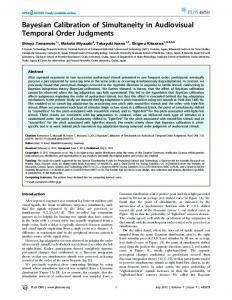
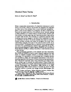
being the equal-weight mixture of a multivariate normal and Cauchy distributions and with other parameters chosen as discussed in Section 3.2.4. Figure 1 overlays plots of kernel density estimates for the components of β using MCMC samples of size 30,000 from the RBF approximations to the pseudoposterior, the profile posterior (with and without Laplace correction) and to the joint posterior. The close agreement b Y] among the curves supports the conjecture that the approximation of [β|Y ] by [β|λ = λ, is meaningful for this test problem. The plots of the estimates of the marginal densities of β i ’s based on a M-H sample of the same length from the exact unnormalized joint posterior [β, λ, Y ], also on the same figure, confirm the validity of findings. Of course, in practice we would not be able to visualize the true surface in the way we do it here due to computational limitations. Samples from the approximate posterior of F (β) were obtained by first interpolating F at β ∈ BD by the (cubic) RBF surface of the form given by the right-hand side of Equation (8) and then evaluating the resulting interpolant at the MCMC samples from the approximate surfaces stated in the previous paragraph; see Section 3.3 for discussion. Likewise, the sample from the true posterior of F (β) was obtained by evaluating F at the sample from [β|Y ]. Striking similarity between the exact and RBF results in Table 1 and in Figure 2 suggest that our method is capable of achieving nearly the full accuracy of estimation at the expense of only a small fraction of the computational cost required to carry out MCMC sampling using the exact posterior surface. Another important criterion for the assessment of the methodology concerns examination of the coverage properties of the Bayesian credible intervals for the components of β and for F (β) based on our approximations. We believe that if the final goal is a credible interval for F (β), then a very accurate approximation to the posterior of β is unnecessary, and a credible interval based on a less accurate approximation (requiring a smaller number of extra design points) is likely to have similar coverage properties to those of the credible interval based on the corresponding true posterior. Below we report findings of the following study: for each of the 1000 replications of Y under the same model and parameter values but a different realization of noise, we find the MAP and estimate Ib as before. We then take an MCMC sample of size 10,000 using the bR (.1) true surface [β, λ, Y ] and the respective RBF surface with approximate HPD region C and the number of extra experimental design points |BE | = 30. Reported in Table 2 are the 16

observed coverage proportions of the components β ∗i of the true value of β by symmetric credible intervals of sizes .9, .95 and .99 obtained from the MCMC samples, along with the corresponding standard errors. The last three columns of Table 1 give means and standard deviations for the ratios of the lengths of RBF and exact credible intervals over all datasets. The outcomes of the experiment allow one to conclude that the coverage properties of the credible intervals based on exact and approximate surfaces are similar, and that the respective interval lengths are close. The tables also suggest that the approximate credible intervals act as reasonable substitutes for frequentist confidence intervals, as the observed coverage proportions are close to the nominal sizes of the confidence intervals.

5 5.1

DISCUSSION Survey of Literature

Literature dealing with Bayesian calibration and prediction of output of complex computer models focuses on reduction of the number of expensive function evaluations via approximation of f rather than of the posterior. Papers by O’Hagan, Kennedy and Oakley (1998) and Kennedy and O’Hagan (2000) assume that the model can be run at different levels of complexity, which they use to build a Markov-type model for dependence between consecutive levels of the code and to utilize the cheaper lower levels of the code to help predict the expensive top-level code output. (In Kennedy and O’Hagan (2001), the unobservable physical model, approximated by a complex code, plays the role of the top-level code.) Under a similar assumption that the computer code can be “coarsened”, in particular, to lower the dimension of input (β in our notation), Higdon, Lee and Holloman (2002) run coarse and fine (corresponding to the original expensive model) Markov chains in tandem and use information from the faster-mixing coarse chain to improve mixing of the fine chain. A recent paper of Christen and Fox (2005) proposes to use a cheap-to-evaluate approximation to the unnormalized posterior density, which is assumed to be available, to evaluate the expensive posterior only for the MCMC moves that are likely to be accepted. The emphasis, however, is on the models for which approximation to the posterior is obtained by replacing f by an approximation, for example, by linearization.

17

5.2

Differences from Earlier Approaches

The route we take is significantly different from those mentioned. First, we are not assuming that the “black-box” f can be opened to produce an inexpensive approximation to the expensive code. Second, given our interest in the sample from the posterior for β, we approximate the (scalar-valued) posterior directly, and not through approximation of the high-dimensional model output f . Third, we realize that in many problems sampling thousands of times from the exact posterior is not computationally feasible and thus work solely with the approximation, unlike Higdon et al. (2002) and Christen and Fox (2005). For problems in which the approach of the latter two authors is feasible, our RBF approximation can be modified (by adding more mass to the tails of π e(·, Y )) to provide an initial approximation to the exact posterior that can be gradually refined as more expensive code evaluations are made in the course of sampling.

5.3

Computational Issues

Over a number of dataset replications, the results indicate that our method can produce results similar to those that require MCMC sampling of the exact posterior surface, but with far fewer computationally expensive functions evaluations. Using an average number of 150 function evaluations, our method produces estimates of posterior densities for β and F (β) that are nearly the same as those obtained at the cost of 30,000 evaluations of f ∗ incurred when sampling from the exact posterior. Since f ∗ is a computationally expensive function, the total computation times for solving the problem are based almost entirely on the number of function evaluations. The number of function evaluations is |BO | + |BH | + |BE |; recall definitions in Sections 3.2.1 and 3.2.2. These evaluations of f ∗ take place in Step 1 when optimization is used to find the MAP and in Step 2 when an improvement in the accuracy of the approximation of the logarithm of posterior surface is obtained by doing additional function evaluations in a high-probability neighborhood of the maximizer. The time for other computational steps including fitting the RBF, setting up the optimization algorithm to find the next design point, and performing all the calculations in Steps 3 and 4 take a tiny fraction of the computational time required for the evaluations of f ∗ . In contrast to typical optimization searches, here we want to use the function evaluations 18

generated during the optimization search not only to find the maximizer, but also to help characterize the function around the maximizer. We then “re-use” the function evaluations from the optimization search to build an RBF surface. We use derivative-free optimization methods that generate design points, at which f ∗ is evaluated, that are a reasonable distance apart. Our experience with derivative-based optimization for our example was that many of the design points were so close to each other that they were not carrying much new information about the surface values (in addition to that provided by their neighbors) and that they could not all be used in RBF interpolation without creating numerical instabilities.

5.4

Conclusions

This paper presented a Bayesian solution to calibration problem when the feasible number of evaluations of the computationally expensive model is relatively small and no cheapto-evaluate approximation to the computer model is available. Sampling from the exact expensive posterior using MCMC is questionable under such restrictions. Indeed, the computational budget may not be sufficient to ensure both that the Markov chain gets close to its limiting distribution and that the sample is “informative” about β if the Markov chain mixes slowly. The main contribution is the algorithm of Section 3.2, which re-uses a subset of design points from a derivative-free optimization search, augmented with additional design points, to build an RBF approximation for the posterior on the region of high posterior probability. This allows one to draw arbitrarily long samples from the cheap proxy to the true expensive posterior. Our results required, on average, 150 evaluations of f ∗ , which is less than 1/60 of the 10,000 evaluations used by the MCMC procedure that samples the exact posterior. (Of course, fewer iterations could be used, but this would noticeably increase Monte Carlo error.) This difference is very significant for computationally expensive functions for which many thousands of evaluations are infeasible. Our method hence shows promise as a means for doing a rigorous Bayesian uncertainty analysis on some functions (including simulation models) for which there currently does not exist a numerically feasible alternative method.

5.5

Further Developments

Our current work focuses on extending the approach to deal with f under less restrictive smoothness assumptions, posteriors with multiple important modes and pronounced skew19

ness, and on developing a sequential procedure for determining an approximate HPD region and an experimental design on it. A systematic study of the effect of space-time dependence is also needed. After more insight into these issues is gained, the methodology will be applied to a truly expensive model.

ACKNOWLEDGMENTS The research of Blizniouk was supported by the National Science Foundation under grant DMS-04-538 (PI’s Ruppert and Shoemaker). Research of Wild was supported by a Department of Energy Computational Science Graduate Fellowship, grant number DE-FG0297ER25308. Regis was supported by NSF grant CCF-0305583 (PI Shoemaker) and Mugunthan on NSF grant BES-0229176 (PI Shoemaker). Ruppert and Shoemaker were also partially supported on the grants on which they are PI’s.

A A.1

APPENDIX Estimation of Ib

Let p = dim(β) and u = dim(ζ). To approximate the Hessian Ib of − log{[β, ζ, Y ]} at b ζ) b by forward differences generally requires (around) (p + u + 1)(p + u + 2)/2 function (β, evaluations. Partition Ib as in Equation (6). In our problem, Ibζζ can be found analytically, and the off-diagonal blocks of Ib can be computed entirely from the evaluations of f used to estimate the diagonal of Ibββ . Unfortunately, the (p + 1)(p + 2)/2 points for evaluation of f by finite differences to compute Ibββ are very close to βb and are not valuable for surface approximation. However, one can lower the number of uninformative design points using the approach below. b β), b Y ]} ≈ const − 1 kβ − βk b 2 Taylor’s theorem suggests an approximation log{[β, ζ( 2

b 2 on the ellipsoid E(c) = {β : kβ−βk Ib

ββ

Ibββ

2

≤ c } for some c. We propose to choose (p + 1)(p + 2)/2

design points that are well-separated inside E(c), fit a quadratic surface through them and estimate Ibββ by the Hessian of the quadratic. The task is to ensure that these points lie inside E(c) without knowing the shape and orientation of the ellipsoid. Denote by ei the ith standard basis vectorqfor Rp and notice that the boundary of E(c) passes through points βb ±bi , where bi = ei · c/ Ibββ (i, i) and Ibββ (i, i) is the ith diagonal entry of Ibββ . The convex 20

hull of these points ½ ¾ P P2 Pp β : β = βb + pi=1 (ψi,1 − ψi,2 )bi such that ψ = 1 i,j j=1 i=1 H(c) = and ψi,j ≥ 0 for i = 1, . . . , p and j = 1, 2 is a subset of E(c), and so it is guaranteed that any experimental design on H(c) also lies in E(c). Hence one only needs to estimate the diagonal of Ibββ by forward differences using at most 2 · p extra function evaluations, half of which are reused in computation of the offdiagonal blocks Ibβζ . (Thus we have reduced the number of “uninformative” design points roughly by (p + 1)(p − 2)/2.) The argument c in the definition of the ellipsoid is to be chosen by the experimenters in accord with their beliefs. It is helpful to think of c2 as a quantile of the χ2p distribution that b Y ]. defines a confidence ellipsoid for the multivariate normal approximation to [β|ζ = ζ, Large values of c often yield Hessians that are inaccurate or not positive definite, and very b We had some success with the following small values result in new design points close to β. procedure to estimate Ib and to produce the set BH from Section 3.2.2: 1. Initialization: q (a) Choose a moderate initial value of c, say,

χ2p,0.1 .

(b) Set BH = BO and remove from BH points very close to each other. The set BH will contain values of β for which f ∗ has been computed. Assume for now that |BH | ≤ (p + 1)(p + 2)/2. 2. Augment BH with new well-separated points so that |BH ∩ H(c)| = (p + 1)(p + 2)/2 and evaluate f ∗ at the new points. 3. Fit a quadratic surface through the points in BH ∩ H(c) and plug its Hessian into the b If the resulting estimate of Ib (not only that of Ibββ ) is not positive expression for I. definite, reduce c and return to the previous step. Otherwise terminate; return Ib and (the set difference) BH = BH − BO . If |BH | > (p + 1)(p + 2)/2 in step 1(b) above, then no new design points are necessary and one starts by working with subsets of BH . Once they are exhausted, one moves to Step 2.

21

A.2

Choice of Design Points

While forming BH and BE , we require that the new design points lie far from each other and from the points where f ∗ has been evaluated previously (“fixed points”). This objective is related to the maximin criterion that attempts to max imize the minimum between-point distance over all pairs of design points (Santner, Williams and Notz (2003, sec. 5.3)). Generating such designs exactly is computationally difficult, and usually one is happy to obtain a good approximate maximin design (Trosset 1999). We devised a simple “greedy” algorithm to update the set of fixed points with NE extra design points: (i) choose κ > 1 and draw dκ · NE e candidate points uniformly at random on the design region; (ii) at the jth iteration, find the pair of points closest to each other that has at least one candidate point; if it has a single candidate point, delete it, otherwise delete the one that is closest to the remaining (fixed and candidate) points, until only NE candidate points remain. This algorithm is applied to update BO to produce BH and then to augment BO ∪ BH with BE . As an intermediate step, one has to sample uniformly inside polytopes and spheres; for discussion, see Devroye (1986, chap. 5). To obtain the (joint) experimental design for β and ζ for fitting an RBF surface to bR (α) as in Section 3.2.2 and auglog{[β, ζ, Y ]}, we start with a (marginal) design for β on C ment each design point β (i) ∈ BD with a (conditional) design for ζ based on the multivariate normal approximation to [ζ|β = β (i) , Y ], derived from Equation (5). As a consequence, the increase in the dimension of the argument of the posterior (going from π(·, Y ) to [β, ζ, Y ]) in this problem need not translate into the increase in the number of evaluations of f .

A.3

Details for Fitting the RBF Surface

We now describe the procedure for fitting the RBF interpolation model of Section 3.2.3 with the cubic basis function and a linear polynomial tail q(β) = (1, β T ) · c. Discussion of fitting for other choices of basis functions is in Powell (1996). Define the matrix Φ ∈ RN ×N by: Φi,j = φ(kβ (i) − β (j) k2 ), for i, j = 1, . . . , N . Let P ∈ RN ×(p+1) be the matrix with (1, {β (i) }T ) as the ith row for i = 1, . . . , N . The coefficients for the RBF surface that interpolates l(·) = log(π(·, Y )) at the points β (1) , . . . , β (N ) are obtained by solving the system µ

Φ P PT 0

¶µ

a c

¶

22

µ =

L 0

¶ ,

(10)

h iT where L = l(β (1) ), . . . , l(β (N ) ) , a ∈ RN and c ∈ Rp+1 . Our RBF interpolation model is a form of universal kriging with generalized covariances, as the above RBF interpolation equations are identical to the dual-kriging equations (Cressie 1991, sec. 4.4.5). The coefficient matrix in Equation (10) is invertible if and only if the rank of P is p + 1 (Powell 1992). For stability purposes, we solve Equation (10) by means of the matrix factorizations, as described in Powell (1996).

A.4

Details on Integrating C out

Let Z = Z(β, λ) be the matrix with the ith row [h{Yi , λ} − h{f (Xi , β), λ}]T for i = 1, . . . , n, e = R−T Z. Notice that, under the R be the upper-triangular Cholesky factor of S(γ) and Z separable covariance model Σ(θ) = S(γ) ⊗ C of Section 2.3, the likelihood equation (1) e 1,• , . . . , Z e n,• of Z e are i.i.d. M V N (0, C). Notice that implies that the rows Z [Y |β, λ, (γ, C)] ∝ |Jh (Y ; λ)| · |S(γ)|

−d/2

|C|

−n/2

n Y

³

e j,• k2 −1 exp −0.5 · kZ C

´

j=1

³ ´ e T Z} e . = |Jh (Y ; λ)| · |S(γ)|−d/2 |C|−n/2 exp −0.5 · tr{C −1 Z We put a Wishart prior on C −1 and assume that, a priori, C and (β, λ, γ) are independent, so that ¡ ¢ [β, λ, γ, C −1 ] ∝ |∆|a |C −1 |a−(d+1)/2 exp −tr{∆C −1 } · [β, λ, γ], where a > (d − 1)/2, ∆ ∈ Md , the space of d × d symmetric positive definite matrices, and tr(·) is the trace operator. This allows us to integrate C out of the joint posterior analytically: Z [Y |β, λ, (γ, C)] · [β, λ, γ, C −1 ]dC −1 Md Z ³ ´ e T Z/2 e + ∆)} |C −1 |a+(n−d−1)/2 dC −1 exp −tr{C −1 (Z ∝ c(β, λ, γ)

[β, λ, γ, Y ] =

Md T

e Z/2 e + ∆|−(a+n/2) ∝ c(β, λ, γ) · |Z = [β, λ, γ] · |Jh (Y ; λ)| · |S(γ)|−d/2 · |Z T [S(γ)]−1 Z/2 + ∆|−(a+n/2) .

23

References [1] Box, G. E. P., and Cox, D. R. (1964), “An Analysis of Transformations”, Journal of the Royal Statistical Society, Series B, 26, 211–246. [2] Buhmann, M. D. (2003), Radial Basis Functions, New York: Cambridge University Press. [3] Carroll, R. J., and Ruppert, D. (1984), “Power Transformation When Fitting Theoretical Models to Data”, Journal of the American Statistical Association, 79, 321–328. [4] ————– (1988), Transformation and Weighting in Regression, New York: Chapman & Hall. [5] Christen, J. A., and Fox, C. (2005), “Markov Chain Monte Carlo Using an Approximation”, Journal of Computational & Graphical Statistics, 14, 795–810. [6] Cressie, N. (1991), Statistics for Spatial Data, New York: Wiley. [7] Devroye, L. (1986), Non-Uniform Random Variate Generation, New York: SpringerVerlag. [8] Gelman, A., Carlin, J. B., Stern, H. S., and Rubin, D. B. (2004), Bayesian Data Analysis (2nd ed.), Boca Raton: Chapman & Hall/CRC. [9] Higdon, D., Lee H., and Holloman, C. (2002), “Markov Chain Monte Carlo-Based Approaches for Inference in Computationally Intensive Inverse Problems”, in Bayesian Statistics 7, eds. J. M. Bernardo, J. O. Berger, A. P. Berger and A. F. M. Smith, pp. 181–197. [10] Kennedy, M. C., and O’Hagan, A. (2000), “Predicting the Output From a Complex Computer Code When Fast Approximations are Available”, Biometrika, 87, 1–13. [11] ————– (2001), “Bayesian Calibration of Computer Models”, Journal of the Royal Statistical Society, Series B, 63, 425–464. [12] Mugunthan, P., Shoemaker, C. A., and Regis, R. G. (2005), “Comparison of Function Approximation, Heuristic and Derivative-Based Methods for Automatic Calibration of 24

Computationally Expensive Groundwater Bioremediation Models”, Water Resources Research, 41, W11427, doi:10.1029/2005WR004134. [13] Mugunthan, P. and Shoemaker, C. A. (2006, in press), “Assessing the Impacts of Parameter Uncertainty for Computationally Expensive Groundwater Models”, Water Resources Research. [14] O’Hagan, A., Kennedy, M. C., and Oakley, J. E. (1998), “Uncertainty Analysis and Other Inference Tools for Complex Codes”, in Bayesian Statistics 6, eds. J. M. Bernardo, J. O. Berger, A. P. Berger and A. F. M. Smith, pp. 503–524. [15] Powell, M. J. D. (1992), “The Theory of Radial Basis Function Approximation in 1990”, in Advances in Numerical Analysis, Volume 2: Wavelets, Subdivision Algorithms and Radial Basis Functions, ed. W. Light, New York: Oxford University Press, pp. 105–210. [16] ————– (1996), “A Review of Algorithms for Thin Plate Spline Interpolation in Two Dimensions”, in Advanced Topics in Multivariate Approximation, eds. F. Fontanella, K. Jetter and P. J. Laurent, River Edge, NJ: World Scientific Publishing, pp. 303–322. [17] ————– (2002), “UOBYQA: Unconstrained Optimization by Quadratic Approximation”, Mathematical Programming, 92, 555–582. [18] Santner, T.J., Williams, B.J. and Notz, W. (2003), The Design and Analysis of Computer Experiments. New York: Springer–Verlag. [19] Regis, R.G., and Shoemaker, C.A. (2006, in press), “A Stochastic Radial Basis Function Method for the Global Optimization of Expensive Functions,” INFORMS Journal of Computing. [20] Tierney, L. (1994), “Markov Chains for Exploring Posterior Distributions,” The Annals of Statistics, 22, 1701–1786. [21] Tierney, L., and Kadane, J. B. (1986), “Accurate Approximations for Posterior Moments and Marginal Densities,” Journal of the American Statistical Association, 81, 82–86. [22] Thyer, M. A., Kuczera, G., and Wang, Q. J. (2002), “Quantifying Parameter Uncertainty in Stochastic Models Using the Box-Cox Transformation,” The Journal of Hydrology, 265, 246–257. 25

[23] Trosset, M. W. (1999), “Approximate Maximin Distance Designs”, in American Statistical Association Proceedings of the Physical and Engineering Sciences Section, pp. 223–227. [24] Vanden Berghen, F., and Bersini, H. (2005), “CONDOR, a New Parallel, Constrained Extension of Powell’s UOBYQA Algorithm: Experimental Results and Comparison With the DFO Algorithm”, Journal of Computational and Applied Mathematics, 181, 157–175.

26

27

[.02, .12] [.01, 3] [30.01, 30.295] –

β1

β2

β3

β4

F (β)

128.998

30.16

1

.07

true 10

MC mean exact RBF 10.0057 10.0061 (.0866) (.0893) .07008 .07008 (.00097) (.00101) 1.0005 1.0005 (.0136) (.0134) 30.1610 30.1610 (.0096) (.0096) 129.063 129.067 (1.087) (1.100)

ratio of size .9 .9969 (.0602) .9910 (.0592) .9671 (.0785) .9786 (.0779) .9959 (.062)

lengths of cred. int.’s size .95 size .99 .9961 .9844 (.0624) (.0738) .9888 .9687 (.0612) (.0673) .9662 .9604 (.0765) (.0750) .9709 .9403 (.0818) (.0835) .9937 .9841 (.0628) (.0695)

F (β)

β4

β3

β2

β1

size .9 cred. int. exact RBF .905 .904 (.009) (.009) .908 .903 (.009) (.009) .916 .899 (.009) (.010) .904 .909 (.009) (.009) .904 .902 (.009) (.009)

and joint posterior as the surface for MCMC.

size .95 cred. int. exact RBF .950 .944 (.007) (.007) .954 .951 (.007) (.007) .953 .954 (.007) (.007) .947 .945 (.007) (.007) .947 .937 (.007) (.008)

size .99 cred. int. exact RBF .986 .990 (.004) (.003) .991 .987 (.003) (.004) .989 .988 (.003) (.003) .988 .987 (.003) (.004) .994 .980 (.002) (.004)

Table 2: Observed probabilities of coverage with (standard errors) of symmetric credible intervals based on 1000 dataset replications

domain [7, 13]

deviation) of ratios of lengths of RBF to exact credible intervals, based on 1000 dataset replications and [β, λ, Y ] as the surface.

Table 1: Parameter spaces and true parameter values, mean and (standard deviation) of Monte Carlo mean, mean and (standard

List of Figures 1

2

Kernel smoothed estimates of the marginal posterior densities of β i ’s from MCMC with the exact joint posterior (solid line) and RBF approximations to joint posterior (dashed line), pseudoposterior (dashed-dotted line), profile posterior with and without Laplace correction (dotted and large dotted lines, bR (.1) and |BE | = 30, for a single representative dataset. . . respectively) for C Kernel smoothed density estimates for the posterior of F (β) based on the same dataset, exact and RBF surfaces and samples BM as in Figure 1. . . . .

28 29

30.1 0

10

20

30

40

0 0.065

28

0 0.94

5

10

15

20

25

30

0

1

2

3

4

5

0.96

9.8

0.98

1

10

β3

β1

1.02

10.2

1.04

1.06

10.4

100

200

300

400

0.0675

30.12

30.14

β2

β4

0.07

30.16

0.0725

30.18

30.2

0.075

Figure 1: Kernel smoothed estimates of the marginal posterior densities of β i ’s from MCMC with the exact joint posterior (solid line) and RBF approximations to joint posterior (dashed line), pseudoposterior (dashed-dotted line), profile posterior with and without Laplace corbR (.1) and |BE | = 30, for a single rection (dotted and large dotted lines, respectively) for C representative dataset.

Figure 2: Kernel smoothed density estimates for the posterior of F (β) based on the same dataset, exact and RBF surfaces and samples BM as in Figure 1. 0.35

0.3

0.25

0.2

0.15

0.1

0.05

0 124

125

126

127

128

129

F(β)

29

130

131

132

133

134