2006] [Ho and Newman, 2005] [Jensfelt et al., 2006] [Luke et al., 2005] [Newman et ...... [Newman et al., 2006] Paul Newman, David Cole, and. Kin Ho. Outdoor ...
Bayesian filtering over compressed appearance states B. Douillard, B. Upcroft, T. Kaupp, F. Ramos, H. Durrant-Whyte
Abstract This paper presents a framework for performing real-time recursive estimation of landmarks’ visual appearance. Imaging data in its original high dimensional space is probabilistically mapped to a compressed low dimensional space through the definition of likelihood functions. The likelihoods are subsequently fused with prior information using a Bayesian update. This process produces a probabilistic estimate of the low dimensional representation of the landmark visual appearance. The overall filtering provides information complementary to the conventional position estimates which is used to enhance data association. In addition to robotics observations, the filter integrates human observations in the appearance estimates. The appearance tracks as computed by the filter allow landmark classification. The set of labels involved in the classification task is thought of as an observation space where human observations are made by selecting a label. The low dimensional appearance estimates returned by the filter allow for low cost communication in low bandwidth sensor networks. Deployment of the filter in such a network is demonstrated in an outdoor mapping application involving a human operator, a ground and an air vehicle.
1
Introduction
Target tracking is conventionally thought of as the problem of estimating the location and velocity of one or more stationary/moving targets given a motion model and a set of sensor measurements. Due to imperfect models and sensor noise, multiple objects may become impossible to distinguish. A number of schemes exist in the literature to address these problems [Fortmann et al.,
1983] [Pao, 1994] [Reid, 1979]. Each of these methods can be improved with richer information than just location and velocity. To achieve this goal, we propose a filtering framework generating probabilistic appearance estimates which, combined with position estimates, enhance data association. This framework has been motivated by the problem of performing data association with bearing only observations. As illustrated in Fig. 1, the large uncertainty in bearing only information provided by a monocular camera does not allow for robust tracking (bearing only tracking is here implemented as in [Upcroft et al., 2005]). Fig. 1(b) shows two overlapping bearing-only observations generated by two different landmarks. Data association between these observations based only on position information will fail resulting in a single track (Fig. 1(c)). However, discrimination can still be achieved using richer information combining position and appearance states. The proposed filtering scheme provides a mechanism to estimate such appearance states.
2
Related Work and Contributions
Within the robotics community, data association using visual descriptors in addition to position information has been addressed in [Davison et al., 2007] [Goncalves et al., 2006] [Ho and Newman, 2005] [Jensfelt et al., 2006] [Luke et al., 2005] [Newman et al., 2006] . However, none of these techniques probabilistically update the perceived appearance of a feature as more observations are obtained. This work presents an attempt to process visual cues in a filtering framework similar to classical position estimation. One solution to this problem was recently proposed in [Ramos et al., 2006] but no experimental results were reported. This paper provides the derivation of a different approach and demonstrates the algorithm with an outdoor robotics system. Recursive filtering over visual properties has been demonstrated in a number of ways. The contribution of this work lies in the following aspects. (1) Estimates of landmarks’ visual appearance are low dimen-
Tree and red car
(a)
(b)
(c)
Figure 1: (a) A ground vehicle equipped with a monocular colour camera circled the two landmarks in the image: a tree and a red car. (b) A bearing only observation of the tree and of the red car are represented as two conical sets of ellipses. The ground vehicle is represented by a red rectangle and its trajectory indicated by the red curve. (c) Data association based only on position incorrectly causes the two observations to be fused into a single estimate shown here as a single set of compact ellipses. sional which allows their efficient communication in low bandwidth networks. The deployment of the filter in a sensor network comprised of a human operator, an air and a ground vehicle is presented in Sec.6. (2) A closedform solution of a general likelihood function is proposed. The derivation of the likelihood model avoids the Gaussian assumption made in [Lim et al., 2005] [Wang et al., ]. This model is general since it is not restricted to the representation of one object as in [Roth et al., 2004] but can represent the observation of any object in the Bayesian update. (3) The filter is able to process multi-modal inputs. A unique aspect of this framework is to allow both robotics and human observations to be fused to estimate a landmark’s visual appearance. (4) The space in which the estimate is defined is continuous which avoids an arbitrary discretisation of the state space as required in [Rottmann et al., 2005] [Torralba et al., 2003] [Upcroft et al., 2006]. (5) An analytical formulation appropriate for real-time application is presented. This analytical framework does not involve any of the sampling processes developed in [Han et al., 2004] [Han et al., ] [Han et al., 2005]. Note that depending on the type of appearance features used, the dimensionality of the observation space may prevent any sampling methods from being computationally tractable. (6) The concept of evidence [Bailey and Durrant-Whyte, 2006] is interpreted as a dissimilarity measure and used to perform measurement-to-track association. (7) With respect to the companion papers [Kaupp et al., 2006] [Ramos et al., 2005] [Ramos et al., 2006] [Upcroft et al., 2005], the contribution of this publication is to set the theoretical foundations of the filtering framework and quantify its behavior through a mapping system run in an outdoor environment.
3
Model of the Visual Environment
This section presents the probabilistic model of the visual environment from which human and robotic visual likelihoods can be derived. The model is learnt off-line from training data. This involves two steps: 1) deterministic nonlinear dimensionality reduction of visual features, and 2) the learning of a probabilistic model over both the original high and resultant low dimensional spaces. Note that the proposed model is independent of any specific feature extraction algorithm.
3.1
Nonlinear Dimensionality Reduction
Most raw visual features exist in a very high dimensional space and are not readily amenable to interpretation and communication. For example, in our experiments the features used are small patches from colour images. Each of these image patches is represented by a 3D RGB histogram with 93 bins resulting in a dimensionality of 729. To maintain the tractability of the estimation problem and allow cheap communication, visual features are compressed using a dimensionality reduction technique. Dimensionality reduction is traditionally performed using methods such as Principal Component Analysis (PCA) or its numerous variants. Although they provide theoretically optimal representations from a datacompression standpoint, they are unable to provide neighborhood preserving representations that are crucial to data association. This limitation has motivated the development of various nonlinear embedding methodologies [Belkin and Niyogi, 2002] [Roweis and Saul, 2000] [Scholkopf et al., 1998] [Tenenbaum et al., 2000]. These non-linear dimensionality reduction techniques presume that the data lies on or in the vicinity of a low-dimensional manifold and attempt to map the high dimensional data into this low dimensional mani-
fold. The Isomap algorithm [Tenenbaum et al., 2000] is adopted in this work because it provides an estimate of the manifold’s intrinsic dimensionality.
X
3.2
Z
s
p(z|x, s) =
s
e
D
1
p(x|s) =
1
(2π) 2 |Ψs | 2
e{− 2 [x−νs ]
T
d
St
Σ−1 s [x−νs ]} 1
(2π) 2 |Σs | 2
where the terms Ψs , µs , Λs , Σs , νs , p(s) are the parameters to be learnt. D and d indicate the dimensionality of the high and low dimensional space respectively. Λs νs + µs and Ψs + Λs ΣTs ΛTs are the means and covariances respectively of the mixture describing the high dimensional space. νs and Σs are their counterparts in the low dimensional space. The Λs are known as loading matrices locally modelling the mapping between z and x as a linear transformation. The overall model is a mixture of linear regressions. The variable s is a hidden variable indexing one of the linear regression in the mixture, s ∈ {1, . . . , N } where N is the number of components of the mixture. N is defined a priori.
Parameter Learning
The learning scheme is based on a combination of Maximum Likelihood (ML) and Expectation Maximization
St+1
S Zt
Z
{− 21 [z−Λs x−µs ]T Ψs−1 [z−Λs x−µs ]}
Xt+1
S
The Probabilistic Model
Integration into a Bayesian filtering framework requires the definition of the likelihood p(z|x), describing the measurement uncertainty of a state x, given observations z. Here, we regard visual observations z, in the original high-dimensional space as measurements of compressed appearance states x belonging to the low-dimensional space generated by Isomap. The Isomap algorithm and indeed most nonlinear dimensionality reduction algorithms are inherently deterministic. To model the probabilistic quantity p(z|x), the joint distribution p(z, x) is learnt from a sample set {(zi , xi )}, where xi has been computed by Isomap. Learning a joint probabilistic model over two spaces with different dimensionality has previously been shown by Ramos et al. [Ramos et al., 2005]. They proposed a model to probabilistically cluster data in the high and low dimensional spaces simultaneously. The low dimensional part of this statistical representation conveniently represents highly nonlinear manifolds such as the ones generated by Isomap. It has the capability to model the local covariance structure of the data in different areas of the manifold. The graphical model of this probabilistic representation is displayed in Fig. 2(a). It is parameterized as follows (random variables are written in bold): X X p(z, x) = p(z, x, s) = p(z|x, s)p(x|s)p(s)(1)
3.3
Xt
X
Zt+1
O
(a)
Ot
(b)
Ot+1
(c)
Figure 2: Graphical models used to represent the visual environment. Circles indicate continuous variables and squares indicate discrete variables. Shaded nodes are observed variables while unshaded variables are hidden. (a) The joint distribution p(z, x, s). (b) Addition of human observations o. (c) DBN representing the filtering over x. (EM)[Dempster et al., 1977]. The joint model p(z, x, s) is learnt using a typical set of observations {zi } and their corresponding compressed representations {xi } given by Isomap. Some observations from particular objects are labeled manually. In the experiments, labeled subsets of {zi } included observations of “trees”, “red cars”, “sheds” and “white objects”. The parameters of the components describing labeled data in the high and low dimensional spaces are learnt using ML. Clusters of unlabeled data points are captured automatically by applying the EM algorithm.
3.4
Likelihoods given robotics and human observations
From this model, the likelihood p(z|x, s) of the states x given a robotic observation z, can be derived (derivations are not detailed in this paper due to space constraints). It is as a result general and represents any observation z. When z is fixed to a particular observed value z, the terms p(z|x, s) become likelihood functions defined by the closed-form solution: 1
T
l(z = z|x, s) = αs e{− 2 [x−ms ] Cs [x−ms ]} −1 Cs = (ΛTs Ψ−1 ; ms = Cs ΛTs Ψ−1 s Λs ) s (zt − µs ) 1
αs =
T
−1
T
e{− 2 [−ms Cs ms +(zt −µs ) Ψs (2π)D/2 |Ψs |1/2 −1
−1
(zt −µs )]}
(2)
Human observation is represented by the variable o in Fig. 2(b). It is performed by selecting one of the labels associated through learning to the components of the model. Formally, an observation submitted by a operator generates a likelihood function p(o|s). It is encoded as a discrete probability table and its online evaluation is a simple table lookup. In the experiments, the table entries were manually specified. Instances of this type of likelihood are further described in [Kaupp et al., 2006]. Intuitively, a human observation results in the selection of one of the model’s components which narrows down the area in which the appearance estimate is likely to be.
Given the above likelihoods p(z|x, s) and p(o|s), observations of the visual environment o and z can be incorporated into a Bayesian filtering framework which is described in the following section.
4
Recursive Filtering Over Visual States
This section presents the formulation of two types of updates: (1) updates given robotic observations and (2) updates given human observations. These operations are represented in the Dynamic Bayesian Network (DBN) displayed Fig. 2(c). A novel way to perform track-tomeasurement association is proposed in the second part of the section.
4.1
Bayesian Update with Robotics Observations
With the assumption of a static visual environment (i.e. the transitions encoded by the horizontal edges in Fig. 2(c) are identity), it can be shown that the general recursion is given by p(x|Zt ) ∝ PN Qt s=1 i=0 l(zi |x, s)p(x|s)p(s), where Zt = {zt , . . . , z1 }. This update has a parallel structure suggesting that recursive estimation of the visual states can be implemented as a bank of N filters. In the following equation one line corresponds to one of the filters performing in parallel: p(x|Zt ) ∝ l(zt |x, s = 1) . . . p(x|s = 1)p(s = 1) + .. . +l(zt |x, s = N ) . . . p(x|s = N )p(s = N ) (3) Each filter is initialized with the learnt prior p(x|s)p(s), which is of Gaussian form. When an observation zt is performed, the sth filter in the bank is multiplied by the term l(zt |x, s) which is also of Gaussian form (Eq. 2). Thus each filter in the bank only involves Gaussian terms and as a result reduces to a linear Kalman filter. The probabilistic representation of an observation zt consists of the set of terms l(zt |x, s), s = 1 . . . N (Eq. 2). As a result a high dimensional observation zt substituted into the likelihood model l(zt |x, s) is passed onto the filter in compressed format without dimensionality reduction required. The absence of explicit on-line data compression through the use of the functions l(zt |x, s), and the update reducing to N Kalman filters, results in a filtering scheme which is computationally efficient and therefore can be adopted for real-time applications. The update of the weight of each filter in the bank does not add significant computations. It is given by
p(s|Zt ) ∝ p(zt |s)p(s|Zt−1 ), where the term p(zt |s) can be computed in closed-form. The distribution over the weights of the bank p(s|Zt ) is used to classify a track. The class s of a track is given by arg maxs p(s|Zt ). s is associated to a label through the learning defined in Sec. 3.3.
4.2
Bayesian Update with Human Observations
Under the same assumption of a static visual environment it can be shown that p(x|ot , . . . , o0 ) ∝ PN Qt s=1 i=0 l(oi |s)p(x|s)p(s). The parallel structure mentioned in the previous section also underlies this update. As a result, robotic and human observations can be fused using the same filter bank. For example, the fusion of t − 1 robotics observations and one human observation obtained at time t lead to the following sequence of updates: p(x|ot , Zt−1 ) ∝ p(ot |s = 1)l(zt−1 |xt−1 , s = 1) . . . p(x0 |s = 1)p(s = 1) + .. . +p(ot |s = N )l(zt−1 |xt−1 , s = N ) . . . p(x0 |s = N )p(s = N ) This equation defines a multi-modal filter updating the visual appearance of a landmark. It also shows that, given the learnt model of the visual environment, fusion of robotic and human observations can be achieved in a very similar manner as fusion of conventional position observations.
4.3
Measurement-to-track Association
The aim of estimating appearance states of a landmark is to improve data association accuracy. We now present a discrimination measure which measurement-to-track association can be based on. It is derived from the visual environment model and allows the ranking of association hypotheses in the appearance state space. This measure is referred to as the evidence of an observation zt , with respect to a track and computed as p(zt |Hi ), where Hi is the hypothesis “observation zt was generated by track i” [Bailey and Durrant-Whyte, 2006]. Derivations specific to thePmodel of the visual environment lead to p(zt |Hi ) = s p(zt |s, Hi )p(s|Hi ), where p(s|Hi )Ris given by the weights of track i, and p(z|s, Hi ) = p(z|x, s, Hi )p(x|s, Hi )dx which can be computed in closed-form.
5
Implementation
The proposed filter was deployed in a mapping system which updates, in real-time, position and appearance estimates of observed landmarks. This section first describes the filtering underlying the mapping process and
Car’s visual states estimates
Tree’s visual states estimates
Tree trunk component
Red car component Tree trunk component
Red car component
(a)
(b)
(c)
Figure 3: (a) Unlike in Fig. 1, data association using position and appearance states ensures discrimination between the two tracks. (b) Visual state space (x) displayed with the low dimensional part of the training set and the model’s low dimensional components. The training set was made up of 12,388 points belonging to 27 different classes, one class being unlabeled (3960 points). The model contains 27 components. Some correspondences between labels and components are indicated. Note that the component “tree trunk” is hidden by data points. (c) The low dimensional components of the model (in magenta) and five successive estimates of the tree’s and the car’s appearance states (in blue). The regions corresponding to the two sets of estimates are magnified in the top insets. The successive means of each object’s estimates are joined by segments. then describes the implementation of the data association mechanism.
5.1
Feature representation
A simple template matching algorithm is used to perform feature extraction from monocular colour images. The extracted features z, are 3D RGB histogram with 93 bins resulting in a dimensionality of 729. Two probability density functions (PDFs) represent each extracted feature: one over position states and one over appearance states. The two state spaces are assumed statistically independent. The high dimensional feature vector z is substituted in the formulation of the likelihood function defined (Eq. 2) and fused to prior appearance estimates using the techniques described in previous sections. The dimensionality of the appearance state space is set to 3 since the Isomap algorithm indicates that a reduction to 3 dimensions retains sufficient information. The image patch used to compute each feature provides a bearing only observation of a landmark position. This information is represented as a Gaussian Mixture Model (GMM) and used to calculate a location estimate in Cartesian space. Details of position estimation can be found in [Upcroft et al., 2005].
5.2
Data association
Data association requires validation gating to be performed in the first instance. Formulating a gate that is computable in real-time is still an open problem for non-Gaussian filters [Bailey and Durrant-Whyte, 2006].
In this system gating prior to measurement-to-track association is performed by ensuring that the evidence in each state space is above a pre-defined threshold. The data association module can then associate a new observation to the track with maximum evidence. The value of the evidence takes into account position and visual observations zp and zv and is defined as p(zp , zv |Hi ). Since the two state spaces are assumed statistically independent p(zp , zv |Hi ) = p(zp |Hi )p(zv |Hi ). This implies that the evidence can be computed as the product of the evidence in the position space p(zp |Hi ) and in the appearance space p(zv |Hi ). The term p(zp |Hi ) is obtained by summing the weights of the unnormalised GMM resulting from the position update of track i with observation zp [Bailey and Durrant-Whyte, 2006]. The term p(zv |Hi ) is computed as described in Sec. 4.3. In [Upcroft et al., 2006], the probabilistic Bhattacharyya distance is used for data association. This distance evaluates the similarity between an incoming likelihood and existing tracks. Its disadvantage is that the distances scale differently in the position and appearance space. As a result, distances computed in the two spaces must be arbitrarily weighted so that they can be combined in a decision rule for data association. The use of evidences does not lead to this problem. The evidences p(zp |Hi ) and p(zv |Hi ) are conditional probabilities which naturally scale between zero and one and can be readily compared without resorting to a pre-defined scaling.
6 6.1
Experiments Position and Visual Estimation Combined
As explained in the introduction data association fails based on position information only with all observations fused into a single track (Fig. 1(c)). However, when the appearance states of the tree and the car are simultaneously estimated, two different tracks are maintained (Fig. 3(a)). The labels displayed in Fig. 3(a) correspond to the maximum weight maxs p(s|Zt , Hi ) of the respective tracks. They show that the filter associated to each track correctly estimates the landmarks’ class and thus maintains two separate tracks each including position and appearance states. The visual environment model learnt for this experiment is displayed in Figure 3(b). The training set as projected by Isomap and the low dimensional components defined by their mean νs and covariance matrix Σs (Eq. 1) are displayed. The model was learnt as proposed in Sec. 3.2. For the major part, the training set was labeled. Unlabeled data was added to allow the model to express indecision and stay consistent in the eventuality of an observation belonging to none of the labeled categories. The model’s low dimensional components and five successive estimates of the tree’s and the car’s appearance are displayed in Fig. 3(c). Each estimate is represented as a mean and a covariance (the first two moments of the posterior). The two sets of estimates are close of the components labeled “red car” and “tree trunk” respectively. This shows that the filter associated to each track correctly identifies the regions in the state space corresponding to the landmarks’ appearance. The distance that separates these two regions guarantees visual discrimination and explains why two tracks are maintained in Fig. 3(a). This experiment illustrates the use of appearance states as a way to enhance data association. We now demonstrate in the context of a mapping application how the filter tracks the drifts in landmarks’ appearance and allows for accurate landmark classification over time and in turn for robust data association.
6.2
Outdoor mapping
On the right of Fig. 5 is shown an example of map estimated from observations performed by a human operator, a ground and an air vehicle (displayed in Fig. 4). The left image is a geo-referenced aerial photograph of the testing area. It is given here as a ground truth reference. A few correspondences between estimated and true landmarks are indicated by arrows. This map was estimated during a 20 min long run. The ground vehicle was travelling at an average speed of 15km/h, the air vehicle at an average speed of 100km/h.
The human operator was walking and used a laptop to enter observations via an online graphical user interface (GUI). The position of the different agents was monitored with the GUI. Their localisation was given by GPS and IMU sensors. Landmarks’ position and appearance states were estimated using both monocular colour images provided by the vehicles and observations submitted by the operator. Details on the communication protocols between the different agents are given in [Upcroft et al., 2006]. Updates of position and visual states were performed at a frequency of 2Hz (2 images with multiple extracted features per second). Feature extraction was the most computationally intensive task requiring 60% of the processing time. The filter was able to keep up with the frequency of the features delivery. This shows that the analytical formulation of the filter is appropriate for realtime applications. Each observation was embedded in the appearance state space displayed in Fig. 3(b) through the likelihood functions defined in Sec. 3.4. The low dimensional format of the likelihoods reduced the communication cost since a set of 3 dimensional means and covariances had to be communicated instead of 729 dimensional feature vectors and associated uncertainty information. Note that the model displayed in Fig. 3(b) was learnt using imaging data acquired by both the air and the ground vehicle. This results in a model of the visual environment which is shared across the two platforms and allows the filter to consistently fuse the likelihoods sent by both vehicles. In this shared representation space, human observations of landmark’s appearance were made by selecting a label corresponding to one of the components of the learnt model. Fig. 6 shows a subsection of the map where both human and robotic observations have been fused. An operator corrected a label which was wrongly assigned by the ground vehicle. The operator entered a “tree” observation close to the “white object” track as shown in Fig. 6(a). The data association module associated this new observation to the existing track which resulted in the updated track displayed in Fig. 6(b). The top of Fig. 6(b) shows how the probability of the estimated class changed over time (marker colour and size are proportional to the probability mass). The first three observations were performed by the ground vehicle. After the human observation was made, the probability mass shifted towards the true class. Note that the landmark was miss-classified by the platform because this landmark was a dead tree with a white looking trunk. This illustrates how the filter through its ability to fuse multimodal data, provides a facility for human robot cooperation. For more details, see [Kaupp et al., 2006]. Another example of label correction is shown in Fig. 7.
Figure 4: Data is obtained from multiple sources including cameras mounted on an autonomous air vehicle and ground vehicle. Observations are also submitted to the system by human operators. Each of the different sensor modalities are incorporated into our filtering scheme. Close-ups of the sensor payloads including monocular colour cameras are shown in the insets.
Figure 5: RHS: A example of estimated map. Landmarks are represented by position including uncertainty (coloured ellipses) and their labels (most probable class). Platforms are shown as icons; UAV = air vehicle, GV = ground vehicle, HO = human operator. LHS: An aerial image of the test facility with arrows indicating correspondences between real landmarks and the probabilistic representation.
(a)
(b)
Figure 6: Human operator refining a feature entered by a robot: (a) the GMM in green represents a landmark previously observed by a passing ground vehicle (trajectory in red). Through the interface displayed on the right, the operator contributes to the estimation of the feature by submitting a Gaussian position observation (black) and the label “tree” as a class observation. (b) The filter update results in a corrected label. Fig. 7(a) and Fig. 7(b) show the ground vehicle wrongly identifying a tree as a “white object” (bottom of the map) and recovering as more observations are obtained. The examples presented in Fig. 6 and Fig. 7 illustrate the role of filtering over appearance states as a recovery mechanism from spurious measurements. The contribution of this recovery mechanism to the classification accuracy is quantified in the next section.
6.3
Quantitative Analysis
The effectiveness of filtering over appearance states can be quantified by considering classification accuracy over multiple time steps. Standard classification relies on independent computations at each time step, ignoring past information. We show here that incorporation of past information through the filtering process ultimately increases classification accuracy. Classification at each time step while ignoring the past information was obtained by computing maxs p(z|s). Classification with visual filtering was calculated using maxs p(s|Zt , Hi ) for the filter bank i at time step t. Results are presented in the form of Receiver Operating Characteristic (ROC) curves shown in Fig. 8. Two curves with and without filtering are shown (red and blue curves respectively). The classes “tree” and “red car” were analysed. The curves were generated using data obtained from 13 individual runs of the ground vehicle representing 2.8 hours of logging. 350 tracks were observed multiple times with an average of 6 updates. Better classification is indicated by a larger Area Under the Curve (AUC). For the two classes analysed, the AUCs of the blue curves are smaller than the AUCs of the red curves. These results show that the inclusion of filtering over appearance states improved classification.
Tracking drifts in landmarks’ appearance allows for accurate landmark classification over time and in turn contributes to robust data association. However it has one limitation coming from the circular dependency which exists between data association and landmark representation. This circular dependency can be formulated as follows. Accurate data association requires a discriminative landmark representation while a discriminative representation requires data association to allow for the fusion of relevant measurements. The proposed filter generates a discriminative representation by updating the appearance estimates. Data association is performed using a mechanism that avoids any arbitrary scaling between the two state spaces. These two improvements however leave us with the difficulty of defining gating thresholds a priori (Sec. 5.2) which is a heuristic way of dealing with the circular dependency between data association and landmark representation.
7
Conclusion
A multimodal filter designed to track drifts in landmark appearance has been presented. It has been shown that the ability to update a landmark appearance estimate contributes to a robust data association scheme. To the best of the authors’ knowledge the combination of position and appearance estimation in a recursive Bayesian filter has not previously been implemented on a realtime robotics system. Future work will focus on relaxing the assumption of statistical independence between the position and the appearance space.
(a)
(b)
Figure 7: (a) Aerial image of the environment. The arrows highlight a few of the correspondences with the estimated map of landmarks. (b) Based on repeated robotic observations, a recovery from misclassification of a tree initially classified as a “white object” is shown.
References
1
1
0.9
0.9 static
0.8
0.7 0.6
True Detection Rate
True Detection Rate
0.8
filtering
0.5 random classifier 0.4 0.3 AUC: static (blue): 0.91 filtering (red): 0.98
0.2 0.1 0 0
0.2
0.4 0.6 False Positive Rate
(a)
0.7
static filtering
0.6 0.5 random classifier 0.4 0.3 AUC: static (blue): 0.93 filtering (red): 0.98
0.2 0.1 0.8
1
0 0
0.2
0.4 0.6 False Positive Rate
0.8
1
(b)
Figure 8: In red, ROC curves obtained from the distribution given by the filter after one or more iterations (classification rule: maxs p(s|Zt , Hi )). In blue, ROC curves obtained from the distribution computed as the normalised likelihood of the classes (classification rule: maxs p(z|s)). The black line representing a random classifier is also plotted for comparison. (a) Result for “tree” versus all other classes. (b) Result for “red car” versus all other classes.
[Bailey and Durrant-Whyte, 2006] Tim Bailey and Hugh Durrant-Whyte. Validation gating for nonlinear non-gaussian target tracking. In International Conference of Information Fusion, 2006. [Belkin and Niyogi, 2002] M. Belkin and P. Niyogi. Laplacian eigenmaps for dimensionality reduction and data representation. Technical report, University of Chicago, Department of Computer Science, 2002. [Davison et al., 2007] Andrew J. Davison, Ian Reid, Nicholas Molton, and Olivier Stasse. MonoSLAM: Real-time single camera SLAM. IEEE Trans. Pattern Analysis and Machine Intelligence, PAMI, 2007. [Dempster et al., 1977] A. P. Dempster, N. M. Laird, and D. B. Rubin. Maximum likelihood from incomplete data via the EM algorithm. Journal of the Royal Statistical Society, 39:1–37, 1977. [Fortmann et al., 1983] T.E. Fortmann, Y. Bar-Shalom, , and M. Scheffe. Sonar tracking of multiple targets using joint probabilistic data association. IEEE Journal of Oceanic Engineering, 3(8):173–184, 1983. [Goncalves et al., 2006] L. Goncalves, E. Di Bernardo, D. Benson, M. Svedman, J. Ostrowski, N. Karlsson, and P. Pirjanian. A visual front-end for simultaneous localization and mapping. In IEEE International Conference on Robotics and Automation, ICRA, 2006. [Han et al., ] Bohyung Han, Chanjiang Yang, Ramani Duraiswami, and Larry Davis. Bayesian tracking and integral image for visual tracking. [Han et al., 2004] Bohyung Han, Dorin Comaniciu, Ying Zhu, and Larry Davis. Incremental density approximation and kernel-based bayesian filtering for object tracking. In IEEE Conference on Computer Vision and Pattern Recognition, CVPR, pages 638–644, 2004.
[Han et al., 2005] Bohyung Han, Ying Zhu, Dorin Comaniciu, and Larry Davis. Kernel-based bayesian filtering for object tracking. In IEEE Conference on Computer Vision and Pattern Recognition, CVPR, 2005. [Ho and Newman, 2005] Kin Ho and Paul Newman. Multiple map intersection detection using visual appearance. In International Conference on Computational Intelligence, Robotics and Autonomous Systems, 2005. [Jensfelt et al., 2006] P. Jensfelt, D. Kragic, J. Folkesson, and M. Bjorkman. A framework for vision based bearing only 3d SLAM. In IEEE International Conference on Robotics and Automation, ICRA, 2006. [Kaupp et al., 2006] T. Kaupp, B. Douillard, B. Upcroft, and A. Makarenko. Hierarchical environment model for fusing information from human operators and robots. In IEEE/RSJ International Conference on Intelligent Robots and Systems, IROS, 2006. [Lim et al., 2005] Jongwoo Lim, David Ross, Ruei-Sung Lin, and Ming-Husan Yang. Incremental learning for visual tracking. In Conference on Neural Information Processing Systems, NIPS, 2005. [Luke et al., 2005] R. H. Luke, J. M. Keller, M. Skubic, and S. Senger. Acquiring and maintaining abstract landmark chunks for cognitive robot navigation. In IEEE/RSJ International Conference on Intelligent Robots and Systems, IROS, pages 3770–3775, August 2005. [Newman et al., 2006] Paul Newman, David Cole, and Kin Ho. Outdoor SLAM using visual appearance and laser ranging. In International Conference on Robotics and Automation, ICRA, 2006. [Pao, 1994] L. Pao. Multisensor multitarget mixture reduction algorithms for tracking. Journal of Guidance, Control, and Dynamics, 17(6):1205–1211, 1994. [Ramos et al., 2005] F. Ramos, S. Kumar, B. Upcroft, and H. Durrant-Whyte. Mixture of linear models for preception of natural features in unstructured environments. In IEEE/RSJ International Conference on Intelligent Robots and Systems, IROS, 2005. [Ramos et al., 2006] Fabio Ramos, Juan Nieto, and Hugh Durrant-Whyte. Combining object recognition and SLAM for extended map representations. In Internationl Symposium on Experimental Robotics, ISER, 2006. [Reid, 1979] D.B. Reid. An algorithm for tracking multiple targets. IEEE Transactions on Automatic Control, 24(6):843–854, 1979.
[Roth et al., 2004] S. Roth, L. Sigal, and M. Black. Gibbs likelihoods for bayesian tracking. In IEEE Conference on Computer Vision and Pattern Recognition, CVPR, 2004. [Rottmann et al., 2005] A. Rottmann, O. Mart´ınez Mozos, C. Stachniss, and W. Burgard. Place classification of indoor environments with mobile robots using boosting. In National Conference on Artifical Intelligence AAAI, 2005. [Roweis and Saul, 2000] S. T. Roweis and L. K. Saul. Nonlinear dimensionality reduction by locally linear embedding. Science, 290:2323–2326, 2000. [Scholkopf et al., 1998] B. Scholkopf, A. J. Smola, and K. R. Muller. Nonlinear component analysis as a kernel eigenvalue problem. Neural Computation, 10:1299–1319, 1998. [Tenenbaum et al., 2000] J. Tenenbaum, V. DeSilva, and K. R. Muller. A global geometric framework for nonlinear dimensionality reduction. Science, 2000. [Torralba et al., 2003] Antonio Torralba, Kevin P. Murphy, William T. Freeman, and Mark A. Rubin. Context-based vision system for place and object recognition. Technical report, MIT, 2003. [Upcroft et al., 2005] B. Upcroft, L. L. Ong, S. Kumar, M. Ridley, T. Bailey, S. Sukkarieh, and H. DurrantWhyte. Rich probabilistic representation for bearing only decentralised data fusion. In International Conference on Information Fusion, 2005. [Upcroft et al., 2006] B. Upcroft, M. Ridley, L.L. Ong, B. Douillard, T. Kaupp, S. Kumar, T. Bailey, F. Ramos, A. Makarenko, A. Brooks, S. Sukkarieh, and H.F. Durrant-Whyte. Multi-level state estimation in an outdoor decentralised sensor network. In Internationl Symposium on Experimental Robotics, ISER, 2006. [Wang et al., ] T. Wang, G. Diao, Y. Zhang, G. Song, C. Lai, and G. Bradski. A dynamic bayesian network approach to multi-cue based visual tracking. In International Conference on Pattern Recognition, ICPR.