mon. Sagittal synostosis is manifested at birth as a long, nar- row head shape (scaphocephaly) with bifrontal and occipital bossing. Unilateral coronal synostosis ...
A Bayesian Hierarchical Model for Classifying Craniofacial Malformations from CT Imaging S. Ruiz-Correa, D. Gatica-Perez, H. J. Lin, L. G. Shapiro, and R.W. Sze Abstract— Single-suture craniosynostosis is a condition of the sutures of the infant’s skull that causes major craniofacial deformities and is associated with an increased risk of cognitive deficits and learning/language disabilities. In this paper we adapt to classification of synostostic head shapes a Bayesian methodology that overcomes the limitations of our previously published shape representation and classification techniques. We evaluate our approach in a series of large-scale experiments and show performance superior to those of standard approaches such as Fourier descriptors, cranial spectrum, and Euclidiandistance-based analyses.
I. INTRODUCTION Craniosynostosis is the premature fusion of one or more calvarial sutures that normally separate the bony plates of the skull [4]. In normal developing infants, open sutures allow the skull to expand as the brain grows, producing normal head shape. If one or more sutures are prematurely fused, there is restricted growth perpendicular to the fused suture(s) and compensatory growth in the skull’s open sutures, producing abnormal head shape (Figure 1). Single-suture craniosynostosis (SSC) is the most common form of synostosis, with the prevalence of approximately 1 in 2,500 live births [23]. Among the isolated synostoses, fusions of the sagittal, coronal, and metopic sutures are most common. Sagittal synostosis is manifested at birth as a long, narrow head shape (scaphocephaly) with bifrontal and occipital bossing. Unilateral coronal synostosis is characterized by an asymmetrical skewed head (plagiocephaly) with retrusion of the forehead and brow ipsilateral to the fused suture and with compensatory contralateral frontal prominence on the side opposite of the fused suture. Metopic synostosis results in a triangular head shape called trigonocephaly, which features a midline forehead ridge, frontotemporal narrowing, and an increased biparietal diameter [13]. Imaging evaluation such as computed tomography (CT) scans are typically used to confirm the fused suture and to describe its effect on cranial morphology. In clinical practice, this evaluation is largely descriptive and qualitative, based on physical examination and radiography. This work was supported by a CONACYT grant MOD-ORD-22-07 PCI039-05-07. S. Ruiz-Correa is with the Department of Computer Science, Centro de Investigaciones en Matem´aticas (CIMAT), Guanajuato, M´exico and the Department of Diagnostic Imaging and Radiology, Children’s National Medical Center (CNMC), Washington, D.C., USA. D. Gatica-Perez is with the IDIAP Research Institute, Martigny, Switzerland. H. J. Lin is a fellow of the Stanford Molecular Imaging Scholars Program Stanford University, Stanford, CA, USA. L. G. Shapiro is with the Department of Computer Science and Engineering, University of Washington, Seattle WA, USA. R. W. Sze is with the Department of Diagnostic Imaging and Radiology, CNMC.
a
b
c
Fig. 1. Volumetric reformations (top view) of the skull of patient affected with isolated synostosis of the a) sagittal suture, b) metopic suture and c) unilateral suture. The suture that fused prematurely is shown as a dotted line.
Single-suture craniosynostosis and its associated neurobehavioral features (such as a three- to five-folod increase in risk for cognitive deficits or learning/language disabilities [24]) represent an important area of research and clinical intervention for craniofacial providers and pediatric psychologists. Single suture synostoses are relatively common birth defects that present frequently in hospital-based craniofacial programs and neurodevelopmental centers. Unfortunately, the advancement of SSC research has been hindered due to the lack of quantitative methods to describe distinctive skull shape features and to reveal possible associations between skull deformity and other biological and psychological features. The ability to classify craniosynostosis head shapes is a step in the development of techniques to characterize cranial anatomy [14]. A number of studies have presented approaches to classify SSC head shapes. Richtsmeier and collaborators [14] combined Euclidian distance matrix analysis (EDMA) and likelihood-based classification methods that lead to relatively large error rates, in the range of 18 − 32%. More recently, our own severity indices [19][21], cranial spectrum [20] and symbolic shape descriptors (SSDs) [15] have also been developed to quantify skull shapes with significantly improved error rates in the range of 6 − 10%. A main requirement of such approaches is the development of low-dimensional shape descriptors that enable accurate classification and good generalization ability. In this paper, we adapt to representation and classification of synostotic head shapes recent work by Blei [2], which was originally designed to represent and learn document models in the Bayesian framework. We show that our proposed methodology provides an effective technique to classify synostotic head shapes that overcomes the shortcomings of our PLSA-based shape descriptors [15]. We also show that our approach produces SSDs of low-dimension that are able to represent and classify synostotic and normal control head shapes with low error rates.
A
F
M
Fig. 2. In this work, all shape descriptors are computed from skull outlines that are derived from three CT image planes. Their location is defined by internal brain landmarks. The planes are parallel to the skull base plane, which is defined by using the frontal nasal suture (NS) anteriorly and opisthion (O) posteriorly. The A-plane is at the top of the lateral ventricle, the F-plane is at the Foramina of Munro, and the M-plane is at the level of the maximal dimension of the fourth ventricle. Ventricles are shown as colorized regions.
The paper is organized as follows. Section II.A describes our methods for acquiring imaging data. Section II.B and C summarize numeric shape descriptors that have been applied to classify synostotic head shapes, and techniques employed to reduce their dimensionality. Section II.D develops our approach to symbolic shape descriptors, which we derived from a hierarchical Bayesian model reported in [9]. This section also summarizes our methods for classifying synostotic skull shapes. Section III reports the results of our study. Section IV presents a discussion of our findings and section V concludes our paper.
dimension of the fourth ventricle. Outline shapes from the A, F and M-image planes are computed using standard image segmentation techniques and spline interpolation as shown in Fig 3. Each outline is represented as a contour with N points having vertex coordinates {x(n), y(n)}, n = 0, 1, · · · , N − 1}. In this study, outline shapes are oriented in the CCW direction. B. Standard numeric shape descriptors 1) Fourier descriptors [18]: Given an outine with N points, we could form a complex sequence z(n) = x(n) + jy(n). Traversing the outline, it is evident that z(n) is a periodic function with period of N samples. The Fourier series of z(n) can be derived as one period of its discrete Fourier transform Z(k). The Fourier descriptor of z(n) is a N -dimensional vector derived from |Z(k)| by setting Z(0) to 0, in order to make the descriptors independent of position, and dividing the remaining coefficients by |Z(1)| in order to normalize for size. After these steps, the FD is independent of position, size, and starting point of the contour. We compute Fourier descriptors for the outlines of the A, F and M-image planes, and concatenate the L = 3 resulting vectors to form a single shape descriptor of size O(LN ).
A
F
M
CI
II. METHODS The task we approach in this work can be sumarized as follows. We are given a random sample of skull shapes labeled as sagittal, metopic, unicoronal, or normal control. Using skull shape information from CT imaging, we wish to construct a set of descriptors (numeric or symbolic) and a classification function, in order to predict the label of a new head shape. a
b
c
h
Fig. 3. An outline shape is computed from a CT image using standard segmentation techniques. a) CT image of a patient affected with metopic synostosis. The head length measured at the M-plane is denoted by h. b) Outline shape oriented in CCW direction. c) Twenty coefficients of the Fourier descriptor computed from the outline shape in b).
A. Source of CT images All shape descriptors used in this study are computed from skull outline shapes extracted from CT images. The locations of the image planes are determined by internal brain landmarks (Fig. 2). The planes are parallel to the skull base plane, which is defined by using the frontal nasal suture anteriorly and opisthion posteriorly. The A-plane is at the top of the lateral ventricle, the F-plane is at the Foramina of Munro, and the M-plane is at the level of the maximal
Fig. 4. Outline skull shapes computed at the A, F and M image planes of a patient affected with metopic synostosis. The corresponding cranial image descriptor (CI) is shown as a false color image.
2) Chord-length distributions: can be used to characterize 2-D closed outlines [18]. A chord-length measure lij is defined as the length of the line segment that links a pair of outline points i and j, normalized by a characteristic length such as the head length (h in Fig. 3). The complete set of chords for a given outline, consists of all possible chords drawn from every vertex to every other vertex (Fig. 4). The complete set of chords of an oriented outline can be represented as a distance matrix that we call cranial image (CI) in [19]. The vertices of an oriented outline can be numbered consecutively. Consequently, the i-th row of the CI stores the chord-lengths from the i-th vertex to every other vertex also in consecutive order. The i-th row of the CI is called the i-th chord length distribution (CLD) of the outline shape. In order to avoid ambiguity in the numbering of the vertices, the first vertex is defined by the location of the metopic suture on the outline. Note that a CI is a coordinate-free, albeit redundant representation that has N (N − 1)/2 unique length parameters. The definition of CI can be extended to incorporate an arbitrary number L of outline shapes per skull. This is accomplished by computing inter- and intra-chord lengths for each of the L outlines. Therefore the size of a cranial image descriptor is O(L2 N 2 ).
Θi = (Θi1 , · · · , ΘiK ), and K is a parameter to be defined Principal component analysis (PCA) and random projec- below. It is assumed that each shape in S is represented by tion (RP) are standard techniques that are often applied to L oriented outlines, and each outline is discretized into N numeric shape descriptors to reduce their dimensionality. evenly spaced vertices. For the sake of simplicity and without Although PCA analysis is widely used in a variety of loss of generality, we assume that L = 1. 1) Compute the cranial image representation for the outapplications, random projections have recently emerged as line shapes in the training set. a powerful method for dimensionality reduction that offers 2) Assign symbolic labels to all the vertices of the outmany benefits over PCA for data sets that do not follow a lines in S. Labels are computed by applying k-means multivariate Gaussian distribution [5]. In random projection, clustering to the CLDs associated with the CIs calcuthe original high-dimensional data is projected onto a lowerlated in the previous step. The number of clusters k (i.e. dimensional subspace using a random matrix whose columns the number of symbolic labels) is currently specified by have unit lengths. More specifically, a random projection the user at this time. The vertices are tagged according from n dimensions to d dimensions is represented by a d×n to the label assigned to their corresponding CLDs. An matrix that can be generated using the following algorithm: outline shape with labeled vertices is called a symbolic a) set each entry of the matrix to an i.i.d. N (0, 1) value. outline shape (Fig. 5). b) Make the d rows of the matrix orthogonal by using the 3) Use the k-means cluster centers obtained in the previGram-Schmidt algorithm, and then normalize them to unit ous step and a nearest neighbor rule to assign symbolic length [16]. In practice, compact descriptors tend to improve labels to the vertices of the testing outline SM +1 . the odds of statistical significance (generalization ability) in 4) Compute code-words from the symbolic outline reprea classification task. In this work we used PCA and RP to sentation of the skulll-shapes in S. More specifically, reduce the dimensionality of the numeric shape descriptors the labels associated with the vertices can be used presented in previous sections. to construct code-words. The word size is fixed at A some integer 1 ≤ Ws ≤ N . For instance, when {AXC, XCD W A s = 3, each word contains three labels. A toy examX Y CDE, ple illustrates the code-word generation process. Let X C DED, XCDEDBY A be the string representing a symbolic B EDB, outline in Fig. 5, where N = 8. We use capital letters DBY, as our symbolic labels and set Ws = 3. The codeBYA, Y D D words are {AXC, XCD, CDE, DED, EDB, DBY, YAX} E BY A, Y AX}. Fig. 5. Labels for the chord-length distributions of the CI shown on the left 5) Form a code-book by collecting all different codeare computed by k-means clustering of all the chord-length distributions in words associated with all the skull shapes in S. The the training set. The symbolic outline shape of a metopic skull is shown number of code-words in the code-book is denoted by in the middle. The code-word generation process for the symbolic outline shown on the right side, consists of forming substrings of size Ws from W. adjacent vertices. In this toy example, L = 1 and Ws = 3. 6) Compute D × W co-occurrence matrix of counts nji , which stores the number of times the i-th codeword occurred in the symbolic outline representation D. Our approach associated with Sj ∈ S. We begin with the algorithm to compute our symbolic 7) Fore each Sj ∈ S compute the corresponding SSD shape descriptors (SSDs). To this end, we adapt to shape representation a variant of the generative model called latent Θj = (Θj1 , · · · , ΘjK ) Dirichlet allocation (LDA) [9] that we describe in section by applying the LDA model to the co-ocurrence matrix II-D.2. calculated in the previous step. The key points of our proposed algorithm are: a) the 2) LDA model specification and inference: In the computation of a symbolic outline representation shape by kmeans clustering of the chord-length distributions from a set context of our work, LDA models the codewords of each of outline shapes; and b) the encoding of global geometric symbolic outline shape as a mixture over what we call geoproperties that differentiate our skull shape classes (sagittal, metric topics. A geometric topic is defined as a multinomial metopic, unicoronal and normal control) by LDA modeling distribution over all the code-words in a code-book. of local shape features (code words), which are derived from It is easier to understand the model by going through the the symbolic outline representation. generative process for creating the code-words of an outline 1) Computation of shape descriptors: The algorithm of a particular shape class. We assume that there are K latent to construct SSDs is as follows. The input is a training geometric topics, each being a multinomial distribution over set of skull shapes {S1 , · · · , SM } and a testing skull shape a vocabulary of size W . For shape Sj ∈ S, we first draw SM +1 . We let S denote the set {S1 , · · · , SD }, where D = a mixing proportion θj = {θjk } over K geometric topics M + 1. The output is a set of SSD {Θ1 , · · · , ΘD }, where from a symmetric Dirichlet distribution with concentration C. Dimensionality reduction techniques
...
" ! z x
#
Nj D
$ K
Fig. 6. Graphical representation of the LDA generative model of codewords associated with symbolic outline shapes.
parameter α. For the i-th code-word of Sj , a topic zij is drawn with topic k chosen with probability θjk . Then, the code-word xij is drawn from the zij th topic, with xij taking value w with probability φkw . Finally, a symmetric Dirichlet prior with parameter β is placed on the topic parameters φk = {φkw }. The LDA graphical model is shown in Fig. 6, where z = {zij }, x = {xij }, θ = {θj }, and φ = {φj }, and Nj is the number of code-words for the j-th symbolic outline shape. The graphical model in Fig. 6 uses plate notation. The application to this model to shape representation is motivated by an intuitive argument. An outline’s code-words are formed by concatenating symbolic labels (which really represent chord-length distributions) of adjacent outline vertices. Consequently, code-words tend to encode correlation patterns of local geometric features (CLDs) of an outline shape. We assume that such correlations are preserved across instances of a shape class. We also presume that a particular shape class may be a mixture of different correlation patterns that appear with distinctive frequencies (mixing proportions φ) across class instances. Obviously, different classes may share the same local correlation patterns, but the point is that their frequency of occurrence (geometric topic mixing proportions θ) differs significantly between classes. Such differences would reflect, to some extent, global shape information describing how local geometric features are organized within a shape class. Assuming that α and β are given, the joint distribution of all parameters and variables of the model is p(x, z, θ, φ|α, β; K)
mixing proportions θ, and the geometric topic parameters φ. By applying collapsed Gibbs sampling [8] to perform inference, we construct a Markov Chain that converges to the posterior distribution on z, and then use the results to infer θ and φ. To apply this algorithm, we need the full conditional distribution p(zij = k|z ¬ij , x; K), where the superscript ¬ij means the corresponding variables or counts xij and zij are excluded. This conditional distribution is computed in two steps. First, the marginal distribution p(z, x; K) is obtained by marginalizing out θ and φ in (1) by applying conjugate analysis [1]. The collapsed marginal distribution over x and z is
=
D K Y Γ(Kα) Y njk. +α−1 θjk Γ(α)K j=1
×
K W Y Γ(W β) Y n.kw +β−1 φ (1) Γ(β)W w=1 kw
k=1
k=1
where njkw = #{i : xij = w, zij = k}, and dot P means the corresponding index is summed out: n = .kw j njkw , P and njk. = n . Given the observed code-words x w jkw the task of Bayesian inference is to compute the posterior distribution over the latent geometric topic indices z, the
p(x, z|α, β; K)
K Y
= ×
k=1 D Y
W Y Γ(n.kw + β) Γ(W β) Γ(n.k. + W β) w=1 Γ(β)
K Y Γ(Kα) Γ(njk. + α) (2) Γ(nj.. + Kα) Γ(α) j=1 k=1
= p(x|z; K) × p(z; K) where Γ is the gamma function. Second, cancellation of terms in (2) yields the desired result p(zij = k|z
¬ij
, x, α, β; K) =
¬ij n.kw +β
n¬ij .k. + W β
·
¬ij njk. +α ¬ij nj.. + Kα
. (3)
Having obtained the full conditional distribution, the Gibbs sampling algorithm is simple. The zij variables are initialized to values in {1, · · · , K}, determining the initial state of the Markov chain. The chain is then run for a number of iterations, each time finding a new state by sampling each zij from the distribution in (3). After enough iterations for the chain to approximate the target distribution, the current value of the zij variables is recorded. Subsequent samples are taken after an appropriate lag to ensure that their autocorrelation is low [8]. The predictive values for θ and φ given z and x can be estimated from the chain samples by θˆjk
=
φˆkw
=
njk. + α nj.. + Kα n.kw + β n.k. + W β
(4) (5)
¬ij Note from (3) that p(zij = k|z ¬ij , x) ∝ (n¬ij .kw + β)(n.k. + ¬ij W β)−1 (njk. + α); consequently, zij depends on z ¬ij only ¬ij ¬ij through the counts n¬ij .kw , n.k. , and njk. . Specifically, the dependence of zij on any particular other variable zi0 j 0 is very weak for large data sets. For this reason, the convergence of collapsed Gibss sampling is expected to be quick [9]. The symbolic shape descriptors for shape Sj ∈ S are defined by the estimated parameters θˆj of the LDA model as the vector
Θj = (Θj1 , · · · , ΘjK ) where Θjk = θˆjk .
5
log p(x;K)
!6.5
x 10
S M C
!7
S M C
!7.5
S M C
!8 0
LDA-SVM-I M C 0 5.66 94.74 1.89 5.26 92.46 PLSA-SVM-I S M C 95.6 0 5.66 2.2 94.74 1.89 2.2 5.26 92.45 FD-PCA S M C 93.4 2.63 5.66 2.2 60.53 86.79 4.4 36.8 86.79 S 96.7 2.2 1.1
LDA-SVM-II S M C 95.6 0 1.89 3.3 94.74 3.77 1.1 5.26 94.34 PLSA-SVM-II S M C 96.7 0 3.77 2.2 94.74 3.78 1.1 5.26 92.45 FD-RP S M C 95.6 0 5.66 1.1 55.26 13.21 3.3 34.21 71.7
TABLE I C ONFUSION MATRICES (%) FOR LDA-SVM-I-, LDA-SVM-II-,
10
20
K
30
40
50
PLSA-SVM-I-, PLSA-SVM-II-, FD-PCA- AND FD-RP- BASED K EY: S AGITTAL (S), M ETOPIC (M) AND C ONTROL (C). D IMENSIONALITY REDUCTION RATE WAS SET TO 60:1.
DESCRIPTORS .
Fig. 7. Log-likelihood of the data for different settings of the number of geometric topics, K for α = 50 and β = 1. Standard errors for each point in the plot were smaller than the plot symbols.
III. RESULTS 3) LDA model selection: The LDA model depends on α, β and an unknown parameter K. Following [9], our strategy in this work is to fix α and β and explore the consequences of varying K. Given the values of α and β, the problem of choosing the appropriate K is a problem of model selection that we approach by computing the likelihood of p(x; K). We approximate p(x; K) by taking the harmonic mean of a set of values p(x|z; K) [12], when z is sampled from the posterior p(z|x; K): "
m
1 X p(x|K) = p(x|z (i) ; K)−1 m i=1
#−1 ,
where {z (i) , i = 1, · · · , m}, is a sample taken from the Gibbs sampler described above. The value of p(x|z, K) can be computed from the first term in right-hand-side of (2):
p(x|z; K) =
K Y k=1
W Y Γ(W β) Γ(n.kw + β) . Γ(n.k. + W β) w=1 Γ(β)
4) Classification functions: We classify our skull shapes by applying support vector machines (C-SVMs) to numeric and symbolic shape descriptors [22]. All the free parameters of our approach (k, Ws , α, β, and C) were computed using a cross-validation technique in order to minimize the leave-one-out classification error [22]. We construct our SVMs with two kinds of kernels. A standard dot-product kernel (linear SVM) is used for both, numeric and symbolic descriptors. In addition, we apply a kernel that yields an isometric embedding of the SSDs into the unit sphere. More specifically, let Θi and Θj be the SSDs for Si and Sj , respecPK 0 0 tively. The kernel is defined as k(Θi , Θj ) = k=1 Θik Θjk , p √ 0 0 0 where Θik = Θik and Θjk = Θjk . Note that ||Θi || = 0 ||Θj || = 1.
We conducted a comparative study of numeric and symbolic shape descriptors in a classification task of synostotic and normal control head shapes. Our data set consisted of 100 skull shapes with sagittal synostosis, 40 with metopic synostosis, 16 with right unilateral coronal synostosis, and of 60 normal controls [20]. The FDs of section II-B.1 were used as our numeric descriptors with N = 200 and L = 3 that yield 600-D vectors. We applied PCA and RP techniques to the FDs in order to reduce their dimensionality to K = 10, thus achieving a 60-fold dimensionality reduction rate (DRR). Classification (cross-validation) error rates for FD-PCA and FD-RP were 15.38% and 19.78%, respectively. We also tested PLSA-based and LDA-based symbolic shape descriptors in various classification runs with linear (LDA-SVM-I and PLSA-SVM-I) and nonlinear (LDA-SVMII, PLSA-SVM-II) kernels (see section II-D.4). The classification errors were comparable: 5.5% for linear SVMs and 4.95% for non-linear SVMs. Symbolic-descriptors were also 10-dimensional vectors. This value of K was chosen using the model selection techniques described in section II-D.3 (Fig. 7). We performed experiments with β ∈ [1, 5] and α ∈ [1, 50] and obtained error rates that are comparable to those reported above and in Table I. Confusion matrices for all the algorithms tested (FDPCA, FD-RP, LDA-SVM-I, LDA-SVM-II, PLSA-SVM-I and PLSA-SVM-II) show that symbolic descriptors outperform numeric ones at the given DRR (Table I). Overall, LDAand PLSA-based descriptors have comparable performance. Classification rates are slightly better for non-linear SVMs (LDA-SVM-II and PLSA-SVM-II). Similar results to those of Table I were obtained for PLSA- and LDA-based descriptors with DRRs of 75:1 and 85:1 The performance of PCA and RP-based descriptors deteriorated significantly at these rates. Computation of LDA parameters for our population
sample took roughly 1 (s) and 20 (s) on average for LDA and PLSA, respectively. Training and testing of the SVMs using cross-validation took about 1 (min) for both LDA and PLSA techniques. IV. DISCUSSION Single-suture craniosynostosis constitute an important area of research that requires the creation of new methods to characterize cranial anatomy. Quantitative methods for skullshape analysis are crucial in the study of cranial abnormalities and their relation to the general physiological state of affected individuals. A step in that direction is the development of shape descriptors that enable accurate of classification craniosynostosis malformations. We have compared the classification performance of LDAbased SSDs with and numeric descriptors of reduced dimensionality and PLSA-based SSDs that have been previously applied to classify synostotic head shapes. Symbolic descriptors achieve lower error rates than those of numeric descriptors at the given DRR (85:1, 75:1, and 60:1). Lower error rates can be achieved by the numeric shape descriptors than those reported here [15]. However, such performance increase comes at the expense of much larger descriptor sizes and increased probability of classification over-fitting. Random projection and PCA produced similar error rates in all our experiments. LDA-based and PLSA-based SSDs showed comparable classification behavior. However there are many reasons why LDA-based descriptors are better suited for applications in craniosynostosis research. Probabilistic latent semantic analysis (PLSA) was developed in the context of document modeling [10] and has been successfully used in a variety of applications in areas such as object class learning and recognition [6][7], scene analysis [25], and shape classification [15]. However, some studies have shown that PLSA has severe over-fitting problems [2] [17]. A further difficulty with PLSA in applications to craniosynostosis research is that the parameters of the model are computed by applying a maximum likelihood estimation approach (often by means of the EM algorithm), which produces a local maxima solution of the problem (that is to say, a non-unique set of PLSA-based SSDs). Different runs of the estimation algorithm will generally provide different solutions. This is due to the fact that the initial guess of the model parameters are often set at random values. Although we have shown that the multiplicity of local solutions is not an issue in relation to classification performance, it may be a problem in terms of the shape representation. Symbolic shape descriptors are not only applied to head shape classification. They are also used to characterize possible associations (via regression models) between cranial shape and a diversity of genetic, physiological or neurophysiological variables, representing the status of an affected patient. For this reason we suggest that the use of PLSAbased SSDs to shape representation should be carefully examined. On the other hand, LDA is a well defined generative
model that generalizes easily to new symbolic outline shapes [2]. Our implementation of the LDA model uses a Monte Carlo procedure that provides model parameters computed by averaging the local solutions of the likelihood function [9], thus avoiding the problem of multiple of solutions and over-fitting. We are aware of popular shape descriptors and templatematching techniques for computer vision that are related to our work. An example is the well known shape context algorithm developed in [3]. Although the shape context has been successfully in 2-D object recognition, it is difficult to apply to our classification problem since we have several outlines representing a skull shape and the shape context algorithm can only deal with a single outline at a time. Moreover, the shape-context representation leads to highdimensional shape descriptors. The shape context of a skull shape typically is of size O(LN M ) with M ∼ 102 . It is worth mentioning that we found error rates for unicoronal synostosis were on the order of 30% (data not shown). This is likely due to the fact that shape descriptors were computed from CT image slices (planes A, F and M) that were originally selected to represent sagittal and metopic synostosis but may not be representative of unicoronal malformation. Also, the population size for these group of patients is small (16 infants). Further work and a larger sample size is required to improve the statistical significance of this finding. Finally we note that in all our experiments, classification results obtained with the non-linear SVM appeared to be higher than those obtained with the linear SVM. Therefore we suggest the square root parameterization described in section II-D.4 may be directly used to construct the alternative descriptors Θ0 , which could be used for classification and other problems related to craniosynostosis research. V. CONCLUSION We have presented an approach that uses a hierarchical Bayesian model and SSDs to classify synostotic head shapes. We conducted a comparative study with previously reported numeric and PLSA-based SSDs and showed that our proposed descriptors better characterize craniosynostosis malformations and provides low error rates compare to those of traditional numeric descriptors. Our results would be strengthened in future by larger data sets and by applications beyond classification. Nevertheless, this exploratory analysis suggests that the LDA-based SSDs will be a useful tool in the study of single-suture craniosynostosis. VI. ACKNOWLEDGMENTS The authors gratefully acknowledge the collaboration of Dr. Matthew L. Speltz (NIDCR grant R01-DE 13813) and Dr. Michael L. Cunningham’s comments. R EFERENCES [1] J. M. Bernardo and M.F.A. Smith, M. F. A. Bayesian theory. New York: Wiley 1994.
[2] D. M. Blei, A. Y. Ng, M.I. Jordan. Latent Dirichlet Allocation. Journal of Machine Learning Research, 2003, pp 993-1022. [3] S. Bolongie, J. Malik, and J. Puzicha. Shape matching and object recognition using shape contexts. IEEE Transactions on PAMI, vol. 24, no. 24, 2002, pp 509-522. [4] M. M. Cohen and M.C. MacLean. Craniosynostosis: Diagnosis, Evaluation, and Management, 2nd Ed. Oxford: Oxford University Press; 2000. [5] S. Dasgupta, D.J. Hsu, and N. Verma. “A concentration theorem for projections”, Twenty-Second Conference on Uncertainty in Artificial Intelligence (UAI), 2006. [6] R. Fergus, P. Perona, and A Zisserman. ”A visual category filter for Google images”. In Proc. ECCV. Springer, 2004. [7] R. Fergus, L. Fei-Fei, P. Perona, and A Zisserman. ”Learning object categories from google’s image search ”. In Tenth IEEE International Conference on Computer Vision, vol. 2, 2005, pp 1816-1823. [8] W.R. Gilks, S. Richardson, and D. J. Spiegelhalter. Markov Chain Monte Carlo in practice. London: Chapman and Hall, 2005. [9] T. L. Griffiths and M. Steyvers. Finding scientific topics. Proceedings of the National Academy of Sciences, vol. 101, 2004, pp 5228-5235. [10] T. Hofmann, Unsupervised learning by probabilistic latent semantic analysis. Machine Learning, vol. 42, 2001, pp 177-196. [11] K. A. Kapp-Simon, A. Figueroa, C. A.Jocher, and M. Schafer. Longitudinal assessment of mental development in infants with nonsyndromic craniosynostosis with and without cranial release and reconstruction. Plast. Reconstr. Surg. vol. 92 num. 5, pp 831-9. [12] R. E. Kass and A. E. Raftery, Bayes factors. Journal of the American Statistical Association, vol. 90, no. 430, 1995, pp 773-795. [13] E. Lajeunie, M. Le Merrer, C. Marchac and D. Renier. Genetic study of scaphocephaly. Am. J. Med. Gene. vol. 62, 1996, pp 282-285. [14] S.R. Lele and J.T. Richtsmeier. An invariant approach to the statistical analysis of shapes. New York: Chapnan and Hall/CRC; 2001. [15] H. J. Lin, S. Ruiz-Correa, L. G. Shapiro, A. V. Hing, M. L. Cunningham, M. L. Speltz and R.W. Sze. “Symbolic shape descriptors for classifying craniosynostosis deformations from skull imaging”, IEEE Engineering in Medicine and Biology Society (EMBS), Annual International Conference, 2005, pp 6325-6331. [16] W. H. Press, B. P. Flannery, S. A. Teukolsky, and W. T. Vettering. Numerical Recipes in C: The Art of Scientific Computing, 3rd ed., Cambridge University Press, 2002. [17] A. Popescul, L. Ungar, D. Pennock, and S. Lawrence. ”Probabilistic models for unified collaborative and content-based recommendation in sparse-data environments”. In Proceedings of the seventh Conference Uncertainty in Artificial Intelligence 2001, pp 437-444. [18] R.M. Rangaraj. Biomedical image analysis, CRC Press, 2006. [19] S. Ruiz-Correa, R. W. Sze, H. J. Lin, L. G. Shapiro, M.L. Speltz and M. L. Cunningham. “Classifying craniosynostosis deformations from skull shape imaging”. Computer-Based Medical Systems (CBMS). The 18th IEEE Symposium, 2005, pp 335-340. [20] S. Ruiz-Correa, R. W. Sze, J. R. Starr, H. J. Lin, M. L. Speltz, M. L. Cunningham and A. V. Hing. New scaphocephaly severity indices of sagittal craniosynostosis. A quantitative study with cranial index quantifications. The American Cleft Palate-Craniofacial Association Journal, vol. 43, num. 2, 2006, pp 211-221. [21] S. Ruiz-Correa, J. R. Starr, H. J. Lin, K. Kapp-Simon, R. W. Sze, R. G. Ellenbogen, M. L. Speltz and M. L. Cunningham. New severity indices for quantifying single suture metopic craniosynostosis. Accepted for publication. Neurosurgery, 2008. [22] B. Scholk¨opf and A. Somola. Learning wit kernels. The MIT Press, 2002. [23] A. Shuper, P. Merlob, M. Grunembaum, and S.H Reisner. Reisner. The incidence of isolated craniosynostosis in the newborn infant. Am J Dis Child vol. 139, no. 1, 1985, pp 85-86. [24] M.L. Speltz, K.A. Kapp-Simon, M.L. Cunningham, J. Marsh, and G. Dawson. Single-suture craniosynostosis: a review of neurobehavioral research and theory. Journal of Pediatric Psychology, vol. 29, num. 8, 2004, pp 651-668. [25] P. Quelhas, F. Monay, J.-M. Odobez, D. Gatica-Perez, T. Tuytelaars, and L. Van Gool “Modeling Scenes with Local Descriptors and Latent Aspects”, in Proc. IEEE Int. Conf. on Computer Vision (ICCV), Beijing, 2005.