Methods Article
published: 28 May 2010 doi: 10.3389/fncom.2010.00012
COMPUTATIONAL NEUROSCIENCE
Bayesian inference for generalized linear models for spiking neurons Sebastian Gerwinn1,2*, Jakob H. Macke1,2,3 and Matthias Bethge1,2 Computational Vision and Neuroscience, Max Planck Institute for Biological Cybernetics, Tübingen, Germany Werner Reichardt Centre for Integrative Neuroscience, University of Tübingen, Tübingen, Germany 3 Gatsby Computational Neuroscience Unit, University College London, London, UK 1 2
Edited by: Peter Dayan, University College London, UK Reviewed by: Jonathan Pillow, University of Texas, USA Fabrizio Gabbiani, Baylor College of Medicine, USA *Correspondence: Sebastian Gerwinn, Computational Vision and Neuroscience, Max Planck Institute for Biological Cybernetics, Spemannstrasse 41, 72076 Tübingen, Germany. e-mail:
[email protected]
Generalized Linear Models (GLMs) are commonly used statistical methods for modelling the relationship between neural population activity and presented stimuli. When the dimension of the parameter space is large, strong regularization has to be used in order to fit GLMs to datasets of realistic size without overfitting. By imposing properly chosen priors over parameters, Bayesian inference provides an effective and principled approach for achieving regularization. Here we show how the posterior distribution over model parameters of GLMs can be approximated by a Gaussian using the Expectation Propagation algorithm. In this way, we obtain an estimate of the posterior mean and posterior covariance, allowing us to calculate Bayesian confidence intervals that characterize the uncertainty about the optimal solution. From the posterior we also obtain a different point estimate, namely the posterior mean as opposed to the commonly used maximum a posteriori estimate. We systematically compare the different inference techniques on simulated as well as on multi-electrode recordings of retinal ganglion cells, and explore the effects of the chosen prior and the performance measure used. We find that good performance can be achieved by choosing an Laplace prior together with the posterior mean estimate. Keywords: spiking neurons, Bayesian inference, population coding, sparsity, multielectrode recordings, receptive field, GLM, functional connectivity
Introduction A common problem in system neuroscience is to understand how information about the sensory stimulus is encoded in sequences of action potentials (spikes) of sensory neurons. Given any stimulus, the goal is to predict the neural response as well as possible, as this can give insights into the computations carried out by the neural ensemble. To this end, we want to have flexible generative models of the neural responses which can still be fit to observed data. The difficulty in choosing a model is to find the right tradeoff between flexibility and tractability. Adding more parameters or features to the model makes it more flexible but also harder to fit, as it is more prone to overfitting. The Bayesian framework allows one to control for the model complexity even if the model parameters are underconstrained by the data, as imposing a prior distribution over the parameters allows regularizing the fitting procedure (Lewicki and Olshausen, 1999; Ng, 2004; Steinke et al., 2007; Mineault et al., 2009). From a statistical point of view, building a predictive model for neural responses constitutes a regression problem. Linear least squares regression is the simplest and most commonly used regression technique. It provides a unique set of regression parameters, but one that is derived under the assumption that neural responses in a time bin are Gaussian distributed. This assumption, however, is clearly not appropriate for the spiking nature of neural responses. Generalized Linear Models (GLMs) provide a flexible extension of ordinary least squares regression which allows one to describe the neural response as a point process (Brillinger, 1988; Chornoboy et al., 1988) without losing the possibility of finding a unique best fit to the data (McCullagh and Nelder, 1989; Paninski, 2004).
Frontiers in Computational Neuroscience
The simplest example of the generalized linear spiking neuron model is the linear-nonlinear Poisson (LNP) cascade model (Chichilnisky, 2001; Simoncelli et al., 2004). In this model, one first convolves the stimulus with a linear filter, subsequently transforms the resulting one-dimensional signal by a pointwise nonlinearity into a non-negative time-varying firing rate, and finally generates spikes according to an inhomogeneous Poisson process. Importantly, the GLM model is not limited to noisy Poisson spike generation: analogous to the stimulus signal, one can also convolve the recent history of the spike train with a feedback filter and transform the superposition of both stimulus and spike history filter outputs through the pointwise nonlinearity into an instantaneous firing rate in order to generate the spike output. In this way one can mimic dynamical properties such as bursts, refractory periods and rate adaptation. Finally, it is possible to add further input signals originating from the convolution of a filter kernel with spike trains generated by other neurons (Borisyuk et al., 1985; Brillinger, 1988; Chornoboy et al., 1988). This makes it possible to account for couplings between neurons, and to model data which exhibit so called noise correlations, i.e., correlations which can not be explained by shared stimulus selectivity. Although the GLM only gives a phenomenological description of the neurons’ properties, it has been shown to perform well for the prediction of spike trains in the retina (Pillow et al., 2005, 2008), in the hippocampus (Harris et al., 2003) and in the motor cortex (Truccolo et al., 2010). In this paper we seek to explore the potential uses and limitations of the framework for approximate Bayesian inference for GLMs based on the Expectation Propagation algorithm (Minka, 2001). With this framework, we can not only approximate the
www.frontiersin.org
May 2010 | Volume 4 | Article 12 | 1
Gerwinn et al.
Bayesian inference for GLMs
osterior mean but also the posterior covariance and hence p compute confidence intervals for the inferred parameter values. Furthermore, the posterior mean is an alternative to the commonly used point estimators, maximum a posteriori (MAP) or maximum likelihood. Like the MAP also the posterior mean can be used with a Gaussian or a Laplacian prior leading to an L2 or an L1-norm regularization. To establish the approximate inference framework, we compare these point estimates on the basis of two different quality measures: prediction performance and filter reconstruction error. In addition, we investigate different binning schemes and their impact on the different inference procedures. Along with the paper we publish a MATLAB (the code is available at http://www. kyb.tuebingen.mpg.de/bethge/code/glmtoolbox/) toolbox in order to support researchers in the field to do Bayesian inference over the parameters of the GLM spiking neuron model. The paper is organized as follows. In Section “Generalized Linear Modeling for Spiking Neurons”, we review the definition of the Generalized Linear Model and present the expansion into a highdimensional feature space. We explain how a Laplace prior can improve the prediction performance in this setting and how different loss functions can be used to rate different quality aspects. In Section “Approximating the Posterior Distribution Using EP”, we present how the posterior distribution for observed data in the GLM setting can be approximated via the Expectation Propagation algorithm. Finally in Section “Potential Uses and Limitations” we systematically compare the MAP estimator to the posterior mean assuming Gaussian versus a Laplacian prior. In addition we apply the GLM framework to multi-electrode recordings from a population of retinal ganglion cells and discuss the potential differences of discretizing time directly or discretizing the features.
Generalized Linear Modeling for Spiking Neurons Specifying the Likelihood
The Generalized Linear Model (GLM) of spiking neurons describes how a stimulus s(t) is encoded into a set of spike trains {t ij } generated by neurons i = 1,…,N, j = 1,…,Ni (Brillinger, 1988; Chornoboy et al., 1988; Paninski, 2004; Okatan et al., 2005; Truccolo et al., 2005) (See Stevenson et al., 2008 for a recent review). More precisely, s(t) is a vector of dimensionality n, which describes the history of the stimulus signal up to time t according to a suitable parametrization. For example, in Section “Potential Uses and Limitations” where we apply the GLM to retinal ganglion cell data, the vector s(t) contains the light intensities of the full-field flicker stimulus for the last n frames up to time t. The GLM assumes that an observed spike train {tj} is generated by a Poisson process with a time-varying rate λ(t). In its simplest form the rate λ(t) depends only on the stimulus vector s(t). This special case of the GLM is also known as the LNP model (Simoncelli et al., 2004). Specifically, the rate can be written as a Linear-Nonlinear cascade:
(
λ(t ) = f s(t ) w s
)
(1)
field, that is if s(t)Tws is large, this will yield a large probability of firing. If it is strongly negative, the probability of firing will be zero or close to zero. In the classical GLM framework (McCullagh and Nelder, 1989), f −1 is also called “link function”. For the Poisson process noise model, the link function must be both convex and log-concave in order to preserve concavity of the log-posterior (Paninski, 2004). Thus it must grow at least linearly and at most exponentially. Typical choices of this nonlinearity are the exponential or a threshold linear function, 0, if x < 0 f (x ) = . x , if x ≥ 0 As the spikes are assumed to be generated by a Poisson process, the log-likelihood of observing a spike train {tj} is given by
(
T
j
(( )
= ∑ log f s t j j
0
)
T
(
)
w s − ∫ f s(τ) w s dτ.
(2)
0
In this simple form, the GLM ignores some commonly observed properties of spike trains, such as refractory periods or bursting effects. In order to address this problem, we want to make the firing rate λ(t) dependent not only on the stimulus but also on the history of spikes generated by the neuron. To this purpose, an additional linear filtering term can be added into Eq. 1. For example, by convolving the spikes generated in the past with a negative-valued kernel, we can account for the refractory period. The instantaneous firing rate of the GLM then results from a superposition of two terms, a stimulus and a spike feedback term:
(
)
λ(t ) = f s(t ) w s + ψ h (t ) w h .
(3)
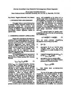
The m-dimensional vector ψh(t) describes the spiking history of the neuron up to time t according to a suitable parametrization. A simple parametrization is a spike histogram vector whose components contain the number of spikes in a set of preceding time windows. That is, the k-th component (ψh(t))k contains the number of spikes in the time window (t − ∆k+1, t − ∆k] with ∆ 0 < ∆1 < < ∆ m . The linear weights wh can then be fit empirically to model the specific dynamic properties of the neuron such as its refractory period or bursting behavior. The encoding scheme is illustrated in Figure 1. Analogous to the spike feedback just described, the encoding can readily be extended to the population case, if the vector ψh(t) for each neuron not only describes its own spiking history, but includes the spiking history of all other neurons as well. Taken together, the log-likelihood of observing the spike times {t ij } for a population of i = 1,…,N neurons is given by
({ }
)
T
( )
log p t ij | w is , w ih = ∑ log λ i t ij − ∫ λ i (s)ds
First, the stimulus is filtered with a linear filter ws which is referred to as the receptive field of the neuron. Subsequently, the pointwise monotonic nonlinearity f transforms the real-valued output of the linear filtering into a non-negative instantaneous firing rate. If the current stimulus has a strong overlap with the receptive
Frontiers in Computational Neuroscience
)
log p {t j } | w s , s(t ) = ∑ log λ(t j ) − ∫ λ(τ)dτ
www.frontiersin.org
i, j
((
= ∑ log f s t i, j
T
(
i j
0
)
( )
w is + ψ h t ij
)
w ih
− ∫ f s(τ) w is + ψ h (τ) w ih dτ.
)
(4)
0
May 2010 | Volume 4 | Article 12 | 2
Gerwinn et al.
Bayesian inference for GLMs
Figure 1 | Illustration of the generative encoding model associated with a GLM: the stimulus s(t) as well as the spiking history ψh(t) are filtered with their corresponding receptive fields ws and wh. A nonlinearity f is applied to the sum of the outputs to produce an instantaneous rate, which then is used to generate new spikes.
Although the likelihood factorizes over different neurons i, this does not imply that the neurons fire independently. In fact, every neuron can affect any other neuron i via the spiking history term ψh(t). Thus, by fitting the weighting term w ih to the data we can also infer effective couplings between the neurons. In order to evaluate Eq. 4 we have to calculate the integral ∫T0 f (s(τ) w is + ψ h (τ) w ih )dτ numerically. In terms of computation time, this easily becomes a dominating factor when the recording time T is large. Many artificial stimuli used for probing sensory neurons such as white noise can be described as piecewise constant functions. For example, the stimulus used for the retinal ganglion cells in Section “Population of Retinal Ganglion Cells” had a refresh rate of 180 Hz. In this case, the stimulus s(t) only changes at particular points in time. Further, if we use the spike histogram vector mentioned above to describe the spiking history of the neurons, then also ψh(τ) is a piecewise constant function. Thus, we can find time points τ1,…,τz between which neither the stimulus nor the vector describing the spiking history changes. We call the τi “discretization-points”. Also in cases in which the features are not piecewise constant such a discretization can be approximately obtained in a data-dependent manner, which we show in Section “Data-Dependent Discretization of the Time-Axis”. By decomposing the integral over (0, T) into a sum of integrals over the intervals [τk, τk+1) within which the integrand stays constant, the log-likelihood can be simplified to:
(
)
((
log p {t ij } | w is , w ih = ∑ log f s t ij i, j
)
( )
w is + ψ h t ij
(
w ih
) )
− ∑ ( τ k +1 − τ k ) f s(τ k ) w is + ψ h (τ k ) w ih (5) k ,i
Note that ψh(τk) and ψs(τk) are constant, since the features do not change in the interval [τk, τk+1). Extending the computational power of GLMs
To increase the flexibility of a GLM, several extensions are possible. For example, one can add hidden variables (Kulkarni and Paninski, 2007; Nykamp, 2008) or weaken the Poisson assump-
Frontiers in Computational Neuroscience
tion to a more general renewal process (Pillow, 2009). By adding only a few extra parameters to the model these extensions can be very effective in increasing the computational power of the neural response model. The downside of this approach is that most of these extensions do not yield a log-concave and hence unimodal posterior anymore. Another option for increasing the flexibility of the GLM which preserves the desirable property of concave log-posterior is to add more and more linearly independent parameters for the description of the stimulus and spike history that are promising candidates for improving the prediction of spike generation. For example, in addition to the original stimulus components s(t)i we can also include their quadratic interactions s(t)is(t)j. In this way, we can obtain an estimate of the computations of nonlinear neurons such as complex cells. This is similar to the spike-triggered covariance method (Van Steveninck and Bialek, 1988; Rieke et al., 1997; Rust et al., 2005; Pillow and Simoncelli, 2006) but more general, as we can still include the effect of the spike history. In principle, one can add arbitrary features to the description of both the stimulus as well as the spiking history. As a consequence, it is possible to approximate any arbitrary point process under mild regularity assumptions (see Daley and Vere-Jones, 2008). Like in standard least squares regression the actual merit of the Bayesian fitting procedure described in this paper is to have mechanisms for finding linear combinations of these features that provide a good description of the data. Therefore, it often makes sense to use a set of basis functions whose span defines the space of candidate functions (Pillow et al., 2005). We should choose a sufficiently rich ensemble of basis functions such that any plausible kind of stimulus or history dependence can be realized within this ensemble. We denote the feature space for the spiking history by ψh and the feature space for the stimulus by ψs. The concatenation of both feature vectors is denoted by ψs,h. Together we can write down the log-likelihood of observing a spike train {t ij } j , i :
(
)
( )
T
log p {t ij } | w s , w h = ∑ log λi t ij − ∑ ∫ λi (s )ds
www.frontiersin.org
i,j
i
0
(6)
May 2010 | Volume 4 | Article 12 | 3
Gerwinn et al.
Bayesian inference for GLMs
(
( )
= ∑ log f ψ h t ij i,j
T
( )
w ih + ψ s t ij
(
w is
)
)
− ∑ ∫ f ψ h (τ) w ih + ψ s (τ) w is dττ i
0
(7)
Data-dependent discretization of the time axis
If we choose the features ψh, ψs such that they do not change between distinct discretization-points τk, i.e., ψs,h is constant in the interval [τk, τk+1) the likelihood can be simplified to:
({ }
)
(
( )
log p t ij | w s , w h = ∑ log f ψ h t ij i, j
( )
w ih + ψ s t ij
(
w is
)
)
− ∑ ( τ k +1 − τ k ) f ψ h ( τ k ) w ih + ψ s ( τ k ) w is (8) i ,k
When approximating the features by describing the spike history dependence with a piecewise constant function, this yields a finite number of discretization-points in time between which, the resulting conditional rate, given the spiking history, does not change. In order to illustrate this process, consider the following simple scenario illustrated in Figure 2. Suppose there is only one neuron, which receives a constant input. Accordingly, the feature describing the stimulus is constant ψs(t) ≡ 1, which appear as the last entry in the combined feature vectors ψh,s(t) in the figure. The spiking history Ht up to time t is represented by two dimensions, which are approximated by piecewise constant functions, changing only at 2 and 10 ms. Note, that the time axis, labeled with time-parameter s in Figure 2 is pointing into the past and centered at the current time point t. As long as we did not observe a spike, the feature values of the two basis functions are zero, i.e., ψh(t)1 = ψh(t)2 = 0 for t