Abstract. We present a framework for efficient, accurate approximate. Bayesian inference in generalized linear models (GLMs), based on the ex- pectation ...
Bayesian Inference for Sparse Generalized Linear Models Matthias Seeger, Sebastian Gerwinn, and Matthias Bethge Max Planck Institute for Biological Cybernetics Spemannstr. 38, T¨ ubingen, Germany
Abstract. We present a framework for efficient, accurate approximate Bayesian inference in generalized linear models (GLMs), based on the expectation propagation (EP) technique. The parameters can be endowed with a factorizing prior distribution, encoding properties such as sparsity or non-negativity. The central role of posterior log-concavity in Bayesian GLMs is emphasized and related to stability issues in EP. In particular, we use our technique to infer the parameters of a point process model for neuronal spiking data from multiple electrodes, demonstrating significantly superior predictive performance when a sparsity assumption is enforced via a Laplace prior distribution.
1
Introduction
The framework of generalized linear models (GLM) [5] is a cornerstone of modern Statistics, offering unified estimation and prediction methods for a large number of models frequently used in Machine Learning. In a Bayesian generalized linear model (B-GLM), assumptions about the model parameters (sparsity, nonnegativity, etc) are encoded in a prior distribution. For example, it is common to use an overparameterized model with many features together with a sparsity prior. Only such features relevant for describing the data will end up having significant weight under the Bayesian posterior. Importantly, for the models of interest in this paper, inference does not require combinatorial computational efforts, but can be done even with a large number of parameters. Exact Bayesian inference is not analytically tractable in most B-GLMs. In this paper, we show how to employ the expectation propagation (EP) technique for approximate inference in GLMs with factorizing prior distributions. We focus on models with log-concave (therefore unimodal) posterior, for which a careful EP implementation is numerically robust and tends to convergence rapidly to an accurate posterior approximation. The code used in our experiments will be made publicly available. We apply our technique to a point process model for neuronal spiking data from multiple electrodes. Here, each neuron is assumed to receive causal input from an external stimulus and the spike history, represented by features in a GLM. In the presence of high-dimensional stimuli (such as images), with many neurons recorded at a reasonable time resolution, we end up with a lot of features,
but we can assume that the system can be described by a much smaller number of parameters. This calls for a sparsity prior, and we are able to confirm the importance of this prior assumption through our experiments, where our model achieves much better predictive performance with a Laplace sparsity prior than with a (traditionally favoured) Gaussian prior, especially for small to moderate sample sizes. Our model is inspired by [10], who identify commonly used spiking models as log-concave GLMs, but the Bayesian treatment as well as the usage of sparsity in this context is novel. The structure of the paper is as follows. In Section 2, we introduce and motivate the model class of B-GLMs. In Section 3, we show how the expectation propagation method can be applied to B-GLMs, motivating the central role of log-concavity in this context. Our multi-neuron spiking model is presented in Section 4, and experimental results are presented in Section 5. We close with a discussion in Section 6.
2
Bayesian Generalized Linear Models
The models we are interested in here are specified in terms of primary parameters w (or weights) and hyperparameters θ. If D denotes the set of observations, the likelihood is P (D|w), and the (Bayesian) prior distribution is P (w). We require that Y P (w|D) ∝ φj (uj ), uj = wT ψ j , (1) j
where P (w|D) ∝ P (D|w)P (w) is the (Bayesian) posterior. uj is a scalar-valued1 linear function of w, and the sites φj (·) are non-negative scalar functions. We require that all φj are log-concave, i.e. each − log φj is convex2 . The role of log-concavity is clarified shortly, see also Section 3. Note that our framework can be extended with no additional difficulties to models with an additional joint Gaussian factor N (w|µ0 , Σ 0 ) in (1). Here, Σ 0 need not be diagonal. Most Gaussian process models fall in our class, for example [9]. Perhaps the simplest B-GLM is the linear one, where the likelihood is Gaussian and given by factors φj (uj ) = N (yj |uj , σ 2 ), describing data D = {(ψ j , yj )}, yj ∈ R. Equivalently, yj = ψ Tj w + εj , where εj ∼ N (0, σ 2 ) is noise. If the linear model is used with a Gaussian prior on w, Bayesian inference can be done analytically, essentially by solving the normal equations. However, this convenient conjugate choice does not encode any strong assumptions about w and can severely underperform in situations where such assumptions are reasonable. What non-Gaussian priors can we use Q within our model class? We restrict ourselves to factorizing priors: P (w) = k P (wk ). Log-concave choices include the Laplace (or double exponential) P (wk ) ∝ e−ρk |wk | (sparsity); positive Gaussian P (wk ) ∝ N (wk |0, σk2 )I{wk >0} (non-negativity); or exponential distribution 1
2
Our framework applies just as well if the uj are low-dimensional vectors, but this is not in the scope of this paper. We allow for generalized convex functions, which may take the value +∞.
P (wk ) ∝ e−ρk wk I{wk >0} (sparsity and non-negativity). Furthermore, any product of log-concave functions is log-concave again.
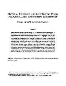
Gaussian
Laplace
Very Sparse
Fig. 1. Different prior distributions over coefficients of w.
In this paper, we are principally interested in the Laplace distribution as a sparsity prior. The linear model with this prior is the basis of the Lasso [19], extensively used in Machine Learning (under names such as L1 regularization, basis pursuit, and others). In the Lasso, we compute point estimates for the parameters, by maximizing the sum of the log likelihood and the log of the Laplace sparsity prior. The latter L1 regularizer tends to force coefficient estimates to zero exactly if they are not required. L1 penalization can be applied to nonlinear GLMs as well, resulting in a convex estimation problem, for which several algorithms have been proposed in Machine Learning. The Bayesian inference approach is quite different. Rather than just estimating a single parameter value, a posterior distribution over parameters is computed. More than a point estimate, we obtain credibility regions and information about parameter correlations from the posterior. Parameters are never forced exactly to zero under the posterior, since such a conclusion could not be justified from finite observations. The function of the Laplace sparsity prior in Bayesian inference is motivated in Figure 1. It leads to shrinkage of posterior mass towards coordinate axes (vertical in the figure), something a Gaussian prior does not do. On the other hand, the posterior remains log-concave, so that 0.4 all contours enclose convex sets. The stronger sparsity prior ∝ e−|aij | is not log-concave and induces a multimodal posterior, which can be very hard to approximate. Note that the role of the Laplace prior in our work here is not to provide feature selection or sparse estimation, but rather to improve our inference for an overparameterized model from limited data. Note that the method proposed here has been applied to Bayesian inference for the sparse linear model
underlying the Lasso in [16]. However, our application here requires a nonlinear model, since the data are event times rather than real-valued responses. Generalized linear models [5] extend the linear model to a range of different tasks beyond real-valued regression estimation, while maintaining desirable properties such as identifiability, efficient estimation, and simple asymptotics. All logconcave GLMs are of the form (1). The likelihood has exponential family form, in that P (D|w) = exp(φ(D)T g −l(g)−a(D)), where g = g(w) are the natural parameters, and l(g) is the log partition function, which is convex in g. If g is linear in w, then P (D|w) is log-concave in w, since − log P (D|w) = −φ(D)T w + l(g) up to a constant. Therefore, any log-concave factorizing prior on w induces a B-GLM. If g(w) is composed of a linear map and a nonlinear link function, log-concavity must be established separately. A concrete example of a B-GLM of this kind is given in Section 4. Importantly, the posteriors of B-GLMs are log-concave in w, therefore unimodal. This property is quite crucial to ensure that our approximate inference3 method is accurate and can be implemented in a numerically stable manner. Note that many models of general interest are not B-GLMs, such as mixture models, models with Student-t likelihoods. Many of the commonly used sparsity priors, such as “spike-and-slab” (mixture of narrow and wide Gaussian), Student-t, or ∝ exp(−ρ|wk |α ), α < 1 (see Figure 1 for α = 0.4), are not logconcave, and accurate approximate inference is in general a very hard problem. Furthermore, most approximate inference methods known today are numerically unstable when applied to such models. Several approximate inference methods for B-GLMs have been proposed. The MCMC technique of [11] could be applied, together with adaptive rejection sampling [3] for the likelihood factors. Our approach is significantly faster and more robust than MCMC (where convergence is very hard to assess). Sparse Bayesian Learning (SBL) [20] is the most well-known method for the sparse linear model. SBL is related to our EP variant in [16]. It has been combined with EP and applied to B-GLMs in [12]. The main technical difference to our proposal is that they use separate techniques to deal with likelihood sites (EP, moment matching) and prior sites (scale mixture decomposition of Student-t), while we employ EP for all sites. The EP update for Laplace prior sites is numerically challenging, and an equivalent direct EP variant for a non-log-concave Student-t prior (used in SBL) is likely to behave non-robustly (Malte Kuss, pers. comm.). The scale mixture treatment circumvents these numerical difficulties, and stronger sparsity Student-t priors can be used. On the other hand, our direct approach runs significantly faster on models of interest here, where there are many more likelihood than prior factors. The method of [12] is a double-loop algorithm, where EP is run to convergence on the likelihood sites after each update of the (prior) scale mixture parameters. Our method is also more transparent, not mixing two 3
Faced with non-log-concave models with multimodal posteriors, most approximate inference techniques somewhat break down, with the exception of MCMC techniques, which however typically become very inefficient in such situations.
different approximate inference principles4 . Finally, their method approximates a multimodal posterior with a single Gaussian in a variational lower-bound fashion (SBL can be interpreted in a variational way, see [22]), which is often quite loose. Typical robustness and “symmetry-breaking” problems in such methods are hidden in the optimization over the scale mixture (prior) parameters, which may be hard to solve properly. Even if their SBL approach is applied to a model with Laplace priors (by using the scale mixture decomposition of the Laplace, see [11]), the implications of posterior log-concavity for their method are less clear. Note that the Laplace approximation frequently used for approximate Bayesian inference cannot be applied directly to the sparse GLM, since the Hessian does not exist at the posterior mode. A double-loop method can be derived by applying the Laplace approximation to the likelihood only, this has been proposed in [20].
3
Expectation Propagation
Exact Bayesian inference is not analytically tractable for the application considered here, or for most B-GLMs in general. However, it can be approximated, and our approach is based on the expectation propagation (EP) method [7, 9]. EP results in a Gaussian approximation Q(w) to a posterior P (w|D) of the form (1). While the latter is not Gaussian, its log-concavity (and unimodality) motivates such an approximation. EP is used for a linear model (Gaussian likelihood) with Laplace prior in [16], and has been used for a range of models with Gaussian prior and log-concave likelihood [9], albeit not for point process data (as is done here; an application to discrete-state continuous-time Markov processes was given in [8]). In general, there has not been much work on approximate inference for nonlinear models with sparsity priors (an exception is [12]). The posterior P (w|D) in (1) is formally a product of J sites φj , normalized to integrate to one. Each site φj is either part of the likelihood P (D|w) or of the prior P (w). Let K be the number of variables: w ∈ RK . We use a factorizing Laplace prior on w, P (w) =
K Y
φk (wk ),
φk (wk ) ∝ e−ρ|wk | ,
ρ > 0,
(2)
k=1
whose sparsity-enducing role has been motivated above. The likelihood sites φj , j = K + 1, . . . , J in (1) are log-concave and will be specified further below for the model of interest. 4
These principles may in fact be based on qualitatively different divergence measures, noting that SBL has variational mean-field character [22], which uses a different divergence than EP [6]. Since these divergences focus on different aspects of approximation [6], mixing them is non-transparent and may lead to algorithmic problems such as slow convergence.
Q The EP posterior approximation of (1) has the form Q(w) ∝ j φ˜j (uj ), where φ˜j (uj ) = exp(bj uj − 12 πj u2j ) are site approximations of Gaussian form, the bj , πj are called site parameters. The log-concavity of the model implies that all πj ≥ 0. Some of them may be 0, as long as Q(w) is a (normalizable) Gaussian throughout. An EP update at j consists of computing the Gaussian cavity distribution Q\j ∝ Qφ˜−1 and the non-Gaussian tilted distribution Pˆ ∝ Q\j φj , j then updating bj , πj such that the new Q0 has the same mean and covariance as Pˆ (moment matching). This is iterated in some random ordering over the sites until convergence. Let Q(w) = N (w|h, Σ ). An EP update at site j leads to a rank-one update of Σ , featuring v j = Σ ψ j , and costs O(K 2 ). Details are given in the appendix. It is shown in [15] that for log-concave sites this update can always be done, and results in πj ≥ 0. In this case, EP updates can typically be done in a stable way, and empirically the method converges reliably and quickly. In contrast to this, EP tends to be very problematic to run on non-log-concave models. Full updates may not always be possible (for example resulting in negative variances), and damping techniques are typically required to attain convergence at all. Cases of EP divergence for multimodal posteriors have been reported [7]. EP updates often become inherently unstable operations in these cases5 . A good initialization of b, π depends on the concrete B-GLM. For our sparse spiking model (see Section 4), we start with b = 0, and πj = 0 for all likelihood sites, but πk = ρ2 /2 for prior sites, ensuring that φk (2) and φ˜k have the same first and second moments initially, k = 1, . . . , K. It is reported in [16] that in the presence of a factorizing Laplace prior, EP can behave extremely unstably if w is only weakly constrained by the likelihood. This happens in strongly underdetermined linear models (more variables than observations), but will typically not be the case in parametric B-GLMs. For example, in our spiking model application, we have many more likelihood sites than w components. In such cases, an initial EP update sweep over all likelihood sites is recommended, before any Laplace prior sites are updated. In an underdetermined case, the measures developed in [16] may have to be applied. The marginal likelihood P (D|θ) is the probability of the data, given model and hyperparameters θ, where primary parameters w have been integrated out. It is the normalization constant in (1). This quantity, also known as partition function or evidence, can be used to conduct Bayesian tests (via Bayes factors), or to adjust θ in a way robust to overfitting. EP comes with a marginal likelihood approximation, which in our case can be derived from [16, 15], together with its gradient w.r.t. θ. Details will be described in a longer version of this paper.
5
In this case, a multimodal posterior is approximated by a unimodal Gaussian, so that spontaneous “symmetry breaking” does occur. The outcome may then depend significantly on artificial choices such as site ordering for the updates, or numerical roundoff errors during the updates.
4
Sparse Feature Neuronal Spiking Model
An important approach to understanding neural systems is to build models in order to predict spike responses to natural stimuli [2]. Traditionally, single cell responses are characterized using spike-triggered averaging techniques6 , allowing for efficient estimation of the linear receptive field, a concise description of what the cell is most sensitive to. For example, a neuron in the early visual cortex may act as a detector of certain features such as edges or lighting/texture gradients of particular orientation in a small area of the visual field: its receptive field can be thought of as a localized, oriented filter, and only the appearance of the specific event will elicit a strong response. This notion can be grounded in a specific GLM: the linear-nonlinear cascade model [10]. Recent developments apply this formalism to multi-neuron responses [4, 10]. We present another important conceptual extension: rather than computing point estimates of model parameters only, we employ a full Bayesian inference scheme, allowing us to encode desirable properties via the prior. The resulting posterior gives quantitative answers about localization and dispersion of inferred model parameters, together with credibility intervals (“error bars”) describing the range of uncertainty in the parameters. Assessing uncertainty is essential in this application, since neural response models come with many parameters, and only a limited amount of data is available. We adopt linear-nonlinear-Poisson (LNP) cascade models [17], where spikes Di = {tj,i } of neuron i come from an inhomogeneous Poisson process, whose instantaneous firing rate λi (t) is a nonlinear function of the output of a linear filter. The filter coefficients are the primary parameters wi . λi (t) depends on both stimulus events as well as the spiking history of all neurons. There are stimulusneuron dependencies (normally described by the linear receptive field) as well as neuron-neuron dependencies: λi (t) may depend on spikes from D = ∪i Di , lying in [0, t). In summary, LNP models are obtained as λi (t) = λi (wTi ψ(t)), where ψ(t) does not depend on primary parameters: a linear filter is followed by a nonlinear transfer function λi , which feeds into an inhomogeneous Poisson process. According to general point process theory [18], the negative log likelihood for spike data D is Z X X − log λi (wTi ψ(tj,i )) + λi (wTi ψ(t)) dt . i
j
It has been shown in [10] that the likelihood is log-concave in wi if λi (·) is convex and log-concave. The model we consider here is a generalization of a Poisson Network [13], and a special LNP model. For a sequence of changepoints 0 = t˜0 < t˜1 < · · · < t˜j < . . . , we assume that ψ(t) is constant in each [t˜j−1 , t˜j ), attaining the value ψ j there. The semantics of changepoints are given below, here we note that all spikes 6
Statistics are obtained by averaging over a window [ti − ∆, ti ), ti a spike, characterizing effects which precede a spike emission [14].
(from all neurons) are changepoints, with ξj,i = 1 iff t˜j ∈ Di Q and ξj,i = 0 otherwise. Under this assumption, the likelihood is P (D|{wi }) = i Li (wi ), where each Li (wi ) has the form (1), with φj,i (uj,i ) = λi (uj,i )ξj,i exp(−τj λi (uj,i )), τj = t˜j − t˜j−1 . Importantly, while we require that all rates λi (t) are piecewise constant, we do not restrict ourselves to a uniform quantization of the time axis. The changepoint spacing is far from uniform, but rather tracks current spiking activity and stimulus quantization. A simple transfer function is λi (u) = eu , giving rise to a log-linear point process model. Another option is λi (u) = eu I{u