Beating the 'world champion' Evolutionary Algorithm via REVAC Tuning

Beating the ‘world champion’ Evolutionary Algorithm via REVAC Tuning S.K. Smit, and A.E. Eiben

Abstract— We present a case study demonstrating that using the REVAC parameter tuning method we can greatly improve the ‘world champion’ EA (the winner of the CEC2005 competition) with little effort. For ‘normal’ EAs the margins for possible improvements are likely much bigger. Thus, the main message of this paper is that using REVAC great performance improvements are possible for many EAs at moderate costs. Our experiments also disclose the existence of ‘specialized generalists’, that is, EAs that are generally good on a set of test problems, but only w.r.t. one performance measure and not along another one. This shows that the notion of robust parameters is questionable and the issue requires further research. Finally, the results raise the question what the outcome of the CEC-2005 competition would have been, if all of EAs had been tuned by REVAC, but without further research it remains an open question whether we crowned the wrong king.

I. BACKGROUND AND O BJECTIVES Finding appropriate parameter values for evolutionary algorithms (EA) is one of the persisting grand challenges of the evolutionary computing (EC) field. As explained by Eiben et al. in [7] this challenge can be addressed before the run of the given EA (parameter tuning) or during the run (parameter control). In this paper we focus on parameter tuning, that is, we are seeking good parameter values off-line and use these values for the whole EA run. In today’s practice, this tuning problem is usually ‘solved’ by conventions (mutation rate should be low), ad hoc choices (why not use uniform crossover), and experimental comparisons on a limited scale (testing combinations of three different crossover rates and three different mutation rates). Until recently, there were not many workable alternatives. However, by the developments over last couple of years now there are a number of tuning methods and corresponding software packages that enable EA practitioners to perform tuning without much effort. In particular, REVAC [16], [15], [18] and SPOT [3], [5], [4] are well developed and documented. Using algorithmic parameter tuners for EAs offers benefits on different time scales. The immediate benefits are obtained by the improved EA performance. Here the gains can be substantial, while the costs are low. In particular, the tuned EA can greatly outperform the EA based on usual parameter values, while the costs of a tuning session are by all means acceptable, typically in the range of hours. This makes algorithmic parameter tuners interesting for practitioners as well as EC scientists engaged in a performance-based competition (implicitly over a sequence of publications, or explicitly within a programming contest). The long term promise of Vrije Universiteit Amsterdam, The Netherlands, {sksmit, gusz}@cs.vu.nl

good and cheap tuning methods come from the accumulated information about the relationship between parameter values and EA performance. For instance, we might learn that parameter x has almost no impact on performance, that parameter x and y have a strong correlation, or that a certain EA will work better if we turn a constant c in its code into a variable v and tune it. Over the years, such information can be generalized into new insights and knowledge about EA behavior, leading to a deeper understanding of evolutionary computing in general. The main objective of this paper is to demonstrate the fist type of benefit. (Clearly, this also contributes to the long term benefits for the whole field by obtaining and publishing information about parameter values and EA performance.) To this end, we carry out an experimental comparison by the usual EC template: “Our EA beats your EA on an interesting set of test functions”, where the only difference between “our EA” and “your EA” is that “our EA” is simply “your EA” with tuned parameter values. To make the demonstration convincing we use an EA that has proved to be very good, hence hard to improve. To find such an EA we turn to the CEC-2005 contest on real valued function optimization, take the overall winner (G-CMA-ES) and try to improve its performance over the whole test suite by tuning it with REVAC. II. PARAMETERS , T UNERS , AND U TILITY L ANDSCAPES To obtain a detailed view on parameter tuning we distinguish three layers: the application layer, the algorithm layer, and the design or tuning layer, see Figure 1.

Fig. 1.

The three main layers in the hierarchy of parameter tuning.

As this figure indicates, the whole scheme can be divided into two optimization problems. The lower part of this threetier hierarchy consists of a problem on the application layer (e.g., the traveling salesman problem) and an EA (e.g., a genetic algorithm) on the algorithm layer trying to find an

TABLE I Method at work Search space Quality Assessment

problem solving evolutionary algorithm solution vectors fitness evaluation

parameter tuning tuning procedure parameter vectors utility testing

Utility Function Evolutionary Algorithm Test Problem(s)

optimal solution for this problem. Simply put, the EA is iteratively generating candidate solutions (e.g., permutations of city names) seeking one with maximal quality. The upper part of the hierarchy contains a tuning method that is trying to find optimal parameter values for the EA on the algorithm layer. Similarly to the lower part, the tuning method is iteratively generating parameter vectors seeking one with maximal quality, where the quality of a given parameter vector is based on the performance of the EA using the values of it. To avoid confusion we use distinct terms to designate the quality function of these optimization problems. Conform the usual EC terminology we use the term fitness for the quality of candidate solutions on the lower level, and the term utility to denote the quality of parameter vectors. Table I provides a quick overview of the related vocabulary. Using this nomenclature we can define the utility landscape as an abstract landscape where the locations are the parameter vectors of an EA and the height reflects utility, based on any appropriate notion of EA performance. It is obvious that fitness landscapes –commonly used in EC– have a lot in common with utility landscapes as introduced here. To be specific, in both cases we have a search space (candidate solutions vs. parameter vectors), a quality measure (fitness vs. utility) that is conceptualized as ‘height’, and a method to assess the quality of a point in the search space (evaluation vs. testing). Finally, we have a search method (an evolutionary algorithm vs. a tuning procedure) that is seeking for a point with maximum height. III. T UNING DEPENDENCIES As explained in the previous section, tuners are in essence heuristic optimizers of utility landscapes. By the very nature of the problem, the optimal solution depends on the test problem(s) to be solved, the evolutionary algorithm to be tuned, and the actual definition of utility. In practice, the tuner will find a set of very good solutions, i.e., parameter vectors for the EA to be tuned, that may or may not be optimal. This is shown in Figure 2. Given a tuner and a particular EA, the set of good parameter vectors for this EA will depend on • The notion of utility. • The test suite. It is important to note that the notion of utility is application dependent. In general, there are two ‘atomic’ performance measures for EAs: one regarding solution quality and one regarding algorithm speed. The most common measures in evolutionary computing reflecting these aspects are Mean Best Fitness (MBF) and Average number of Evaluations to Solution (AES) [9, Chapter 14]. Success Rate (SR) –a

Tuner

Set of good parameter values

Fig. 2. The theoretical optimum of a tuning problem depends on the problem(s) to be solved, the EA used, and the utility function. Adding the tuner to the equation we obtain this picture showing how a set of good parameter values obtained through tuning depends on four factors.

measure derived from a given target quality and the observed quality– is used very often too. In any particular case, one may tune on either of these performance measures, or a combination of them. Such combinations can be simply linear, using some kind of weighted average of MBF, AES, and SR1 . Additionally, one may define specific formulas to aggregate and combine information on EA runs. Our present study is based on three different performance measures, MBF, SR, and Rank, where Rank is an example of a special aggregation mechanism, as used in the CEC-2005 challenge [10]. The exact details will be given in Section V The second factor determining the set of good parameter values is the test suite. In simplest case, the utility of a parameter vector #» p is the performance of the EA using the values of #» p on a given test function F . Tuning an EA (by whichever performance metric) on one single function delivers a specialist, that is, an EA that is very good in solving that problem with no claims or indications regarding its performance on other problems. This can be a satisfactory result if one is only interested in solving that given problem. However, algorithm designers in general, and evolutionary computing experts in particular, are often interested in so called “robust parameter settings”, that is, in parameter values that work well on many problems. To this end, test suites consisting of many test functions are used to test and evaluate algorithms. For instance, a specific set {F1 , . . . , Fn } is used to support claims that the given algorithm is good on a “wide range of problems”. Tuning an EA (by whichever utility function) on a set of test functions delivers a generalist, that is, an EA that is very good in solving various problems. Obviously, a true generalist would perform well on all possible test functions. However, this is impossible by the no-free-lunch theorem [20]. Therefore, the quest for generalist EAs is practically limited to less general claims that still raise serious methodology issues as discussed in [8]. Technically, tuning an EA on collection of functions {F1 , . . . , Fn } means that the utility is not a single number, but a vector of utilities corresponding to each of the test functions. Hence, finding a good generalist is a multi-objective problem, for which each test-function is one objective. The 1 This option causes a problem of merging different measures and scales, but these issues are out of the scope of this paper.

current parameter tuning algorithms can only deal with tuning problems for which the utilities can be compared directly, therefore a method is needed to aggregate the utilityvectors into one scalar number. The need for such a higher level utility function is not limited to parameter tuning alone. While most recent publications, researchers present their algorithms based on a set of problems, a strict comparison function is not required. By showing the raw data and leaving the interpretation up to the reader, an aggregation can be avoided. However, in competitions, such as the one at the CEC-2005, there is the specific need for an aggregation method just as for parameter tuning. In this study, we restrict ourselves to simply averaging the utilities to obtain a single number, which can be compared easily. Finally, let us remark that utility and test function definitions have very interesting interactions that can lead to unexpected effects on the outcome of the tuning session, that is, the preferred parameter vectors. To illustrate this, let us assume a test suite containing easy and hard problems and let us decide to seek parameter vectors with equally good performance on each of the given test functions, i.e., using equal weights balancing the results on F1 , . . . , Fn . Assume furthermore that we use MBF as utility measure and that it is defined in such a way that it shows the mean error at termination. (This will be the case if all test functions are non-negative and have an optimum of zero.) Under these circumstances, we will obtain parameter vectors that are specialized in solving the hard problems in the test suite. This is caused by the fact that the range of MBF values on easy problems is much smaller, say from 10−5 to 10−6 , than the range on hard problems, say from 10−2 to 10−3 . Hence, improving the utility on an easy problem by a factor 10 is less beneficial than improving it on a hard problem. Consequently, even though we gave all test functions the same weight, the EA after tuning will be biased towards a high performance on the hard test problems. IV. S YSTEM D ESCRIPTION In this section, we give a general description of the components that instantiate the three layers as introduced in section II. A. Application Layer: CEC-2005 Test-suite We have chosen the 25 benchmark functions provided by Suganthan et al. [19] for the CEC 2005 Special Session on Real-Parameter Optimization. The 25 functions are supposed to cover a whole range of different problems without favoring certain types of algorithms. Functions F1 to F5 of the benchmark are unimodal (U) and F6 to F12 are basic multimodal. Functions F13 and F14 are expanded multimodal and F15 to F25 are hybrid multimodal test functions that are constructed by combining multiple standard test functions. In order to prevent exploitation of problem characteristics as symmetry, all problems are shifted and many of them are rotated. F4 and F17 are distorted by the addition of white noise. The CEC-2005 test-suite specifies that algorithms are allowed for 106 fitness evaluations per problem. Furthermore,

TABLE II T WO VIEWS ON A TABLE OF PARAMETER VECTORS . x ¯1 .. . x ¯n .. . x ¯m

D(x1 ) {x11

D(xi ) x1i

··· ···

D(xk ) x1k }

{xn 1

··· ··· .. . ···

xn i

xn k}

{xm 1

···

xm i

··· .. . ···

xm k }

Utility y1 .. . yn .. . m y

for each function a success-threshold is defined. If the best found fitness value is below this threshold, then it is regarded as ‘successful’. For comparison purposes, we have scaled F6 to F16 and F17 to F25 in such a way that all functions have a success-threshold of 10−6 . B. Algorithm Layer: G-CMA-ES As explained in the introduction, we deliberately use an EA that is hard to improve, thus making the task to our tuner more challenging. Our choice is the overall winner of the CEC-2005 contest, the so-called G-CMA-ES, a variant of the the CMA-ES from Hansen [2]. The CMA-ES is an ES that adapts the full covariance matrix of a normal search (mutation) distribution [11], [12], [13]. Compared to many other EAs, an important property of the CMA-ES is its invariance against linear transformations of the search space. For the details of this ES we refer to [10], here we only discuss the general principle and those aspects that play a role in our tuning exercise. In essence, the G-CMA-ES is a regular ES using µ parent vectors, λ offspring vectors, and self-adaptive mutation stepsizes (σ’s). The variables µ and λ are the usual parameters of this EA. Additionally, σ’s must be given an initial value before a run. The default population size prescribed for the CMA-ES grows logarithmically with the dimension of the search space (D) through the formula λ = 4 + 3 log2 (D). On multi-modal functions the optimal population size λ can be considerably greater than the default population size [10]. Furthermore, the value of µ is related to λ by the equation µ = λ2 . The other relevant feature of the CMA-ES is its restart policy. The definition of the algorithm includes a list of stopping criteria, and whenever one of these stopping criteria is met, an independent restart is launched with the population size increased by a factor of d = 2. Hansen and Auger [2] report that values between 1.5 and 5 could be reasonable for the increasing factor d. For the purposes of our present investigations only one of these stopping criteria is relevant: Stop if the range of the best objective function values of the recent generations is below a certain threshold e. C. Design Layer: REVAC On the design layer, REVAC [14] is used for tuning the parameters of the G-CMA-ES. For a good understanding of the method it is helpful to distinguish two views on a given set of parameter vectors as shown in Table II. Taking a horizontal view on the table, a row is a vector of k

parameter values and we can see the table as a list of vectors (first column), together with the utility of each vector (last column), defined through the performance of the EA in question. However, taking a vertical view on the table, the ith column in the inner box shows m values from the domain of parameter i and this can be seen as a distribution over the range of that parameter. To understand how REVAC is generating parameter vectors we can take the horizontal view. From this perspective, REVAC can be described as an evolutionary algorithm working on a population of m parameter vectors. This population is updated by selecting parent vectors, which are then recombined and mutated to produce one child vector that is then inserted into the population. The exact details are as follows. •

•

•

•

•

Parent selection is deterministic in REVAC as the n vectors of the population that have the highest measured utility are selected to become the parents of the new child vector. Recombination is performed by a multi-parent crossover operator, uniform scanning [6]. In general, this operator can be applied to any number of parent vectors and the ith value in the child hc1 , . . . , ck i is selected from the ithe values, x1i , . . . , xni , of the parents uniform randomly. Here we create one child from the selected n parents. Mutation, applied to the offspring created by recombination, is rather complicated. It works independently on each parameter i in two steps. First, a mutation interval [xia , xib ] is calculated, then a random value is chosen uniformly from this interval to be the mutated value. To define the mutation interval for mutating a given ci all values x1i , . . . , xni for this parameter in the selected n parents are also taken into account. After sorting them in increasing order, the begin point of the mutation interval can be specified as the h-th lower neighbor of ci , while the end point of the interval is the h-th upper neighbor of ci . The mutated value c0i is drawn from this interval with a uniform distribution and the child will be composed of these mutated values hc01 , . . . , c0k i. (As there are no neighbors beyond the upper and lower limits of the domain, we extend it by mirroring the parent values as well as the mutated values at the limits.) Survivor selection is also deterministic in REVAC as the newly generated child always replaces the vector in the population with the worst performance. Evaluation The utility of the newly generated child is estimated by running the EA to be tuned with the values it contains.

V. E XPERIMENTAL S ETUP Here we complement the general description of the system components from the previous section by defining their parameters and other specific details as used in our experiments.

A. G-CMA-ES Unlike most evolutionary algorithms, the G-CMA-ES does not have generally recommended default values for its parameters. To be precise, its default parameter values are not defined as fixed numbers, but as a function of other parameters and/or problem characteristics, [10]. This may suggest fewer parameters, however, most of these functions still contain “magic constants” like the 2 in µ = λ2 or the 3 in λ = 4 + 3 · log2 (n). To be able to tune the population size, the offspring size, and the initial mutation stepsize, we decided to tune these “magic constants”. In this way, we combine the knowledge of the authors about parameter interactions enclosed in these formulas, and the power of REVAC to tune parameters. The parameter-functions and the constants tuned are summarized in Tables III and IV. This setup requires k = 5 parameters to be tuned. The G-CMAES is implemented in Java by Hansen and integrated into the MOBAT toolkit. 2 TABLE III PARAMETERS , DEFINING FORMULAS , AND MAGIC CONSTANTS OF THE G-CMA-ES Parameter

Symb.

Offspring size Population size Step size Population multiplication Stop Crit. theshold

λ µ σ d e

Defining formula λ = 4 + a · log2 (n) µ = λb σ = c · (Lu − Lb )

Magic const. a b c

TABLE IV S ETUP OF THE G-CMA-ES. T HIS TABLE SUMMARIZES THE “ MAGIC ” CONSTANTS INTRODUCED IN TABLE III. To be tuned a b c d e Termination

Value-range [1, 10] [1, 5] [0.02, 10] [1, 4] [0, 0.001]

Recommended Value 3 2 0.5 2 10−12 10.000 evals

B. REVAC On the design layer, REVAC [14] is used for tuning the parameters of the Evolutionary Algorithm. REVAC itself has some parameters too, which need to be specified. The values of the REVAC parameters used in these experiments are shown in Table V. It can be argued that by using REVAC, the number of parameters that need to be specified is hardly reduced. Instead of five G-CMA-ES parameters, one now needs to specify four REVAC parameters while the runtime is 5000 times as long. However, one has to bear in mind that the goal of parameter tuning is not to find the best possible solution for the problem at the application layer, but the best 2 Based on our verification experiments, we can conclude that the implementation in Java slightly differs from the version implemented in Matlab

possible setup (parameter vector) for the algorithm. Once found, this setup can be reused in further runs and similar applications. TABLE V REVAC PARAMETERS Population Size Best Size Smoothing coefficient Repetitions per vector Maximum number of vectors tested

80 40 10 5 5000

C. Utility functions The CEC-2005 optimization contest crisply specifies the metrics used to compare the competing evolutionary algorithms. The two principal components of these metrics are the test suite and the EA performance measure. Furthermore, there are rules on technical details, for instance about the required precision when optimizing the given objective functions, the number of fitness evaluations EAs are allowed to do, or the number of independent runs with an EA to calculate its performance. In general, any experimental comparison between EAs is based on some metric X. Then it is a natural idea to use this metric X as utility function within the tuner to find an EA that scores well on X. In principle, this guarantees that (the parameters of) the EAs are optimized for the right objectives. Our present study follows this rationale, but makes a number of practical compromises that amount to using slightly modified version X 0 of the final comparison metric as utility function. The modifications are such that X 0 is in essence the same as X, but it can be calculated much faster. As for the test suite, the CEC-2005 rules specify that a contestant EA is to be tested on each of the 25 problems (equally weighted), and is allowed to use D · 104 fitness evaluations per run per problem, where D is the dimensionality of the given problem. In order to reduce the time used for tuning, we decided that REVAC calculates utility values based on D · 103 fitness evaluations only. This reduces the duration of the tuning sessions at the cost of the quality of information used to guide the tuning algorithm. Although it is likely that the best possible parameter vector with D · 103 evaluations differs from the best with D · 104 evaluations, our results indicate that the best parameter vector found also performs well using D · 104 evaluations without the corresponding tuning costs. As for the EA performance measures, the official CEC2005 list contains three of them, • MBF, • SR, • Rank (defined below), and the rules prescribe that the performance of each EA is to be calculated based on 25 independent runs. In this study all three performance measures are used to form utility functions and we tune the G-CMA-ES for each of these independently. This implies that we perform three complete

tuning sessions such that REVAC is using either of these performance measures to calculate the utility of parameter vectors. For each of these utility functions it holds that u(~ p) of a parameter vector p~ is calculated by running the G-CMA-ES 5 times independently on the whole test suite with the parameter values in p~. This represents a second modification of the final comparison metrics meant to deliver computationally cheaper utility functions. Once again, we deliberately trade quality of information for execution speed, and the results show that this is not harmful. To coop with the two notions of algorithm quality (parameter quality) we introduce the term estimated utility and verified utility. Estimated utility stands for the one used during the tuning session, i.e., during a REVAC run. In general, this is the X 0 in the first paragraph of this section; here this is based on D · 103 fitness evaluations and 5 repetitions. By verified utility we mean the one used for reporting the final outcomes. In general, this is the X in the paragraph above, and it corresponds to the ultimate comparison metric behind the given experimental study. Here we use the official CEC-2005 definitions, based on D · 104 fitness evaluations and 25 repetitions. To complete this section EA performance measures need to be specified. MBF and SR are commonly used ones, therefore we omit their definitions. Rank, however, is not that well known. Conceptually, ranks is a lexicographic ordering based on SR (primary measure) and MBF (secondary measure) such that the best parameter vector gets rank 1. An important difference between MBF and SR on the one hand, and Rank on the other hand is that SR and MBF can be calculated for any parameter vector v in isolation, while Rank is a relative measure showing how good v is within a set of vectors V . Technically, given a set V of parameter vectors, the rank R(v) of any v ∈ V is calculated in two different ways, depending on its SR value: • if SR(v) > 0, then R(v) equals its SR-based rank in {u ∈ V : SR(u) > 0} • if SR(v) = 0, then R(v) equals its MBF-based rank in {u ∈ V : SR(u) = 0} plus |{u ∈ V : SR(u) > 0}| This definition allows us to calculate rank R for any set of parameter vectors. During a tuning session with REVAC, the set V is changing over time and at any time t it is the set of all parameter vectors that have been generated and tested till that time. D. Software and Hardware Description The complete experiment is defined in MOBAT[17] (MetaHeuristic Optimizer Benchmark and Analysis Toolbox), a toolbox for defining, tuning and evaluating Evolutionary Algorithms on a distributed system. The default package of MOBAT contains all the components for composing the evolutionary algorithm used in these experiments, the testfunctions and REVAC. MOBAT is open source and freely available via SourceForge.net. The experiments are ran using the distributed-features of MOBAT on a 2.93 GHz Intel Core 2 Duo and a 2.8 GHz Dual Quad Core Xeon machine, and

took 12 days to finish all together, costing roughly 4 days per performance measure. VI. R ESULTS The results from the experiments can be investigated from two different viewpoints, namely the performance of the best parameter vectors (one for each utility function), and the values of the best parameter vectors themselves (again, one for each utility function).

mendation and in Table IX we compare our best EA with the overall winner of that contest. TABLE IX C OMPARING THE ORIGINAL AND THE REVAC- TUNED VERSIONS OF THE G-CMA-ES. (F OR MBF AND R ANK , LOWER IS BETTER .) EA REVAC-tuned ES CEC-2005 winner

Performance over the whole test suite by Mean Best Fitness Success-rate Rank 2.5e-3 29.9% 1.48 7.7e-3 29.9% 2.80

A. Performance In this section we present the outcomes of our experiments by showing the verified utilities of the three best parameter vectors (one for each utility function) in Table VI,VII and VIII, together with the results obtained by using the recommended parameter values in the G-CMA-ES. From these data it is immediately clear that the performance measure used for tuning highly influences the utilities. Comparing the outcomes discloses that for each of our three measures, the best parameter vector is the one that is tuned on that specific measure. While this is not surprising per se, it is worth mentioning as it confirms that REVAC is capable of tuning an EA for a specific user preference, e.g., MBF, SR, or Rank. It also shows that the recommended parameters that are used in the G-CMA-ES are very good for solving the ‘easy’ functions, but on ‘hard’ functions they perform far worse. From Table VI we can observe how the choice for Mean Best Fitness as performance measure has influenced the results. The best found vector does not perform well on the ‘easy’ functions, hardly reaching values below 10−6 . However, on the ‘hard’ functions, especially F15 it outperforms all other vectors. As predicted in section III, during tuning it was mainly aimed at improving the MBF on functions with high objective values, rather than generally improving the MBF. This effect is clearly visible in table VII. Furthermore, on hardly any of the problems, the best found fitness dropped below the success-threshold. The opposite is true for the parameter vector found by using success-rate as performance measure. On most of the easy functions, it outperformed the other vectors, and was often able to get the perfect score of 25 successes out of 25 runs. However, on the ‘hard’ functions it performed much worse. Table VIII shows this ‘all or nothing’ behavior in which it either is the best, or the worst of the three tuned vectors. The recommended parameters perform reasonably well on the success-rate, which was one of the main criteria in the evaluation of the CEC-2005 competition. The parameter vector found by tuning on the rank shows the most constant behavior. It performs well on the easy functions, and not very bad on the hard functions. What is also clear from table VIII is that the small increase in MBF on the hard functions was enough to compensate for the loss in performance on the ‘easy’ functions. This shows the effect of using the ranks, rather than the raw performance value. Keeping the rules of the CEC-2005 contest in mind we take the Rank-optimal parameter vector as our final recom-

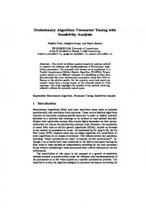
B. Best Parameter Values The results in the previous section clearly show that the performance measure used withing the tuner highly influences the results on the 25 test problems. The vector tuned on MBF is focused on a few ‘hard’ problems, while the one tuned on success-rate is mainly focused on the easy problems. The question rises which parameters are responsible for these different behaviors. In table X we display the three best parameter vectors (one for each performance measure) with their verified utility. The difference between the recommended parameters and the tuned values is clear. The e-value for the three tuned vectors values are up to 105 times as big, resulting in much more restarts without losing to much precision. However, to indicate the differences between the three tuned vectors figure 3 is much more informative. Figure 3 shows the top 1% of all generated vectors in each run, based on the corresponding utility function. The gray area shows the .05 and .95 quantile of these best performing parameter values. From these figures it is immediately clear that e and c highly influence the MBF. As could be expected, e needs to be large for an optimal performance based on MBF. This ensures that on ‘hard’ problems as many repetitions as possible are executed. Secondly, these figure 3 and table X also show the importance of the stepsize c, namely only very small values lead to the best MBF performance. Although hard to see, c and e are also the most influential parameters when tuning on success-rate and rank. The parameters that are tuned for success-rate are mainly focused at solving unimodal problems. Therefore, the values for stepsize c and stop-condition e are quite low in order to gradually climb towards to the success-threshold without restarts. However, compared to the recommended settings still much more restarts are executed. For rank based performance, both e and c are somewhat larger. This ensures a good fitness on ‘hard’ problems, due to a larger number op repetitions and a broader search. Based on these results, we can conclude that there is no such thing as “robust parameter values”, because the good parameter values depend strongly on the performance measure, even for generalist EAs optimized for a large collection of problems. VII. C ONCLUSIONS AND O UTLOOK Perhaps the most catchy aspect of this paper is the evidence that using REVAC we could improve the ‘world

TABLE X B EST PARAMETERS F OUND BY REVAC

a b c d e

Default value 3 2 0.5 2 10−12

Performance measure used for tuning Mean Best Fitness Success-rate Rank 4.82 4.93 3.61 2.34 1.31 1.14 0.14 0.55 0.81 1.13 2.37 1.20 4.0 · 10−4 1.8 · 10−6 2.8 · 10−5

champion’ EA in just a few days, spent on tuning its parameters. While this can be seen as a nice result itself, it is the far reaching implications of this case study that form the main message of this paper. Namely, this exercise demonstrates the ease of improving EA performance by using an automated tuning method. In other words, we have shown that the costs of tuning with our technology are by all means acceptable. Our case study also gives a hint about the possible gains. Considering that the ‘world champion’ EA must have been carefully designed and optimized approximating its best possible performance, the room for possible further improvements could not be very large. Yet, we succeeded in improving it easily. For ‘normal’ EAs that are not pushed to their limits yet, the margins for possible improvements are expectedly much much bigger and all our experience with REVAC indicates that it is possible to realize these improvements. To formulate it simply, the main message of this paper is that using REVAC great performance improvements are possible for many EAs at acceptable costs. Our results also indicate that one has to be careful with claims about robust parameters. In particular, we found that using different EA performance measures for tuning can lead to different optimal parameter vectors. In other words, REVAC has disclosed the existence of ‘specialized generalists’, that is, EAs that are generalists in the sense of performing well on a large set of test problems (rather than on one problem only), but are specialists in the sense that they perform well only along one performance measure and not along another one. This shows that the very notion of robust parameters is questionable. The easy fix for this problem is to extend the definition of robustness to two dimensions and consider good performance over multiple problems and over multiple performance measures separately. However, we feel that it is more advisable to dedicate further research efforts to this to sort out all related aspects. Finally, the question arises what the outcome of the CEC2005 competition would have been, if all of the participants had tuned their algorithm by REVAC. Definitely, some algorithms would have benefited more from tuning than others. The results, hence the final rankings, would have been most likely different, but without further research it remains an open question whether we crowned the wrong king. R EFERENCES [1] Proceedings of the 2005 IEEE Congress on Evolutionary Computation, Edinburgh, UK, 2-5 September 2005. IEEE Press.

[2] A. Auger and N. Hansen. A restart CMA evolution strategy with increasing population size. In Proceedings of the 2005 IEEE Congress on Evolutionary Computation IEEE Congress on Evolutionary Computation [1], pages 1769–1776. [3] T. Bartz-Beielstein, C.W.G. Lasarczyk, and M. Preuss. Sequential parameter optimization. In Proceedings of the 2005 IEEE Congress on Evolutionary Computation IEEE Congress on Evolutionary Computation [1], pages 773–780 Vol.1. [4] T. Bartz-Beielstein, K.E. Parsopoulos, and M.N. Vrahatis. Analysis of Particle Swarm Optimization Using Computational Statistics. In Chalkis, editor, Proceedings of the International Conference of Numerical Analysis and Applied Mathematics (ICNAAM 2004), pages 34–37, 2004. [5] Thomas Bartz-Beielstein and Sandor Markon. Tuning search algorithms for real-world applications: A regression tree based approach. Technical Report of the Collaborative Research Centre 531 Computational Intelligence CI-172/04, University of Dortmund, March 2004. [6] A.E. Eiben and Th. B¨ack. An empirical investigation of multiparent recombination operators in evolution strategies. Evolutionary Computation, 5(3):347–365, 1997. [7] A.E. Eiben, R. Hinterding, and Z. Michalewicz. Parameter Control in Evolutionary Algorithms. IEEE Transactions on Evolutionary Computation, 3(2):124–141, 1999. [8] A.E. Eiben and M. Jelasity. A Critical Note on Experimental Research Methodology in EC. In Proceedings of the 2002 IEEE Congress on Evolutionary Computation (CEC 2002), pages 582–587. IEEE Press, 2002. [9] A.E. Eiben and J.E. Smith. Introduction to Evolutionary Computing. Springer, 2003. [10] N. Hansen and S. Kern. Evaluating the CMA evolution strategy on multimodal test functions. In Xin Yao, Edmund K. Burke, Jos´e Antonio Lozano, Jim Smith, Juan J. Merelo Guerv´os, John A. Bullinaria, Jonathan E. Rowe, Peter Ti˜no, Ata Kab´an, and Hans-Paul Schwefel, editors, PPSN, volume 3242 of Lecture Notes in Computer Science, pages 282–291. Springer, 2004. [11] N. Hansen, S.D. Muller, and P. Koumoutsakos. Reducing the time complexity of the derandomized evolution strategy with covariance matrix adaptation (CMA-ES). Evolutionary Computation, 11(1):1–18, 2003. [12] N. Hansen and A. Ostermeier. Adapting arbitrary normal mutation distributions in evolution strategies: The covariance matrix adaptation. pages 312–317, 1996. [13] N. Hansen and A. Ostermeier. Completely derandomized selfadaptation in evolution strategies. Evolutionary Computation, 9(2):159–195, 2001. [14] V. Nannen and A. E. Eiben. Relevance Estimation and Value Calibration of Evolutionary Algorithm Parameters. In Manuela M. Veloso, editor, Proceedings of the 20th International Joint Conference on Artificial Intelligence (IJCAI), pages 1034–1039, 2007. [15] V. Nannen and A.E. Eiben. A method for parameter calibration and relevance estimation in evolutionary algorithms. In M. Keijzer, editor, Proceedings of the Genetic and Evolutionary Computation Conference (GECCO-2006), pages 183–190. Morgan Kaufmann, San Francisco, 2006. [16] V. Nannen and A.E. Eiben. Relevance estimation and value calibration of evolutionary algorithm parameters. In Proceedings of the International Joint Conference on Atrificial Intelligence (IJCAI’07), pages 975–980. International Joint Conferences on Artificial Intelligence, AAAI Press, 2007. [17] S.K. Smit. MOBAT. http://mobat.sourceforge.net, 2009. [18] S.K. Smit and A.E. Eiben. Comparing parameter tuning methods for evolutionary algorithms. In Proceedings of the 2009 IEEE Congress on Evolutionary Computation, pages 399–406, Trondheim, May 18-21 2009. IEEE Press. [19] P.N. Suganthan, N. Hansen, J.J. Liang, K.Deb, Y.-P. Chen, A. Auger, and S. Tiwari. Problem definitions and evaluation criteria for the cec 2005 special session on real-parameter optimization. Technical report, Nanyang Technological University, 2005. [20] David H. Wolpert and William G. Macready. No free lunch theorems for optimization. IEEE Transaction on Evolutionary Computation, 1(1):67–82, 1997.

TABLE VI R ESULTS USING M EAN B EST F ITNESS AS PERFORMANCE MEASURE Parameter Vector Recommended Parameters Best found using mean best fitness Best found using success-rate Best found using rank Parameter Vector Default Parameters Best found using mean best fitness Best found using success-rate Best found using rank

AVG 7.7e-3 2.0e-3 3.0e-3 2.5e-3 F13 8.9e-5 6.3e-5 6.0e-5 6.0e-5

F1 4.5e-15 5.6e-7 4.7e-9 1.1e-7 F14 3.4e-4 3.3e-4 1.0e-4 1.5e-4

F2 2.2e-15 6.7e-7 5.1e-9 1.2e-7 F15 3.4e-2 5.5e-3 2.8e-2 1.5e-2

F3 0.0e-15 5.0e-7 6.2e-9 1.0e-7 F16 1.1e-2 6.5e-3 7.8e-3 7.4e-3

F4 4.5e-15 7.9e-7 6.8e-9 2.0e-7 F17 1.0e-3 1.0e-3 9.7e-4 1.0e-3

F5 2.4e-11 1.1e-5 2.3e-7 9.3e-7 F18 8.4e-3 3.0e-3 3.2e-3 3.0e-3

F6 4.7e-5 4.9e-4 5.8e-8 1.3e-6 F19 7.6e-3 3.0e-3 3.2e-3 3.0e-3

F7 4.7e-7 8.2e-5 1.1e-7 2.6e-7 F20 8.2e-3 3.0e-3 3.8e-3 3.0e-3

F8 2.0e-3 2.0e-3 2.0e-3 2.0e-3 F21 9.0e-3 3.0e-3 4.9e-3 5.0e-3

F9 9.7e-4 1.7e-4 1.1e-4 1.3e-4 F22 7.7e-3 7.3e-3 7.2e-3 7.2e-3

F10 7.9e-4 2.0e-4 1.3e-4 1.2e-4 F23 8.3e-3 8.7e-3 8.0e-3 8.1e-3

F11 1.3e-4 9.9e-5 6.1e-7 6.4e-6 F24 2.3e-3 2.0e-3 2.0e-3 2.0e-3

F12 8.6e-2 4.6e-6 4.0e-5 2.6e-7 F25 4.0e-3 4.0e-3 4.0e-3 4.0e-3

TABLE VII R ESULTS USING S UCCESS - RATE AS PERFORMANCE MEASURE ( ONLY SOLVED FUNCTIONS ARE SHOWN )

Parameter Vector Recommended Parameters Best found by mean best fitness Best found by success-rate Best found by rank

Problems Solved 9 5 11 11

SR 29.9 % 1.4 % 37.7 % 29.9 %

F1 25 25 25 25

F2 25 22 25 25

F3 25 25 25 25

F4 25 19 25 25

F5 25 0 25 16

F6 22 0 25 11

F7 24 0 25 25

F9 0 0 8 4

F10 0 0 4 4

F11 7 0 25 0

F12 9 2 24 25

F16 0 0 0 2

TABLE VIII R ESULTS USING THE RANK AS PERFORMANCE MEASURE Parameter Vector Recommended Parameters Best found using mean best fitness Best found using success-rate Best found using rank Parameter Vector Recommended Parameters Best found using mean best fitness Best found using success-rate Best found using rank

AVG 2.80 2.44 1.60 1.48 F13 4 3 1 1

F1 1 1 1 1 F14 4 3 1 2

a

b

c

(a) Tuned on Mean Best Fitness Fig. 3.

F3 1 1 1 1 F16 4 2 3 1

F4 1 4 1 1 F17 2 2 1 2

F5 1 4 1 3 F18 4 1 3 1

F6 2 4 1 3 F19 4 1 3 1

F7 3 4 1 1 F20 4 1 3 1

F8 1 1 1 1 F21 4 1 3 2

F9 4 3 1 2 F22 4 3 1 1

a

e

d

F2 1 4 1 1 F15 4 1 3 2

F11 2 4 1 3 F24 4 1 1 1

F12 3 4 2 1 F25 1 1 1 1

a

e

b

d

F10 4 3 1 1 F23 3 4 1 2

c

(b) Tuned on Success Rate

e

b

d

c

(c) Tuned on Rank

The good parameter ranges when using the three different performance measures. The parameter ranges from Table IV are scaled to [0, r]