Bi-level Multi-objective Programming Problem with

International Journal of Computer Applications (0975 – 8887) Volume 30– No.10, September 2011

Bi-level Multi-objective Programming Problem with Fuzzy Parameters Surapati Pramanik

Partha Pratim Dey

Department of Mathematics, Nandalal Ghosh B.T. College, Panpur, P.O.- Narayanpur, District – North 24 Parganas, Pin code-743126, West Bengal, India

Patipukur Pallisree Vidyapith, 1, Pallisree Colony, Patipukur, Kolkata-700048, West Bengal, India

ABSTRACT This paper deals with fuzzy goal programming approach to bilevel multi-objective programming problem with fuzzy parameters. In the proposed approach, the tolerance membership functions for the fuzzily described objective functions are defined by determining individual optimal solution of the objective functions of each of the decision makers. Since the objectives are potentially conflicting in general, possible relaxations of both level decisions are considered by providing preference bounds on the decision variables for avoiding decision deadlock. Then fuzzy goal programming technique is used for achieving highest degree of each of the membership goals by minimizing negative deviational variables. An algorithm is presented with termination criteria. An illustrative numerical example is provided to demonstrate the efficiency of the proposed approach.

General Terms Bi-level multi-objective programming.

Keywords Bi-level programming, Deviational variables, Fuzzy goal programming, Fuzzy parameters, Tolerance membership functions.

1. INTRODUCTION Bi-level multi-objective programming problem (BLMOPP), an apparatus for modeling decentralized decisions, consists of the objectives of the first level decision maker (FLDM) at its first level and that of the objectives of the second level decision maker (SLDM) at the second level. The execution of decision is sequential, from first level to second level; each decision maker (DM) independently controls only a set of decision variables and is interested in optimizing his/her net benefits over a common feasible region. Although each DM independently tries to optimize his/her own objective function, the decision may be affected by the actions and reactions of the SLDM due to the dissatisfaction with the decision. During the last three decades, bi-level programming problem (BLPP) [1, 2] as well as multi-level programming problem (MLPP) [3, 4, 5] in general for hierarchical decentralized planning problems have been deeply studied and many methodologies have been developed to solve them. Sinha [6] studied multi-level programming technique based on fuzzy mathematical programming. Pramanik and Roy [7] proposed a solution methodology based on fuzzy goal programming (FGP)

for solving MLPP. Sakawa et al. [8] developed interactive fuzzy programming for MLPP with fuzzy parameters in 2000. Shi and Xia [9] studied two-person bi-level multi-objective decision making and an interactive algorithm to solve non-linear bi-level multi-objective decision-making problem. Abo-Sinha [10] discussed multi-objective optimization for solving non-linear multi-objective bi-level programming problem in fuzzy environment. Abo-Sinha and Baky [11] presented balance space approach for nonlinear multi-objective bi-level programming problem. Baky [12] studied FGP algorithm for solving decentralized bi-level multi-objective programming problems. Zhang et al. [13] presented an algorithm to fuzzy linear multiobjective bi-level programming problems by using  -cut method. Gao et al. [14] studied fuzzy linear BLMOPP based on  -cut and goal programming. Pramanik and Roy [15] studied FGP approach to multi-objective transportation problem with fuzzy parameters. Pramanik and Roy [16] also discussed priority based FGP approach to multi-objective transportation problem with fuzzy parameters. Recently, Pramanik [17] modified FGP model due to Pramanik and Roy [15, 16] and applied it to BLPP with fuzzy parameters. In this paper, we extend the concept of BLPP due to Pramanik [17] for BLMOPP. In the model formulation of the problem, we first formulate membership functions by determining individual best and worst solution of the objective functions for both the DMs for a prescribe value of . Since the objectives of FLDM and SLDM are conflicting in nature, cooperation between both level DMs is necessary to reach a compromise optimal solution. We assume that the SLDM first provides his/her decision by providing fixed preference upper and lower bounds on the decision variables under his/her control. Considering the fixed preference bounds of SLDM, the FLDM also presents his/her preference bounds on the decision variables under his/her control to avoid decision-deadlock [18]. Then, FGP approach [17] is used to solve the problem by minimizing negative deviational variables. The rest of the paper is organized as follows. Section 2 provides some basic definitions. Section 3 presents the formulation of BLMOPP. Section 4 discusses fuzzy programming model of BLMOPP having fuzzy parameters. In subsection 4.1, characterization of membership functions of BLMOPP with fuzzy parameter is presented. Subsection 4.2 provides FGP model of BLMOPP. Section 5 presents FGP algorithm to BLMOPP. In section 6, we solve an illustrative numerical example. Finally, section 7 provides the concluding remarks.

13

International Journal of Computer Applications (0975 – 8887) Volume 30– No.10, September 2011

2. PRELIMINARIES

X1 = {X11, X12, …, X 1N1 }T : decision vector under the control

Some basic definitions: ~ ~ Definition 2.1 A fuzzy set F in X is characterized by F = { x,

of FLDM

 ~F (x)  x X }, where  ~F (x): X  [0, 1] is called the

X 2 = {X21, X22, …, X 2 N 2 }T : decision vector under the control

 ~F (x) is the degree of

membership function of X and ~ membership to which x F .



~

~ ~ Definition 2.2 Union of two fuzzy sets F1 and F2 with respective

membership functions  ~F (x),  ~F (x) is characterized by a 1 2 ~ fuzzy set F3 whose membership function is defined by

~ ij

~ ij

~ ij

~ ij

~ ~ Definition 2.3 Intersection of two fuzzy sets F1 and F2 with

respective membership functions  ~F (x),  ~F (x) is defined by 1 2 ~ a fuzzy set F3 whose membership function is defined 1

2

~ Definition 2.4 The  -cut of a fuzzy set F of X is a non-fuzzy ~ set denoted by  F and defined by a subset of all elements x

(6)

~

~

Here, A1 is M  N1 and A 2 is M  N2 matrix, B is the M ~ ij  ~ ij ~ ij ~ ij  component column vector. C k =  Ck1, Ck 2 ,..., CkNk  (k = 1, 2)    

~

by  ~F  ~F (x) =  ~F (x) = min [  ~F (x),  ~F (x)], x X . 3

~ ij

~ ij

~

2

~ ij

(5)

= C11 X11  C12 X12  ...  C1N1 X1N1  C21 X 21  C22 X 22 

2

1

~ ij

Zij X = C1 X1  C2 X 2 , (i = 1, 2), (j = 1, 2, …, Mi)

...  C2 N 2 X 2 N 2 , (i = 1, 2), (j = 1, 2, …, Mi)

 ~F  ~F (x) =  ~F3 (x) = max [  ~F1 (x),  ~F2 (x)], x X . 1

of SLDM.



~



are constants. Z1 X , Z2 X are linear and bounded with fuzzy coefficients. For simplicity, let us denote the system constraints (3) and (4) as S ( ).

X so that their membership functions exceed or equal to a real ~ number   [0, 1], i.e.  F = x :  ~F (x)  ,  [0,1], x   .

4. FORMULATION OF FUZZY PROGRAMMING MODEL OF BLMOPP HAVING FUZZY PARAMETERS

3. FORMULATION OF BLMOPP

The optimal solution of FLDM and SLDM when determined in isolation would be considered as the aspiration level of each of the respective fuzzy objective goal. Then, for a prescribed value





Consider a BLMOPP of minimization-type objective functions at each level. Suppose that DMi denotes the DM at the i-th level (i = 1, 2) who controls the decision vector X i = (X i1 , X i 2 , …, X iNi ) ∈R

Ni

(i = 1, 2) where, X = X1  X 2 and N = N1+N2.

~

~

N2  M  N1 Zi ( X1 , X 2 )= Zi ( X ):  R  R   R i (i = 1, 2) are the   vector of objective functions of the DM i (i = 1, 2). Mathematically, the problem can be formulated as:

~



of , minimization-type objective function, ij  (i = 1, 2), (j = 1, 2, …, Mi) can be replaced by the lower bound of its  -cut 



ij

L

ij

~ ~  ~    ij   =  (C1 ) L X1   (C 2 ) L X 2 (i = 1, 2), (j = 1, 2, …,     Mi) (7)

i.e.

Similarly, for a prescribed value of  , maximization-type ~

objective function, Zij (X) (i =1, 2), (j = 1, 2, …, Mi) can be replaced by the upper bound of its  -cut i.e.

(First level) ~

~

~

~

Min Z1 (X) = Min ( Z11(X), Z12(X),..., Z1M1 (X) )

(1)

X1

X1

(Second level) ~

~

~



ij

U

ij

~ ~  ~    ij   =  (C1 ) U X1  (C2 ) U X 2 (i = 1, 2), (j = 1, 2, …,     Mi) (8) For the inequality constraints

~

Min Z2 (X) = Min ( Z21(X), Z22(X),..., Z2M 2 (X) )

(2)

X2

X2



N ~  AijX j j1

~

 Bi (i = 1, 2, …, m1)

(9)

subject to ~

~

A1 X1  A2 X2 , , B

X1  0 , X 2  0 .

and

~

(3) (4)

N ~  AijX j j1

~

 Bi (i = m1+1, …, m2)

(10)

can be rewritten by the following constraints as:

14

International Journal of Computer Applications (0975 – 8887) Volume 30– No.10, September 2011

N  j1



and

U

~   Aij  X j     

N  j1





L

~   Bi  (i = 1, 2, …, m1)    

L

~   Aij  X j     



(11)

L Let,  ( Z1Bj )L (j = 1, 2, .., M1) and  ( ZB 2 j ) (j = 1, 2, …, M2) be

U

~   Bi  (i = m1+1, …, m2)    

(12)

the individual optimal decision of the FLDM and SLDM respectively when calculated in isolation. Here,

For the fuzzy equality constraints N ~  AijX j j1

4.1 Characterization of membership functions of BLMOPP with fuzzy parameters



~ 1j

~

XS

XS

~

 Bi (i = m2+1, …, M)

(13)

(j = 1, 2, .., M1)

(21) ~ 2j

~



and

L

~   Aij  X j     

N  j1





~   Bi     

U

~   Aij  X j     



(14)

L

~   Bi  (i = m2+1, …, M)    

(15)

(j = 1, 2, …, M2) (22) If the individual optimal solutions of the objective functions of DMs are same, then compromise optimal solution is automatically reached. However, this situation rarely occurs due to the conflicting nature of the objectives. Then the fuzzy objective goals of the FLDM and SLDM appear as: 

For proof of equivalency of (13) with (14) and (15), see Lee and Li [19].

~

( Z1 j (X))L 

~



~

( Z2 j (X))L 

1

(16)

L ( ZB 2 j ) (j = 1, 2, …, M2)

( Z1Wj ) U



~

   ~  ~ ~  L  L  L Min  ( Z 21(X)) , ( Z 22 (X)) ,..., ( Z 2M (X))  2 2     

(24)



~ 1j



~ 1j

= Max ( Z1 j (X) = Max ( (C1 ) X1  (C2 ) U X 2 ) , U

U

XS

XS

(25) ~ 2j

~

~ 2j

( Z2Wj ) U = Max  ( Z2 j (X) U = Max ( (C1 ) U X1  (C2 ) U X 2 ) XS

2

XS

(j =1, 2, …, M2) (17)

(26)

Here,  ( Z1Bj )L ,  ( Z1Wj ) U (j = 1, 2, …, M1) are best and worst solutions respectively for FLDM. L  W U Similarly,  ( ZB 2 j ) and ( Z2 j ) (j = 1, 2, .., M2) are best and

subject to







~

N  j1



~

(23)

(j = 1, 2, .., M1)

Min  (  2 (X)) L =



( Z1Bj )L , (j = 1, 2, …, M1)

To formulate membership functions for the minimization type objective functions we define:

the following problem: Min  ( 1 (X)) L =

N  j1



~

Therefore, for a prescribed value of  , the problem reduces to

   ~  ~ ~  L  L  L Min  ( Z11(X)) , ( Z12 (X)) ,..., ( Z1M (X))  1 1     

XS

XS

U

(i = m2+1, …, M)

~ 2j

 L L  L  L and  ( ZB 2 j ) = Min ( Z2 j (X) = Min ( (C1 ) X1  (C2 ) X 2 )

can be replaced by two equivalent constraints N  j1

~ 1j

( Z1Bj )L = Min  ( Z1 j (X)L = Min ( (C1 )L X1  (C2 )L X 2 )

U

 ~   Aij  X j      L

 ~   Aij  X j     





X j ≥0 (j = 1, 2).

worst solutions respectively for SLDM.

L

~  Bi  (i = 1, 2, …, m1, m2+1, …, M)    

(18)

Then, the resulting membership functions for FLDM can be formulated as:

(19)

1j ( (1j()L ) 

U

~  Bi  (i = m1+1, …, m2, m2+1, …, M)    

(20)

For a prescribed value of  , the fuzzy BLMOPP reduces to deterministic BLMOPP which can be solved by using modified FGP model presented by Pramanik [17].

              U  ,

 W U  L  if 1j  ≥ 1j 0,    W U    L  B L  L  W  1j 1j , if 1j ≤ 1j  ≤ 1j   U  B L W  1j - 1j   L  B L if 1j  ≤ 1j 1,

        

(j = 1, 2, …, M1)

    

  

(27)

15

International Journal of Computer Applications (0975 – 8887) Volume 30– No.10, September 2011 Similarly, the resulting membership functions for SLDM can be formulated as:

5. FGP ALGORITHM TO BLMOPP WITH FUZZY PARAMETERS

2 j ( (2j()L ) 

By the following steps, we present the proposed FGP algorithm for solving BLMOPP with fuzzy parameters as follows:

        U        

 W U  L  if  2j  ≥  2j 0,    W U -   L  L  L  W  2j 2j , if  B   2j ≤  2j  ≤  2j U  B L W   2j -  2j  L  L  if  2j  ≤  B 1, 2j

        

    

(j = 1, 2, .., M2)

Step 1: For specified value of , to formulate the membership functions corresponding to the objective functions of both level DMs, the upper and lower bounds of their  - cuts are defined. Similarly, for inequality constraints, the upper bound and lower bound of their  - cuts are defined.

  

(28)

Suppose that  2 j and  2 j (j = 1, 2, …, N2) are the fixed upper and lower bounds on the decision variables provided by SLDM such that  2 j ≤ X2j ≤  2 j (j = 1, 2, …, N2). Let 1 j and 1 j (j = 1, 2, …, N1) be the upper and lower bounds on the decision variables provided by FLDM by considering the preference bounds of SLDM. It is to be noted that the FLDM may vary his/her preference bounds for overall benefit of the organization [18].

4.2 Formulation of FGP Model of BLMOPP The proposed FGP formulation for solving BLMOPP can be presented as: M1

M2

Minimize  = ∑ w 1j D1j  ∑ w -2j D -2j j 1

j 1

(29)

subject to = 1, (j = 1, 2, …, M1) 1j  (1j())L + D1j

(30)

2 j  (2j())L + D -2j = 1, (j = 1, 2, ..., M2)

(31)

N





j 1 

U

 ~   A ij  X j     L







L

~  i  , (i = 1, 2, …, m1, m2+1, …, M) (32)     U

 ~  ~  A ij  X j   i  ,(i = m1+1, …, m2, m2+1, …, M)(33)     j 1     (34) 1 j ≤ X1j ≤ 1 j , (j = 1, 2, …, N1) N



 2 j ≤ X2j ≤  2 j , (j = 1, 2, …, N2)

(35)

D1j  0 (j = 1, 2, …, M1), D -2j  0 (j = 1, 2, ..., M2),

(36)

X1  0 , X 2  0.

(37)

The numerical weights corresponding to negative deviational variables are determined as [15]. By solving FGP model (29), if FLDM and SLDM are satisfied with this solution, then satisficing solution is reached.

Step 2: Determine the individual maximum and minimum values for the upper and lower  - cuts of the objective functions for both level DMs subject to the system constraints. Step 3: Determine the weight wij  1/[ (ZijW )U  (ZijB )L ] (i = 1, 2), (j = 1, 2, …, Mi ). Step 4: Formulate the membership function ij (  (ij () L ) , (i = 1, 2), (j = 1, 2, …, Mi ). Step 5: Let, the preference bounds of SLDM on the decision variables be  2 j ≤ X2j ≤  2 j (j = 1, 2, …, N2). Then, the FLDM provides his/her preference bounds on the decision variables such that 1 j ≤ X1j ≤ 1 j (j = 1, 2, …, N1). Step 6: Formulate the FGP model (29) and solve the problem. If the solution is acceptable to both the DMs, then compromise optimal solution is reached. Otherwise, the FLDM provides another set of preference upper and lower bounds considering fixed preference bounds of SLDM. Step 7: Termination criteria: The family of distance functions [20] is defined as: 1/ p

 k  D p w, t  =   w pt 1  d t p   t 1    Here, d t (t =1, 2, …, k) denotes the degrees of closeness of the preferred compromise solution to the optimal solution vector with respect to t-th objective function. w = (w1, w2, …, wk) is the vector of attribute attention levels U  B L w t . We assume that w t  1/[ (ZW t )  ( Zt ) ] . The power p denotes the distance parameter 1 ≦ p ≦  . 1/ 2

 k  For p = 2, D 2 w, t  =   w 2t 1  d t 2   t 1   

For maximization problem, d t is defined by d t = (the preferred compromise solution)/ (the individual best solution). For minimization problem, d t is defined by d t = (the individual best solution)/ (the preferred compromise solution). The solution, for which D 2 w, t  will be minimum would be the most satisfying solution for FLDM and SLDM. Step 8: End.

16

International Journal of Computer Applications (0975 – 8887) Volume 30– No.10, September 2011

Consider the following BLMOPP with fuzzy parameters ~ ~ ~ ~   Z11(X)  (X1  3 X 2  2 X3  3 X 4 ),  ~  ~ ~ ~ ~ Min  Z12 (X)  (2 X1  9 X 2  3 X3  5 X 4 ),  (First level) X1 , X 2  ~ ~ ~ ~   Z13(X)  (3 X1  9 X 2  9 X3  X 4 )    ~ ~ ~ ~ ~   Z (X)  (6 X1  3 X 2  2 X3  2 X 4 ),  Min  ~ 21  (Second level) ~ ~ ~ ~ X1 , X 2   Z ( X )  ( 5 X  9 X  9 X  6 X ) 22 1 2 3 4   subject to

~

~

~

~

X1 + (3 -  ) X2 - X3 + X4  28 + 2 , X1, X2, X3, X4

Min

~



(Z11(X))L = X1 + 2.5 X2 + X3 + 2.5 X4,



(Z12(X))L = X1 + 8.5 X2 + 2.5 X3 + 4.5 X4,



(Z13(X))L = 2.5 X1 + 8.5 X2 + 8.5 X3 + X4,

X1 , X 2

Min X1 , X 2

Min X1 , X 2 ~

2 X1  4 X2  2 X3  2 X4  35 ,

Min



(Z21(X))L = 5.5 X1 + 2.5 X2 + X3 + X4,



(Z22(X))L = 4.5 X1 + 8.5 X2 – 8.5 X3 + 5.5 X4,

X3 ,X 4 ~

 0.

For,  = 0.5, the fuzzy BLMOPP reduces to deterministic BLMOPP as follows:

~

3 X1  X2  X3  3 X4  48 , ~

 37 - 2 ,

2  X1 + (3+  ) X2 + 2  X3 - 2  X4

6. NUMERICAL EXAMPLE

~

X1  2 X2  X3  X4  30 ,

Min X3 ,X 4

X1, X2, X3, X4 ≥ 0. subject to Here, all the fuzzy numbers are assumed to be triangular fuzzy numbers and are given as follows ~

~

~

~

~

2 = (0, 2, 3), 3 = (2, 3, 4), 4 = (3, 4, 5), 5 = (4, 5, 6), 6 = (5, 6, ~

~

~

~

7), 8 = (6, 8, 10), 9 = (8, 9, 10), 30 = (28, 30, 32), 35 = (33, 35, ~

2.5 X1 - X2 + X3 + 2.5 X4

 48.5,

 36,

X1 + 3.5 X2 + X3 - X4

X1 + 2.5 X2 - X3+ X4  29,

37), 48 = (45, 48, 49).

X1, X2, X3, X4  0.

By replacing the fuzzy coefficients by their  -cuts, the above problem can be written as

The individual best solutions subject to the system constraints

Min



X1 , X 2

Min



X1 , X 2

(Z11(X))L = X1 + (2+  ) X2 + (2  ) X3 + (2+  ) X4, (Z12(X))L = (2  ) X1 + (2+  ) X2 + (2+  ) X3 +

X1 , X 2

Min







L (ZB 21) = 29 at (0, 10.833, 0, 1.917), 10.833, 15.833, 17.5).



B L ( Z12 ) = 48.862 at



L (ZB 22 ) = 55.875 at (0,

W U ( Z11 ) = 111.048 at (0, 17.871, 0, 26.548),

271.371 at (0, 17.87, 0, 26.584),

(Z21(X))L = (5+  ) X1 + (2+  ) X2 + (2  ) X3 + (2  )

0),



(Z22(X)) = (4+  ) X1 + (8+  ) X2 - (8+  ) X3 + L

the

fuzzy

W U ( Z12 ) =

W U ( Z13 ) = 242.042 at (0,

W U ( Z21 ) = 126.705 at (21.102, 4.256, 0,

goals

appear

as



( Z11(X))L 

29,

~



( Z12(X))L  48.862, ~

(5+  ) X4,







W U ( Z22 ) = 297.919 at (0, 17.87, 0, 26.584).

Then, 



B L ( Z13 ) = 48.862 at (0, 3.31, 0, 20.724),



10.833, 15.583, 17.5),

X4,

Min

B L ( Z11 ) = 29 at (11.5, 7, 0, 0),

(20.724, 3.31, 0, 0),

are

(Z13(X))L = (2+  ) X1 + (8+  ) X2 + (8+  ) X3 + X4,

X3 ,X 4

X3 ,X 4



The individual worst solutions subject to the system constraints

(4+  ) X4,

Min

are

29,





( Z13(X))L  48.862, ~



( Z21(X))L  ~

( Z22(X))L  -55.875. ~

subject to (2+  ) X1 - X2 + X3 + (2+  ) X4

 49 - ,

Now, we construct the membership functions for both level DMs as follows:

17

International Journal of Computer Applications (0975 – 8887) Volume 30– No.10, September 2011

11 (Z11(X)) L =

111.048 (X1  2.5X 2  X 3  2.5X 4 ) , (111.048 29)

12 (Z12 (X)) L =

271.371 (X1  8.5 X 2  2.5 X 3  4.5 X 4 ) , (271.371 48.862)

297.919  (4.5X1  8.5X 2  8.5 X 3  5.5X 4 ) + d22 =1, (297.919 55.875) 2.5 X1 - X2 + X3 + 2.5 X4 X1 + 3.5 X2 + X3 - X4

242.042 (2.5X1  8.5X 2  8.5 X 3  X 4 ) , 13 (Z13(X)) L = (242.042 48.862)

 21 (Z21(X)) L =

126.705 (5.5 X1  2.5 X 2  X 3  X 4 ) , (126.705 29)

 22 (Z22 (X)) L =

297.919  (4.5X1  8.5X 2  8.5 X 3  5.5X 4 ) (297.919 55.875)

Let, the fixed preference bounds provided by the LLDM on the decision variables be 2



X3  15,

1  X4  17 Then the proposed FGP model for solving BLMOPP with fuzzy parameters is as follows: Min = (d11/ (111.048 - 29)) + (d12/ (271.371 – 48.862)) + (d13/ (242.042 – 48.862)) + (d21/ (126.705 - 29)) + (d22/ (297.919 – 55.875)), subject to

111.048 (X1  2.5X 2  X 3  2.5X 4 ) + d11 =1, (111.048 29) 271.371 (X1  8.5 X 2  2.5 X 3  4.5 X 4 ) + d12 =1, (271.371 48.862)

 48.5,

 36,

X1 + 2.5 X2 - X3+ X4  29, 2



X3  15,

1  X4  17, X1, X2, X3, X4

 0.

The results obtained by considering different preference bounds provided by FLDM are shown in the Table 1. Now from Table 1, we see that the minimum distance value is 0.01084. The optimal compromise solution of the problem is given by X1* = 10, X*2 = 7.5, X*3 = 2, X*4 = 2.5.The objective values are Z11 = 37, Z12 = 90, Z13 = 108.25, Z21 = 78.25, Z22 = 105.5. The corresponding membership values are 11 = 0.902, 12 = 0.815, 13 = 0.692,  21 = 0.496,  22 = 0.795.

Note: All solutions of the problem are obtained by Lingo, 6.0.

7. CONCLUSIONS In this paper, we have considered an alternative FGP approach to BLMOPP with fuzzy parameters. The proposed approach can be extended to optimization problems in different fields such as agriculture planning problems, decentralized planning problems and other multi-objective programming problems consisting fuzzily described different parameters. The proposed approach can also be extended to decentralized multi-objective as well as multi-level multi-objective programming problem with fuzzy parameters.

8. ACKNOWLEDGEMENTS 242.042 (2.5X1  8.5X 2  8.5 X 3  X 4 ) + d13 =1, (242.042 48.862)

The authors are very grateful to the anonymous referees for their valuable comments and necessary suggestions.

126.705 (5.5 X1  2.5 X 2  X 3  X 4 ) + d21 =1, (126.705 29)

18

International Journal of Computer Applications (0975 – 8887) Volume 30– No.10, September 2011  ij



ij L

1





O

ijW L



ij L

ijB U

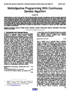
 ~   L Figure1. Membership function for objective function  (  ij ( ))  (i = 1, 2), (j = 1, 2, …, M i).     Table1. Comparison of optimal solutions based on distance function Serial No

Fixed preference bound of LLDM

preference bound of ULDM

Solution point

Objective values

Membership values

Distance values

1

2 ≤ x3 ≤ 15, 1 ≤ x4 ≤ 17

12 ≤ x1 ≤ 17, 6.5 ≤ x2≤ 18

12, 6.833, 2, 1.917

35.875, 83.707, 106.998, 87, 105.624

0.916, 0.843, 0.699, 0.406, 0.794

0.01095

2

-

11.5 ≤ x1 ≤ 16, 6.5 ≤ x2 ≤ 17.5

11.5, 7, 2, 2

36, 85, 107.25, 84.75, 105.25

0.915, 0.838, 0.698, 0.429, 0.796

0.01094

3

-

10.5 ≤ x1 ≤ 16, 6.5 ≤ x2 ≤ 17

10.5, 7.333, 2, 2.167

36.25, 87.582, 107.748, 80.25, 104.5

0.912, 0.826, 0.695, 0.475, 0.799

0.01091

4

-

10 ≤ x1 ≤ 17.5, 6.5 ≤ x2 ≤ 16.5

10, 7.5, 2, 2.5

37, 90, 108.25, 78.25, 105.5

0.902, 0.815, 0.692, 0.496, 0.795

0.01084

5

-

9 ≤ x1 ≤ 17, 6 ≤ x2 ≤ 16

9, 7.833, 2, 2.417

36.625, 91.457, 108.498, 73.5, 103.374

0.907, 0.808, 0.691, 0.544, 0.804

0.01085

6

-

9 ≤ x1 ≤ 17.5, 6 ≤ x2 ≤ 16

9, 7.833, 2, 2.241

36.185, 90.665, 108.322, 73.324, 102.406

0.912, 0.812, 0.692, 0.546, 0.808

0.01179

[3]

Lai, Y. J. 1996. Hierarchical Optimization: A satisfactory solution. Fuzzy Sets and Systems 77, 321 – 335.

[4]

Shih, H. S., Lai, Y. J., and Lee, E. S. 1996. Fuzzy approach for multi-level programming problems. Computers & Operations Research 23, 73 – 91.

[5]

Shih, H. S., and Lee, E. S. 2000. Compensatory fuzzy multiple level decision making. Fuzzy Sets and Systems 14, 71 – 87.

9. REFERENCES [1]

[2]

Candler, W., and Townsley, R. 1982. A linear bilevel programming problem. Computers & Operations Research 9, 59 - 76. Fortuny-Amat, J., and McCarl, B. 1981. A representation and economic interpretation of a twolevel programming problem. Journal of the Operational Research Society 32, 783 - 792.

19

International Journal of Computer Applications (0975 – 8887) Volume 30– No.10, September 2011

[14]

Gao, Y., Zhang, G., Ma, J., Lu, J. 2010. A  - cut and goal programming – based algorithm for fuzzy – linear multi-objective bilevel optimization. IEEE transactions on fuzzy system 18 (1), 01 - 13.

Pramanik, S., and Roy, T. K. 2007. Fuzzy goal programming approach to multilevel programming problems. European Journal of Operational Research 176 (2), 1151 - 1166.

[15]

Pramanik, S., and Roy, T. K. 2006. A fuzzy goal programming technique for solving multi-objective transportation problem. Tamsui Oxford Journal of Management Sciences 22 (1), 67 - 89.

Sakawa, M., Nishizaki, I., and Uemura, Y. 2000. Interactive fuzzy programming for multi-level linear programming problems with fuzzy parameters. Fuzzy Sets and Systems 109 (1), 03 – 19.

[16]

Shi, X., and Xia, H. 1997. Interactive multi-objective decision making. Journal of Operational Research Society 48, 943 - 949.

Pramanik, S., and Roy, T. K. 2008. Multiobjective transportation model based on priority based fuzzy goal programming. Journal of Transportation Systems Engineering and Information Technology 7 (3), 40 48.

[17]

Abo-Sinha, M. A. 2001. A bilevel non-linear multiobjective decision making under fuzziness. Operation Research Society of India (OPSEARCH) 38 (5), 484 - 495.

S. Pramanik, “Bilevel programming problem with fuzzy parameters: a fuzzy goal programming approach”, Journal of Applied Quantitative Methods, 2011, in press.

[18]

Abo-Sinha, M. A., and Baky, I. A. 2006. Interactive balance space approach for solving bilevel multiobjective programming problems. Advances in modeling and Analysis B 49 (3-4), 43 - 62.

Pramanik, S., and Dey, P. P. 2011. Bi-level linear fractional programming problem based on fuzzy goal programming approach. International Journal of Computer Applications 25 (11), 34-40.

[19]

Lee, E. S., and Li, R. J. 1993. Fuzzy multiple objective programming with pareto optimum. Fuzzy Sets and Systems 53, 275 – 288.

[20]

Zeleny, M. 1982 Multiple criteria decision making. McGraw-Hill, New York.

[6]

Sinha, S. 2003. Fuzzy programming approach to multi-level programming problems. Fuzzy Sets and Systems 136, 189 – 202.

[7]

[8]

[9]

[10]

[11]

[12]

[13]

Baky, I. A. 2009. Fuzzy goal programming algorithm for solving decentralized bi-level multi-objective programming problems. Fuzzy Sets Systems 160, 2701 - 2713. Zhang, G., Lu, J., and Dillon, T. 2007. Decentralized multi-objective bilevel decision making with fuzzy demand. Knowled – Based System 20 (5), 495 - 507.

20