Bias-corrected nonparametric correlograms for ... - UPCommons

ERAD 2010 - THE SIXTH EUROPEAN CONFERENCE ON RADAR IN METEOROLOGY AND HYDROLOGY

Bias-corrected nonparametric correlograms for geostatistical radar-raingauge combination Reinhard Schiemann1, Rebekka Erdin1, Marco Willi1, Christoph Frei1 Marc Berenguer2, Daniel Sempere-Torres2 1Federal Office of Meteorology and Climatology MeteoSwiss, Kraehbuehlstrasse 58, P.O. Box 514, 8044 Zurich, Switzerland, [email protected] 2Centro de Recerca Aplicada en Hidrometeorologia, Universitat Politècnica de Catalunya, C/Gran Capità, 2-4, Edifici NEXUS 102-106, 08034 Barcelona, Spain

Presenting author Christoph Frei

(Dated: 5 September 2010) 1.

Introduction

Geostatistical methods have been widely used for quantitative precipitation estimation (QPE) based on the combination of radar and raingauge observations. They are flexible and accurate and allow for radar-raingauge combination in real-time. Even within the area of geostatistical methods, however, a wide range of choices have to be made when planning for a particular application. These choices regard, for example, the actual combination method (e.g., kriging with external drift, cokriging), the kriging neighbourhood (global vs. local), the technique used to estimate the parameters of the geostatical model (e.g., least-squares, maximum-likelihood estimation), and the transformation of the precipitation variable. In addition to these issues, there are a number of options for modeling spatial dependencies in the precipitation data. Correlograms (variograms) for kriging are customarily one-dimensional, but two- or higher-dimensional correlation maps are also used and are one way of taking spatial anisotropy into account. Furthermore, correlograms can be parametric or nonparametric, they can be obtained from the radar or the raingauge data, and they can be estimated flexibly on a case-by-case basis or with data from a longer period of time. Recently, nonparametric correlograms based on spatially complete radar rainfall fields have been used in combining radar and raingauge data [1]. Here, we compare the estimation of nonparametric correlograms with the estimation of parametric semivariogram models conventionally used in geostatistical applications. We identify and explain a bias of the nonparametric correlograms towards too low ranges, and suggest a correction for this bias. 2.

Semivariogram estimation

The semivariogram of a spatial process Z is defined as (for greater detail see [2], whose notation we largely follow): (1)

γ (s i , s j ) = 12 Var(Z (si ) − Z (s j ))

For a 2nd order stationary process Z, this is equivalent to (2)

γ (s i − s j ) = 12 E((Z (s i ) − Z (s j )) 2 ) ; and

(3)

γ (si − s j ) = σ 2 (1 − ρ (s i − s j )) , where σ 2 = C (0) = Var(Z ) , and ρ (s i − s j )

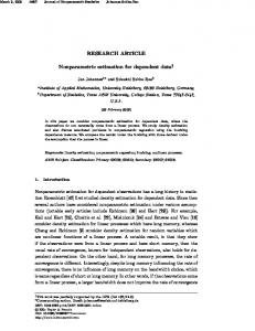
are the variance and the correlation function of the process Z, and E(·) denotes an expectation value. The widely-used Matheron-estimator for the semivariance reads (we denote estimators with a hat to distinguish them from theoretical quantities): Fig. 1. Semivariogram and correlogram estimation. (a) One-dimensional synthetic N ( s i −s j ) data sample, (b) semivariogram cloud, (c) N(si-sj) denotes the set of all pairs of observations at a given lag distance and empirical semivariogram and fitted parametric model, (d) theoretical and |N(si-sj)| is the number of such pairs. For complete radar grids of dimensions estimated correlograms. (4)

γˆ (s i − s j ) =

1 2 N (s i − s j )

∑ (Z (s ) − Z (s i

j

)) 2 , where

ERAD 2010 - THE SIXTH EUROPEAN CONFERENCE ON RADAR IN METEOROLOGY AND HYDROLOGY N1 · N2 ·… this number is equal to (N1-k) · (N2-l) ·…, where k, l, … are the components of the lag distance vector in units of the grid spacing. The customary procedure for estimating a semivariogram model is illustrated by means of synthetic data in Fig. 1a-c. Fig. 1a shows a single realization of a one-dimensional Gaussian random process with variance 1 and an exponential correlation function (the practical range, i.e. the lag at which the correlation decays to 0.05, equals 0.6 for this process). The sample semivariogram (or the so-called semivariogram cloud) is shown in Fig. 1b. It shows semivariogram ordinates for all pairs of observations. Since these values scatter substantially, it is customary to smooth the sample semivariogram by calculating the estimate (4) after pooling the semivariogram ordinates into a number of lag distance classes. This yields the so-called empirical semivariogram shown in Fig. 1c (open circles). Finally, a parametric model is fit to the empirical semivariogram. Here, a curve-fitting technique has been used to estimate an exponential semivariogram model (dashed line in Fig. 1c). Equation (3) yields the correlation function corresponding to the fitted semivariogram model (Fig. 1d, dashed line). The theoretical correlation function is shown by the solid black line in Fig. 1d. The difference between the estimated and the theoretical correlation is due to sampling variability and a bias of the estimator and will be discussed later. The use of a parametric model has a number of reasons. First, the parametric models are chosen such that they fulfill the property of positive definiteness. Correlation functions with this property can be used in geostatistical interpolation (kriging; see relevant texts such as [2] for details). Additionally, the parametrization further smoothes the empirical semivariogram and allows to estimate the correlation at unobserved lag distances. 3.

Estimation of nonparametric correlograms The nonparametric estimate of the correlation function is given by (5)

ρˆ (s i − s j ) = Z =

1 N

∑

N

i =1

1 N

 Z (s ) − Z  i ∑  ˆ N ( si −s j )  C ( 0)

Z (si ) and Cˆ (0) =

1 N

 Z (s ) − Z j   Cˆ (0) 

∑

N i =1

  , where  

( Z (si ) − Z ) 2

are the sample (also called plug-in) mean and variance, and N is the number of observations (e.g., radar grid points). This estimator can be conveniently computed in terms of the discrete Fourier transform (DFT). In fact, the Wiener–Khinchin theorem affirms that the magnitude of the DFT of the standardized observations is the spectral representation of the (auto-)correlation estimate computed in (5). Thus, (5) can be obtained rather simply by computing the DFT, multiplying with the complex conjugate and computing the inverse DFT of the product. This has two main advantages. First, the fast Fourier transform allows computing (5) much faster than by means of explicit summation. Therefore, the complete radar grid can be taken into account. In contrast, the complete semivariogram estimator (4) cannot be conveniently computed for sizeable twodimensional radar grids, and is practically obtained from ‘thinnedout’ subsamples of the entire field. Second, the estimated correlation function has, by construction, a real and positive spectral density. According to Bochner’s theorem, it is therefore a positive definite function (called ‘licit’ in [3]) and can be directly applied in geostatistical prediction (kriging). In principle, no further fitting of a parametric covariance model or manipulation of the spectral density is necessary. (This corrects a remark on this issue made in [4], section 3.6.1.). The nonparametric estimate (5) of the correlation function for the synthetic one-dimensional data of Fig. 1a is shown in Fig. 1d (dotted line). 4.

Comparison of estimators

Both estimates of the correlation function in Fig. 1d exhibit shorter ranges than the theoretical correlation. Of course, this could be completely due to sampling variability and we cannot conclude from the estimates for a single realization (Fig. 1a) on the behaviour of the estimators. Therefore, we extend the experiment as follows: For each of three Gaussian processes with unit variance and exponential correlation function with practical ranges of 0.2, 0.6, and 1.5, we draw 100 realizations and estimate a parametric (exponential) semivariogram model and the nonparametric correlation for each of the realizations. Each realization is sampled in the domain [0,1]. The median estimated

Fig. 2. Behaviour of semivariogram-based and nonparametric correlogram estimators for Gaussian spatial processes of different ranges. Dashed black line: Median fitted semivariogram model for a Gaussian process of practical range 0.2. Dotted black line: Median nonparametric correlogram estimate for a Gaussian process of practical range 0.2. Red and blue lines: the same for processes of larger practical ranges (0.6, 1.5). All dashed and dotted lines show the median of estimates for 100 realizations of the Gaussian process. Solid line: theoretical correlation (for all ranges; the abscissa is scaled by the practical range).

ERAD 2010 - THE SIXTH EUROPEAN CONFERENCE ON RADAR IN METEOROLOGY AND HYDROLOGY semivariogram-based model for the process with practical range 0.2 is shown by the black dashed line in Fig. 2. This line is very close to the theoretical correlation (solid black line). As a matter of fact, the estimator (4) is known to be unbiased. For finite-size samples of correlated data, however, it is only approximately unbiased. In the present example, the positive autocorrelation causes the variance of the process (the semivariogram sill) to be underestimated. As a consequence, also the range of the semivariograms is underestimated. This effect is the more pronounced the larger the practical range is compared to the domain size, i.e. keeping the domain size constant (here equal to 1), the bias will be larger for larger ranges (red and blue dashed lines in Fig. 2). The dotted lines in Fig. 2 show the nonparametric correlation estimates from (5) based on the same 100 realizations of the three Gaussian processes. For small lags and a practical range of 0.2, the estimate (black dotted line) is still fairly close to the theoretical correlation. If the practical range is on the order of the Fig. 3. As Fig. 2 but for bias-corrected nonparametric domain size, however, the nonparametric correlation is strongly correlograms. biased towards too small values (red and blue dotted lines). The bias in the nonparametric correlogram estimate is much larger than in the corresponding semivariogram estimate. (Note: At least for small lags, the different normalizations, |N(si-sj)| vs. N, in (4) and (5) are only a minor contribution to the difference between both estimates.) In order to understand this observation, we rewrite equation (5) as follows: (5)

ρˆ (si − s j )

= 1 − (1 − ρˆ (si − s j ))

  1 = 1 − 1 − ( Z (s i ) − Z )( Z (s j ) − Z )  ∑  N Cˆ (0) N (s − s )  i j    Cˆ (0)  Cˆ (0) 1 = 1−  + − ( Z (s i ) − Z )( Z (s j ) − Z )  ∑  2Cˆ (0) 2Cˆ (0) N Cˆ (0) N (s − s )  i j   For

lag

distances

that

are

much

smaller

than

the

domain

dimensions,

we

can

approximate

−1 Cˆ (0) ≈ N (si − s j ) ∑ N ( s −s ) ( Z (s i ) − Z ) 2 and N ≈ |N(si-sj)|. Thus, i

(5)

ρˆ (s i − s j )

j

≈ 1−

1 ˆ 2C (0) N (s i −s j )

∑ (Z (s ) − Z ) i

2

+ ( Z (s j ) − Z ) 2 − 2 ( Z (si ) − Z )( Z (s j ) − Z )

N ( si − s j )

and finally (6)

ρˆ (s i − s j ) ≈ 1 −

γˆ (si − s j ) Cˆ (0)

.

Equation (6) shows that the computation of the nonparametric correlogram is approximately equivalent to the estimation of a semivariogram, and the subsequent conversion of the semivariogram to a correlogram using the simple plug-in estimate of the variance. From the point of view of conventional geostatistics, this is a rather far-fetched procedure, which is mainly motivated by the convenience of the estimator (5). For positively correlated data, the estimator Ĉ(0) underestimates the variance much more than the semivariogram sill, since the latter is largely determined by the semivariance values corresponding to the largest lag distances and the extrapolation performed by fitting the parametric semivariogram model. This explains the larger bias of (5) compared to (4). 5.

Bias correction

Equation (6) also suggests an approximate bias correction for the correlation function. Given an alternative estimate σˆ of the variance, assumed to be superior to the sample variance Ĉ(0), the corresponding estimate of the correlation function is 2

(7)

ρˆ c (s i − s j ) ≈ 1 −

γˆ (si − s j ) Cˆ (0) ≈ 1 − 2 (1 − ρˆ (si − s j ) ). 2 σˆ σˆ

The correction of the correlation function is equivalent to scaling the semivariance function by a constant factor Ĉ(0)/ σˆ , and therefore preserves positive definiteness. For the synthetic data of our introductory example, we have used the sill of the 2

ERAD 2010 - THE SIXTH EUROPEAN CONFERENCE ON RADAR IN METEOROLOGY AND HYDROLOGY parametric semivariogram (Fig. 1c) for σˆ in (7) and the corrected correlation function obtained in this way is the dash-dotted line in Fig. 1d. Repeating the experiment from section 4 with the bias-corrected estimator (7) yields the results shown in Fig. 3. Indeed, the correction works and the bias-corrected nonparametric correlograms are very close to the semivariance-based correlograms for small lag distances. With increasing lag distance, the approximation the bias-correction is based on deteriorates. This can be clearly seen for the example with largest practical range (blue dotted line in Fig. 3). So far, we have analyzed the behaviour of the two estimators for synthetic one-dimensional data. In the following, we apply them to mesoscale hourly Fig. 4. Domain (100 · 100 km2) of radar radar precipitation fields in Switzerland. We conduct the following experiment: composites used in present analysis. The We collect 220 hourly radar precipitation fields in a domain of 100 · 100 km2 grid spacing is 1 km. (Fig. 4) between January and March 2009. These fields are selected such that the precipitation amount is larger than 0.5 mm in at least a quarter of the domain. For each of the fields, we estimate correlograms in four different ways and represent the median across the estimates for all fields in Fig. 5a-d: 2

a)

A subsample of 1000 grid cells is chosen randomly from the field. From the subsample, a parametric (exponential) onedimensional semivariogram model is fit as illustrated in Fig. 1a-c and converted to a correlation function as illustrated in Fig. 1d. b) A two-dimensional empirical semivariogram is determined according to (4) and by averaging in two-dimensional bins of lag distance classes (this yields the two-dimensional analogue of the open circles in Fig. 1c). This empirical semivariogram is converted into a correlogram using the semivariogram sill estimated in step a). c) The unmodified nonparametric correlogram estimate (5). d) The nonparametric correlogram estimate corrected according to (7) using the semivariogram sill estimated in step a). The estimates a) and b) are traditional semivariance-based estimates; the latter also represents the dominant anisotropy of the precipitation fields (for this domain largely determined by the orientation of the main Alpine ridge). The nonparametric correlograms also capture this anisotropy, but the range of the estimated correlograms is considerably smaller than that of the semivariograms. Finally, the corrected nonparametric correlogram estimate (Fig. 5d) is much more similar to the semivariance based estimate (Fig. 5b). Of course, we cannot compare to a theoretical reference correlation for the observed precipitation fields, but the fact that the estimators behave in an analogous way to what was found for the synthetic data suggests that similar mechanisms act here. If we correct for the different normalizations in (4) and (5), the agreement of the bias-corrected correlogram with the semivariance-based estimates is further improved (not shown). However, this renormalization of the correlation function does not preserve positive definiteness and is therefore not put forward here. Fig. 6 is a scatter plot that compares the two variance estimates for all the cases considered. Indeed, the semivariogram sill is considerably larger than the plug-in variance for many cases. This illustrates that the difference between the two estimators can be much larger for individual cases, than the median correlograms in Fig. 5 suggest. Furthermore, Fig. 6 shows that the difference between the two estimators is strongly dependent on the precipitation situation (and must also be expected to be subject to considerable sampling uncertainty). According to the above analysis, both estimators should agree better for situations where the correlation length is small compared to the domain size. Arguably, this is the case for the points in the vicinity of the Fig. 5. Semivariogram and nonparametric correlogram estimates for hourly identity line in Fig. 6. radar precipitation fields in Switzerland. Median from 220 fields of (a) correlogram from exponential semivariogram fit, (b) from empirical twodimensional semivariogram, (c) nonparametric correlogram, (d) biascorrected nonparametric correlogram. Lags are in km.

ERAD 2010 - THE SIXTH EUROPEAN CONFERENCE ON RADAR IN METEOROLOGY AND HYDROLOGY 6.

Summary and discussion

We have shown that the estimation of nonparametric correlograms, while computationally very convenient, suffers from a short-range bias that can be much larger than the bias in conventional parametric semivariogram estimation. The different performance of the two estimators is due to the fact that the nonparametric correlogram estimation implicitly uses the simple plug-in estimator of the sample variance of the spatial field under consideration. When correlated spatial fields are observed in a finite domain, this can substantially underestimate the variance. In contrast, in the conventional estimation of parametric semivariograms, the variance of the process is determined by the sill of the semivariogram model. For positively correlated fields this also underestimates the variance, but much less so than the sample variance. It has also been shown that the nonparametric correlograms can be corrected in a Fig. 6. Scatterplot of semivariogram sill straightforward way if the process variance is estimated from the semivariogram vs. sample variance. sill. The relevance of the bias discussed here and the necessity for bias correction will depend strongly on the data under consideration and on the context in which the correlation maps are to be applied. In situations where the correlation length of the data is small compared to the domain size, and where the focus is on timely calculation and on the best estimate of a spatially interpolated field, it may well be justified to opt for the uncorrected correlogram estimator. Great care should be taken, however, when using uncorrected nonparametric correlograms for strongly correlated fields observed in comparatively small domains, and when the focus of the application is not only on the best estimate of the interpolated field, but also on the estimation of the interpolation uncertainty (e.g., kriging variance). Analyses of the kind presented above can help in justifying the choice of an appropriate estimator. References [1] Velasco-Forero C. A., Sempere-Torres D., Cassiraga E. F., Gómez-Hernández J. J., 2009: A non-parametric automatic blending methodology to estimate rainfall fields from rain gauge and radar data. Advances in Water Resources, 32, 9861002. [2] Schabenberger O., Gotway C., 2005: Statistical methods for spatial data analysis. Taylor & Francis, 488pp. [3] Yao T., Journel A., 1998: Automatic modeling of (cross) covariance tables using fast Fourier transform. Mathematical Geology, 30, 589-615. [4] Velasco-Forero C. A., 2009: Optimal estimation of rainfall fields for hydrological purposes in real time. PhD Thesis, Centro de Recerca Aplicada en Hidrometeorologia, Universitat Politècnica de Catalunya, 128pp.