To appear in the proceedings of FMCAD ’98, G.C. Gopalakrishnan and P.J. Windley, eds., November 1998.
Bit-Level Abstraction in the Verification of Pipelined Microprocessors by Correspondence Checking1 Miroslav N. Velev*
Randal E. Bryant‡, *
[email protected] http://www.ece.cmu.edu/~mvelev
[email protected] http://www.cs.cmu.edu/~bryant
*
Department of Electrical and Computer Engineering ‡ School of Computer Science Carnegie Mellon University, Pittsburgh, PA 15213, U.S.A. Abstract. We present a way to abstract functional units in symbolic simulation of actual circuits, thus achieving the effect of uninterpreted functions at the bit-level. Additionally, we propose an efficient encoding technique that can be used to represent uninterpreted symbols with BDDs, while allowing these symbols to be propagated by simulation with a conventional bit-level symbolic simulator. Our abstraction and encoding techniques result in an automatic symmetry reduction and allow the control and forwarding logic of the actual circuit to be used unmodified. The abstraction method builds on the behavioral Efficient Memory Model [18][19] and its capability to dynamically introduce consistent initial state, which is identical for two simulation sequences. We apply the abstraction and encoding ideas on the verification of pipelined microprocessors by correspondence checking, where a pipelined microprocessor is compared against a non-pipelined specification.
1
Introduction
The increasing complexity of functional units in modern microprocessors and the need to begin the verification at the system level early in the design process, before the individual modules are implemented or even completely specified, requires the capability to abstract the details of functional blocks. The focus of this paper is how to achieve such abstraction in formal verification methods based on symbolic simulation, while keeping intact the control and forwarding logic, as well as the bit level connections in the actual circuit. We also present an efficient encoding technique, targeted to the logic of uninterpreted functions with equality [5], that can be used for representing uninterpreted symbols by means of BDDs [3]. This technique allows such uninterpreted symbols to be used while symbolically simulating the actual circuit at the bit-level, thus avoiding the need for the abstract model of the circuit required by previous methods based on uninterpreted functions [5][8][10]. The abstraction and encoding effectively achieve an automatic symmetry reduction of all data streams, while keeping the control and forwarding logic of the actual circuit intact. Our abstraction method builds on the Efficient Memory Model (EMM) [18][19] and particularly on its capability to dynamically introduce new initial state (as required by a simulation sequence) which is consistent with previously introduced initial state. In this paper, we improve the efficiency of the EMM algorithms and data structures. 1. This research was supported in part by the SRC under contract 98-DC-068.
1
Furthermore, observing that every combinational block of logic can be implemented as a read-only memory with the logic block inputs serving as memory addresses, we abstract functional units at the bit level by replacing them with read-only EMMs. The definition of the EMM automatically enforces consistency of the output values for the present input pattern with output values returned for previous input patterns. The presented abstraction and encoding techniques are combined with the correspondence checking method for verification of pipelined microprocessors by comparison to non-pipelined specifications. Correspondence checking was introduced by Burch and Dill [5], who used uninterpreted functions to abstract the details of functional units and memory arrays. However, their tool requires an abstract model of the circuit, leaving room for errors in its description and raising concerns about the correctness of the actual processor, given the correctness of its abstract model. Correspondence checking was extended to the bit-level and made applicable on actual circuits in [4]. However, preliminary results [19] showed that it did not scale well enough to be suitable for application to actual microprocessors. The major sources of complexity were the symbolic modeling of all the bits of data in the data path and the feedback loops, created by the forwarding logic. Hence, the need for abstracting complex functional units. QSpec
FSpec
Q′Spec
Abs
Abs FImpl QImpl
Q′Impl
Fig. 1. Commutative diagram for the correctness criterion
The correctness criterion of correspondence checking, shown in Fig. 1, is due to Hoare [9] who used it for verifying computations on abstract data types in software. In a later work, Bose and Fisher [2] applied it to the verification of pipelined circuits. The implementation transformation FImpl is verified by comparison against a specification transformation FSpec. It is assumed that the two transformations start from a pair of matching initial states - QImpl and QSpec, respectively - where the match is determined according to some abstraction function Abs. The correctness criterion is that the two transformations should yield a pair of matching final states - Q′Impl and Q′Spec, respectively - where the match is determined by the same abstraction function. In other words, the abstraction function should make the diagram commute. Note that there are two paths from QImpl to Q′Spec. We will refer to the one that involves FImpl as the implementation side of the commutative diagram, while the one that involves FSpec will be called the specification side. Burch and Dill’s contribution [5] is a conceptually elegant way to automatically compute the abstraction function Abs that maps the pipeline state of a processor to its
2
user-visible state by symbolic simulation of the hardware design. Namely, starting from a general symbolic initial state QImpl they simulate a flush of the pipeline by stalling it for a sufficient number of cycles to allow all partially executed instructions to complete. Then, they consider the resulting state of the user-visible memories (e.g., the register file and the program counter) to be the matching state QSpec. Burch [6] has extended the method to superscalar processor verification by proposing a new flushing mechanism (notice that the abstraction function can be arbitrary, as long as it makes the correctness criterion diagram commute) and by decomposing the commutative diagram into three more easily verifiable commutative diagrams. The correctness of this decomposition is proven in [21]. In bit-level correspondence checking, we use EMMs to represent both memories and uninterpreted functional units in the implementation and specification circuits. Essential to this is the EMM’s property to dynamically introduce identical initial state to two simulation sequences [4]. In replacing these blocks, we assume that their actual implementations have been verified separately. For example, symbolic trajectory evaluation [16][11] has been combined with symmetry reductions [14] to enable the verification of very large memory arrays at the transistor level. An efficient representation of word-level functions has enabled the verification of complex functional units like floating-point multipliers [7]. Additionally, we assume that the data path connections have been verified to guarantee that they can be abstracted as only manipulating Boolean values and uninterpreted symbols. Previous work on processing of uninterpreted functions with BDDs [8][10] required an abstract model of the circuit. The modeling of uninterpreted functional units was done by treating their inputs and outputs as primary outputs and inputs, respectively, and imposing constraints that the block’s output values be consistent with previous ones, given the equality of their corresponding input patterns. The modeling of memory arrays was more complicated in that it also required these constraints to consider the effect of previous writes on the memory state. We achieve all these properties automatically by means of the EMM. While [8] and [10] generate a DAG-structured expression, that they call an IE netlist, which represents the correctness criterion and then process it off-line, our method works dynamically as part of a symbolic simulator. Finally, the techniques that these previous methods used for encoding uninterpreted symbols with BDDs are less efficient than ours. Symbolic model checking has also been combined with uninterpreted functions [1]. In the remainder of the paper, Sect. 2 defines the axioms of uninterpreted memories and functional units. Sect. 3 presents our technique for encoding of uninterpreted symbols with BDDs. Sect. 4 describes the EMM. Sect. 5 shows how to achieve bitlevel abstraction of functional units by using the EMM. Dynamic generation of initial EMM state is presented in Sect. 6. The correspondence checking methodology is the focus of Sect. 7. Experimental results are presented in Sect. 8. Finally, conclusions are drawn and future work is outlined in Sect. 9.
3
2
Abstracting Memories and Functional Units
We will use the types address expression, AExpr, and data expression, DExpr, for denoting the kind of information that can be applied at the inputs or produced by the outputs of an abstract memory. Let m0 : AExpr → DExpr, defined as a mapping from address expressions to data expressions, be the initial state of such a memory. Then, m0(a), where a is an address expression, will return the initial data of the memory at address a. The write operation for an abstract memory will be defined as Write(mi, a1, d1) → mi+1 [13], i.e., taking as arguments the present state mi of a memory, and address expression a1 designating the location which is updated to contain data expression d1, and producing the subsequent memory state mi+1, such that mi+1(a2) → ITE(a1 = a2, d1, mi(a2)), where the ITE operator (for “If-Then-Else”) selects d1 when a1 = a2 is true, and mi(a2) otherwise. Based on the observation that any functional block can be represented as a readonly-memory (ROM), with the block’s inputs serving as memory addresses, we will represent abstract functional units as abstract ROMs. According to the semantics of an abstract memory, an abstract ROM will always satisfy the property a1 = a2 ⇒ f(a1) = f(a2), where f() denotes the output function of the ROM-modeled abstract functional unit. Motivated by application to actual circuits, we will represent address and data expressions by vectors of Boolean expressions having width n and w, respectively, for a memory with N = 2n locations, each holding a word of w bits. The type BExpr will denote Boolean expressions. Address comparison is implemented as: A1 = A2 = ˙ ¬
n
A1i ⊕ A2i ,
(1)
i=1
while address selection A1 ← ITE(b, A2, A3) is implemented by selecting the corresponding bits: A1i ← ITE(b, A2i, A3i) ,
i = 1, ... , n .
(2)
The definition of data operations is similar, but over vectors of width w. An uninterpreted symbol is a compact representation of a word-level datum. Two uninterpreted symbols are compatible if they are compared for equality, stored in the same memory, or produced by the same memory in a given circuit. A domain is a set of compatible uninterpreted symbols. Typically, separate domains are introduced for instruction addresses, register identifiers, and register file data.
3
Encoding Uninterpreted Symbols
3.1 Background Decision procedures based on the logic of uninterpreted functions with equality [13][17] use uninterpreted symbols to abstractly represent word-level values. Such symbols (e.g., U1, U2, and U3) are manipulated in two ways: 1) comparison for equal-
4
ity, U1 = U2, where the result is a Boolean expression, and 2) selection, U3 = ITE(b, U1, U2), where b is a Boolean expression, meaning that U3 = U1 if b is true, and U3 = U2 otherwise. Boolean connectives - e.g., conjuction, disjuction, negation - can be applied on Boolean expressions and yield Boolean expressions. Although limited, this logic is sufficient for verification by correspondence checking. However, the initial decision procedures for correspondence checking [5][6] have not been based on BDDs, and thus have failed to exploit the simplification capabilities and manipulative power of BDD packages. Previous research on adopting these decision procedures to manipulations with BDDs [10] has required a priori knowledge of the number of uninterpreted symbols in the same domain. Given that n uninterpreted symbols are required, Hojati et al. [10] encode each of them with log(n) Boolean variables. Thus, they require a total of n . log(n) variables. Goel et al. [8] do not explicitly encode the symbols, but introduce a Boolean variable for every pair of symbols, indicating the conditions under which the two symbols are equal. This results in a total of n . (n - 1) / 2 variables. 3.2 Our Encoding of Uninterpreted Symbols Ideally, we would like to use the control and forwarding logic of the actual circuit intact in the simulations. Given that all this logic does with its input bit vectors is comparison for equality and selection, we would like to encode the input bit vectors with as few Boolean variables as possible and in a way that will allow the resulting expressions to be used for simulation of the actual circuit. Our technique to achieve this is illustrated in Table 1 for 4-bit vectors. Uninterpreted Symbol
Encoding
1 2
0 0
0 0
0 0
0 a2,0
3
0
0
a3,1
a3,0
4
0
0
a4,1
a4,0
5
0
a5,2
a5,1
a5,0
... 8
0
a8,2
a8,1
a8,0
9
a9,3
a9,2
a9,1
a9,0
a16,1
a16,0
...
... 16
... a16,3
...
a16,2 ...
Table 1. Encoding of 4-bit vectors that allows them to efficiently express the possibility that they be pairwise either equal or different, so that they can be treated as uninterpreted symbols
When there is a single bit vector generated in a given domain, then it does not need to be distinguished from other bit vectors, so that it can be represented with a vector of binary constants, e.g., 0s. When a second vector is generated, we need to express
5
that it can be equal to or different from the first one. This can be done with a single Boolean variable in the least significant bit of the vector and the same binary constants in the other bit positions, as used in the first vector. When generating the nth vector, it could potentially have n possible values, so that we use log(n) new Boolean variables in the low order bits of the vector and the same binary constants in the remaining bit positions. If the vectors have a width of k bits, as determined by the circuit, then the number of variables generated for a new vector saturates at k. Note that the total number of Boolean variables that we need to encode n such vectors is: n
∑ min (
log ( i ) , k ) .
i=1
In certain cases, we would like to allow distinguished constants in a given domain, e.g., registers 0 and 31 in the MIPS microprocessor [15] to be treated differently from the rest of the registers. The first one is hardwired to data value 0, while the second one is used to store the return address on a jump to subroutine instruction. We can incorporate such constant bit vectors in a given domain by introducing extra variables that will select one of the constant bit vectors or a new partially symbolic vector, generated according to our encoding. Additionally, we need to avoid exact replication of a constant vector in the encoding, so that when 〈0, 0, 0, 0, 0〉 is such a constant vector, the vector generator should start from 〈0, 0, 0, 0, a1,0〉. Then, the number of Boolean variables needed to encode the ith uninterpreted symbol will be min(log(i + 1), k). New bit vectors can be generated in each domain by function GenDataExpr().
4
Efficient Modeling of Memory Arrays in Symbolic Simulation
4.1 Symbolic Decisions We will use the term context to refer to an assignment of values to the symbolic variables. A Boolean expression can be viewed as defining a set of contexts, namely those for which the expression evaluates to true. Note that predicate (1) in Sect. 2 is symbolic, i.e., it returns a symbolic Boolean expression and will be true in some contexts and false in others. Therefore, a symbolic predicate cannot be used as a control decision in algorithms. The function Valid(), when applied to a symbolic Boolean expression, will return true if the expression is valid or equal to true (i.e., true for all contexts), and will return false otherwise. We can make control decisions based on whether or not an expression is valid. We have used BDDs [3] to represent the Boolean expressions in our implementation. However, any representation of Boolean expressions can be substituted, as long as function Valid() can be defined for it. 4.2 EMM Operation The EMM models memory arrays with write and/or read ports, all of which have the same numbers of address and data bits - n and w, respectively - as shown in Figure 2.a.
6
An inward/outward triangle indicates an enable input of a write/read port. The assumption is that every memory system can be represented with such EMMs and possibly some extra logic. For example, a latch can be viewed as a memory array with a single address, so that it can be represented as an EMM with one write and one read port, both of which have the same number of data bits and only one address input, which is identically connected to the same Boolean constant (e.g., true) - see Fig. 2.b. MEMORY ARRAY n w
WriteAddr0 WriteData0 WriteEnable0
ReadAddrQ WriteAddrP ReadDataQ WriteDataP WriteEnableP ReadEnableQ
n w
LATCH 1
...
...
...
... n w
ReadAddr0 ReadData0 ReadEnable0
w
WriteAddr
ReadAddr
WriteData
ReadData
1 w
n w
(a)
(b)
Fig. 2. (a) A memory array that can be modeled by an EMM; (b) A latch modeled by an EMM
The interaction of the memory array with the rest of the circuit is assumed to take place when a port Enable signal is 1 (i.e., true). In case of multiple port Enables being 1 simultaneously, the resulting accesses to the memory array will be ordered according to the priority of the ports. It will be assumed that the memories respond instantaneously to any requests. During symbolic simulation, the state of each EMM is represented with two lists init_list and write_list. It should be pointed out that we used a single list for that purpose in our previous work [4][20]. The lists contain entries of the form 〈c, a, d〉, where c is a Boolean expression denoting the set of contexts for which the entry is defined, a is an address expression denoting a memory location, and d is a data expression denoting the contents of this location. The context information is included for modeling memory systems where the Write and Read operations may be performed conditionally depending on the value of a control signal. Initially the lists are empty. In simulation, write_list is used for writes, and init_list is used for dynamic initialization of memory locations that have not been initialized or written before (as will be explained shortly), so that the state of the EMM is the concatenation of the two lists, with init_list having lower priority. An additional list, previous_write_list, will be used to store the contents of an EMM’s write_list from a previous simulation sequence. The type List will be used to denote such memory lists, and nil will designate the end of a memory list. The list entries are kept in order from head (low priority) to tail (high priority). The entries towards the low priority end correspond to conceptually earlier memory state. Entries may be inserted at either end, using procedures InsertHead() and InsertTail(). The lists interacts with the rest of the circuit by means of a software interface developed as part of the symbolic simulation engine. The interface monitors the memory input lines. Should a memory input value change, given that its corresponding port
7
Enable value c is not 0, a Write or a Read operation will result, as determined by the type of the port. The Address and Data lines of the port will be scanned in order to form the address expression a and the data expression d, respectively. A Write operation takes as arguments both a and d, while a Read operation takes only a. These operations will be presented shortly. A Read operation retrieves from the lists (see Sect. 4.4) a data expression rd that represents the data contents of address a. The software interface completes the read by scheduling the Data lines of the port to be updated with the data expression ITE(c, rd, d), i.e. to the retrieved data expression rd under the contexts c of the operation and to the old data expression d otherwise. 4.3 Implementation of the Memory Write Operation procedure Write(List write_list, BExpr c, AExpr a, DExpr d) /* Write data d to location a under contexts c */ InsertTail(write_list, 〈c, a, d〉) Fig. 3. Implementation of the Write operation
The Write operation, shown as a procedure in Fig. 3, is implemented by inserting an element into the tail (high priority) end of a memory write list, indicating that this entry should overwrite any other entries for this address. 4.4 Dynamically Introducing Consistent Initial States In correspondence checking, we need a way to enforce the assumption that the two sequences, resulting from traversing the implementation and the specification sides of the commutative diagram in Fig. 1, start from the same initial state, QImpl, without explicitly initializing every memory location. We achieve this with function Read(), and by introducing a separate write_list for accumulating the effects of Write operations in each of the sequences, but a shared init_list for storing their common initial state. New initial state for locations that have never been accessed by either a read or a write, but are being read in the current execution sequence, will be introduced on-thefly, as shown in Fig. 4. Function Read() scans the concatenation of the write_list for the current execution sequence and the common init_list. It starts from the most recently written data in the write_list and proceeds backwards to the “conceptually oldest” initial state at the beginning of the init_list. Function Tail() takes a memory list and returns its tail entry. Function Previous() returns a memory list obtained from its argument memory list by removing the tail entry. The Boolean expression found is constructed to reflect the contexts under which the read location ra has been written or has been initialized. If found is not true for all contexts, a fresh data expression g is generated for the particular EMM by function GenDataExpr(). Then, the entry 〈true, ra, g〉 is inserted at the low priority end of the init_list, and g is reflected on the data expression rd that is returned. In this way, subsequent Read operations in either simulation sequence will encounter the same initial state for location ra in the given memory.
8
function Read(List init_list, List write_list, AExpr ra) : DExpr /* read from location ra */ found ← false l ← ConcatenateLists(init_list, write_list) if l ≠ nil then /* scan backwards from most recently written data */ 〈c, a, d〉 ← Tail(l) rd ← d found ← c ∧ (a = ra) l ← Previous(l) while (l ≠ nil ∧ ¬Valid(found)) do 〈c, a, d〉 ← Tail(l) match ← c ∧ (a = ra) rd ← ITE(match, d, rd) found ← found ∨ match l ← Previous(l) if ¬Valid(found) then g ← GenDataExpr(init_list) /* introduce new initial state for address ra */ if Valid(¬found) then rd ← g /* if found ≡ false */ else rd ← ITE(found, rd, g) InsertHead(init_list, 〈true, ra, g〉) return rd Fig. 4. Implementation of the Read operation
4.5 Comparing Final States In order to verify the correctness criterion of correpondence checking, we need to check that the two simulation sequences modified the state of each memory array in the same way. This is done by function Compare(), presented in Fig. 5. It takes as arguments the two write lists and the init_list for a memory array and returns a Boolean expression representing the conditions under which the two sequences have equal effects on the memory state. Since the updates of memory state are reflected only on the write_list for the given execution sequence, while the initial state in init_list is the same for both sequences, we need examine only the memory locations in either write_list. We start from the heads of the write lists, as returned by function Head(). Function Next() returns a memory list obtained from its argument memory list by removing the head entry. The first while-loop skips pairs of identical writes made in both simulation sequences, since they would modify the common initial state identically and, hence, would preserve the equality of the memory state. When a pair of different updates is detected or one of the write lists terminates, we need to check if every memory location modified then or later has the same contents at the end of both simulation sequences. This is done in the subsequent while-loops. The memory list substitution_list stores new initial state, introduced during the comparison, which is
9
used for common subexpression elimination of the identical state. It is assumed that applying function Next() to list l does not affect either of the write lists. As an optimization, which is not shown, one could keep a table of addresses that have been compared in order to avoid repetition of computations. function Compare(List write_list1, List write_list2, List init_list): BExpr identical ← true while (write_list1 ≠ nil ∧ write_list2 ≠ nil ∧ identical) do /* eliminate identical entries at beginning of both write lists */ 〈c1, a1, d1〉 ← Head(write_list1) 〈c2, a2, d2〉 ← Head(write_list2) identical ← c1 ≡ c2 ∧ a1 ≡ a2 ∧ d1 ≡ d2 if identical then write_list1 ← Next(write_list1) write_list2 ← Next(write_list2) equal ← true substitution_list ← nil /* for substitution of common subexpressions */ l ← write_list1 while (l ≠ nil ∧ ¬Valid(¬equal)) do 〈c, a, d〉 ← Head(l) rd1 ← Read(substitution_list, write_list1, a) rd2 ← Read(substitution_list, write_list2, a) equal ← equal ∧ (rd1 = rd2) l ← Next(l) l ← write_list2 while (l ≠ nil ∧ ¬Valid(¬equal)) do 〈c, a, d〉 ← Head(l) rd1 ← Read(substitution_list, write_list1, a) rd2 ← Read(substitution_list, write_list2, a) equal ← equal ∧ (rd1 = rd2) l ← Next(l) return equal Fig. 5. Comparing for equality the states of the two write lists for an EMM
The presented version of function Compare() would flag an error when a data expression has been read from a memory address and then written back unmodified to the same address during one of the simulation sequences, but has not been accessed during the other simulation sequence. Assuming that this situation would not occur allows us to use the optimization of skipping the identical initial state and identical sequence of writes, which results in reduced BDD sizes. In the case of a counterexample, the unoptimized version of function Compare() [4] can be used to ensure that the counterexample is not a false negative.
5
Bit-Level Uninterpreted Functions Modeled by the EMM
In order to abstract functional units, while keeping their bit-level inputs and outputs,
10
we exploit the capability of the EMM to dynamically introduce initial state, as required by the given simulation sequence. Based on the observation in Sect. 2 and the definition of the EMM, we can model abstract functional units as read-only EMMs, which have a single read port that is constantly enabled, i.e., its Enable signal is connected to the Boolean constant true. Such EMM’s address inputs are formed by concatenating the functional unit’s data and control inputs (see Fig. 6), while the EMM’s data outputs are connected with the functional unit’s data outputs. In this way we use the EMM as a ROM whose contents are generated on-the-fly. Out
FunctionControl
Data Address
In1 A L U
1 Out
FunctionControl In1
In2
In2
(a)
(b)
Fig. 6. (a) A functional unit; (b) Its abstraction by a read-only EMM
Since such an EMM is never written to, its two write lists will be empty and the Read operations will scan only the init_list. The implementation of function Read() guarantees the consistency of the output data expressions, i.e., that they be equal if their respective input patterns are equal. Thus, we avoid the need to explicitly impose such auxiliary constraints as done in [8][12].
6
Generating Initial Memory State
6.1 Motivation Using BDDs requires a global ordering of the Boolean variables. However, when performing Read operations, an EMM’s address expression will be compared for equality to other address expressions for the same EMM and the resulting Boolean expression will select data expressions. Hence, if the variables used in the address expressions are intermixed with or situated after the variables used in data expressions, then the data expression variables will need to be replicated for every possible outcome of the address expressions’ comparisons for equality as these outcomes will become known at a lower level in the BDD shared DAG. Hence, the exponential complexity of the BDD representation of the Boolean expressions within that EMM’s data expressions. This can be avoided by placing the address variables before the data variables in the global variable ordering. Similarly, control variables (e.g., that will represent operation-codes and functional-codes) need to be placed before the data variables that they will affect. Again, the control variables will select one out of many operations to be performed on the data
11
variables, so that the above argument still applies. In order to account for the above two rules, we introduce the notion of ordered variable groups. Each variable group contains vectors of symbolic Boolean variables that are used for the same purpose (e.g., addresses, control, data). These variables can be either interleaved or placed sequentially in the variable order, but cannot be intermixed with variables from another variable group. Additional vectors from the same group can be generated dynamically, as required by the circuit for a given symbolic simulation sequence. Furthermore, when these vectors are used only for comparison for equality and selection, given the functional units are abstracted by EMMs, the vectors can be encoded as presented in Sect. 3. The variable groups are ordered based on their relation, according to the above two rules. Therefore, the ideal global ordering of the variable groups, needed to verify the MIPS pipeline [15] for its register-register and register-immediate instructions (see Fig. 7), will be: instruction-addresses, operation-codes, functional-codes, registeridentifiers, immediate-data, and data (when listed from first to last in the global ordering of the variables). The need to use two data groups is dictated by the format of the MIPS register-immediate instructions. Notice that the instruction-address variables represent the contents of the program counter (PC) and identify locations of the instruction memory (IMem), so that they need to be placed before the instructions (that will represent the contents of the IMem), i.e., before all other variable groups. The justification for the ordering of the other variable groups is similar. Op 31
Rs 26 25
Op 31
Rt 21 20
Rs 26 25
Rd 16 15
Rt 21 20
00000
11 10
register-register instruction
Fn
6 5
0
register-immediate instruction
Imm 16 15
0
00000000000000000000000000000000 31
NOP instruction 0
Fig. 7. The MIPS formats for register-register, register-immediate, and NOP instructions. The instructions are encoded with 32 bits, numbered 0 through 31 - see the digits below the rectangles. Op stands for the operation-code field of 6 bits, Fn represents the functional-code field of 6 bits, and Imm is the immediate field of 16 bits. Rs, Rt and Rd are 5-bit register identifiers. Rs and Rt are the source registers, while Rd is the destination register, for register-register instructions. Rs is a source register providing the second operand, and Rt is the destination register for register-immediate instructions
Furthermore, modern instruction set architectures consist of widely varying classes of instructions. As Fig. 7 shows, a given instruction bit may be used in different ways in the actual hardware under different conditions. For example, the lowest 6 bits of the MIPS instructions can represent the functional code in register-register instructions, or part of the immediate data in register-immediate instructions. Ideally, these 6 bits would be encoded with functional-code variables for the register-register instructions, and data variables for the register-immediate instructions. Furthermore, the func-
12
tional-code variables need to be placed before the data variables, since the functional code determines what operations are to be performed on the data by the ALU. One drawback of BDDs [3], used as a representation of Boolean expressions in our implementation of the presented algorithms, is that they require a global ordering of the variables. Supplying a single vector of Boolean variables for the initial state of the instruction memory at a particular address location will mean that a dynamic-variablereordering BDD package will need to find a different global variable order, conditional on the type of the instruction. This will be impossible for a symbolic instruction representing many instruction formats simultaneously. Similarly, the state bits in the pipeline latches may be used in different ways under different conditions. Finally, not all possible binary states are reachable and we need the capability to restrict the set of initial states evaluated. 6.2 Indexing of Variable Groups The state-encoding technique, called “variable-group indexing,” allows the EMM to return a different data expression for each distinct control combination. The possible data expressions are selected by means of indexing variables, whose variable group has to be situated after the instruction-addresses and before the rest of the variable groups. The resulting data expression is generated according to a pattern, defined by the use for each EMM - see Fig. 8. gendataexpr IMem ( Ind : Index Rs, Rt, Rd : RegId Imm : ImmData switch ( case : /* ori */ return case : /* or */ return default: /* nop */ return ) ) Fig. 8. Definition of the variable-group indexing pattern for the MIPS instruction memory (IMem), when verifying the pipeline for only 3 instructions: ori, or, and nop. The operation and functional codes are represented with constants, as defined in the Instruction Set Architecture of the MIPS. For a complete verification of the pipelined processor, the above indexing pattern must be expanded to include every legal instruction. Such variable-group indexing patterns must be defined for all memories, pipeline latches, and functional units, abstracted with EMMs
Index, RegId, and ImmData are the declaration names for the indexing, register-identifier, and immediate-data variable groups, respectively. Ind, Rs, Rt, Rd, and Imm are vectors of fresh Boolean variables generated within the corresponding variable group by being interleaved with other such vectors in the same variable group.
13
The switch statement uses the vector of indexing variables in order to select one out of the three possible patterns for the initial state of the instruction memory, according to the case and default directives. A Boolean expression, global_care_set, can be used to accumulate (by means of conjunction) the effect of any conditions that the newly generated vectors of Boolean variables must satisfy. Notice that the variablegroup indexing technique makes possible the verification of a microprocessor for a subset of its instruction set architecture. As Fig. 8 shows, we might be imposing restrictions on the initial state that is generated on-the-fly by GenDataExpr(), therefore considering a subset of the system state space as a possible initial state. These restrictions are due to the sparse encoding of instructions and the sparse encoding of internal vectors of control signals. However, the correctness criterion expressed by the commutative diagram from Fig. 1 is a proof by induction. It proves that if the implementation starts from an arbitrary initial state QImpl, and is exercised with an arbitrary instruction, then the reachable state Q′Impl will be correct, when compared (by means of an abstraction function) to the specification’s behavior for an arbitrary instruction. Since the initial state QImpl is arbitrary, then it is a superset of the reachable state Q′Impl, so that, by induction, the implementation will function correctly for an arbitrary instruction applied to Q′Impl. However, if the initial state QImpl is restricted to a subset of the system state space, and Q′Impl is not a subset of QImpl, then the inductive argument for the correctness criterion would not hold. Hence, we need to check that Q′Impl is a subset of QImpl. This is equivalent to proving an invariant of the implementation - see [20] for details on how we do that.
7
Correspondence Checking Methodology
Step 1. Step 2. Step 3. Step 4. Step 5. Step 6. Step 7. Step 8. Step 9.
Load the pipelined implementation. Let init_list ← nil, write_list ← nil for every memory in the circuit. global_care_set ← true. Simulate the implementation circuit for one clock cycle with a (legal) symbolic instruction. Verify the invariant of the pipeline initial state [20]. Simulate a flush of the implementation circuit. Let previous_write_list ← write_list, write_list ← nil for each memory in the implementation. Simulate a flush of the implementation circuit. Swap the implementation and the non-pipelined specification circuits by keeping the contents of the memory lists for every user-visible memory. Simulate the specification circuit for one clock cycle with the same symbolic instruction as used in Step 2. Let equalityi ← Compare(write_listi, previous_write_listi, init_listi) , i = 1, ..., u, where u is the number of user-visible memories. Form the Boolean expression for the correctness criterion: global_care_set ⇒
u
equalityi , i=1
where global_care_set is updated by function GenDataExpr() with conditions that constrain the initial memory state to be legal.
14
8
Experimental Results
We examined a 3-stage pipelined MIPS processor [20], which is comparable to the pipelined data paths used in [5][8]. It was compared to its non-pipelined version. The register file and pipeline latches, including the PC, were modeled as EMMs. Additionally, for the experiments studying abstraction of functional units by EMMs, we replaced the ALU in the data path and the Sign Extension logic with one EMM, and the adder that increments the PC with another EMM. The 3 stages in the pipeline are Fetch-and-Decode, Execute, and Write-Back. In order to investigate the potential of our abstraction and encoding techniques to scale for application to more complex pipelines, we performed experiments with pipelines where one, two, or three “Dummy” stages are inserted between the Execute and Write-Back stages. That increases the total number of pipeline stages to 4, 5, or 6, respectively. These Dummy stages do not perform any function, except that they temporarily store the result and each add another level of forwarding logic for the inputs of the ALU. Ten MIPS instructions [15] were supported by this processor and its non-pipelined version: five register-register instructions - or, and, add, slt, and sub; four register-immediate instructions ori, andi, addi, and slti; and the nop.
Stages
The experiments were performed on an IBM RS/6000 43P-140 with a 233MHz PowerPC 604e microprocessor, having 256 MB of physical memory, and running AIX 4.1.5. Table 2 shows the results for CPU time and memory consumption, required for the verification. In the experiments labeled “Gate-Level,” the ALU, the Sign Extension logic, and the adder that increments the PC were modeled at the gate level, while in the experiments labeled “Abstr.,” these functional units were abstracted by read-only EMMs. In the cases of “Encoding,” the uninterpreted symbols were generated as described in Sect. 3. When no encoding was used, complete vectors of Boolean variables were generated. Table 3 presents the total number of variables and the maximum number of BDD nodes, produced in the experiments studying abstraction.
Experiment
CPU Time [s]
Memory [MB]
Data Path Width
Data Path Width
4
8
16
32
64
4
8
16
32
64
Gate-Level
137
392
2555
---
---
25
97
193
---
---
Abstr.
34
58
138
419
1569
13
23
43
96
241
Abstr. & Encoding
2
2
2
2
3
2
2
2
2
2
Abstr.
582
1413
---
---
---
97
192
---
---
---
Abstr. & Encoding
12
12
13
13
16
4
4
4
4
4
5
Abstr. & Encoding
115
115
117
118
124
25
25
25
25
25
6
Abstr. & Encoding
958
969
967
1018
1010
97
97
97
97
97
3
4
Table 2. Experimental results. The “Gate-Level” experiments ran out of memory for more than 3 pipeline stages, while the experiments with abstraction without encoding ran out of memory for more than 4 stages. Additionally, experiments designated with “---” ran out of memory too
15
The use of abstraction reduces the CPU time and memory consumption by an order of magnitude. However, the CPU time depends quadratically on the data path width, while the memory has a dependence that is between linear and quadratic. The combination of abstraction and encoding further reduces the CPU time and memory and makes them invariant with the data path width. As Table 3 shows, the max. number of BDD nodes is constant with the data path width for the cases of abstraction and encoding, while it grows linearly with the data path width for the cases of abstraction only. Hence, our abstraction and encoding techniques effectively achieve a symmetry reduction, while keeping intact the control and forwarding logic of the processor.
Stages
Extra levels of forwarding logic, due to dummy stages, increase the complexity of the Boolean expressions at the inputs of the abstracted ALU and result in an exponential complexity. This is due to the fact that the read-only EMM, that replaces the ALU, is addressed with Data uninterpreted symbols coming from the register file or from the subsequent pipeline latches by means of the forwarding logic. On the other hand, this EMM has to produce data expressions of Data uninterpreted symbols, since these will be written back to the register file. Hence, Data uninterpreted symbols are compared for equality as EMM addresses against other Data uninterpreted symbols, which are already used as addresses in the init_list for that EMM, and are used to select uninterpreted symbols of the same type. Clearly, this results in an exponential complexity. Total BDD Variables
Max. BDD Nodes (×103)
Data Path Width
Data Path Width
Experiment 4
8
16
32
64
4
8
16
32
64
231
267
339
483
771
524
924
1,751
4,194
8,693
Abstr. & Encoding 163
167
175
191
223
21
22
22
22
22
Abstr.
252
300
---
---
---
4,194
8,389
---
---
---
Abstr. & Encoding 182
186
194
210
242
131
131
131
131
131
5
Abstr. & Encoding 202
206
214
230
262
1,049
1,049
1,049
1,049
1,049
6
Abstr. & Encoding 222
228
236
252
284
4,194
4,194
4,194
4,194
4,194
3 4
Abstr.
Table 3. Variables and max. BDD nodes generated for the experiments with abstraction. When no encoding was used, complete vectors of variables were generated. “---” means the experiment ran out of memory
For all of the experiments the variable groups were ordered in the following way: instruction addresses, indexing variables, register identifiers, immediate data, and data, when listed from first to last in the variable order. The optimal results for the experiments with abstraction and encoding for 3 or 4 pipeline stages were obtained by bitwise interleaving the complete vectors of indexing variables, but placing sequentially in the variable order the variables for the uninterpreted symbols of type register identifier, immediate data, and data. For example, when generating a new uninterpreted symbol of type register identifier, its variables will be placed sequentially after the
16
variables of previously generated uninterpreted symbols of the same type, but before the variables for uninterpreted symbols of type immediate data. Also, the optimal results were obtained by ordering the pipeline latches from last to first in the pipeline when generating their initial state, i.e., the latch before the Write-Back stage gets its initial state generated first, while the latch before the Execute stage gets its initial state generated last. For the experiments with pipelines of 5 or 6 stages, the optimal results were obtained by bit-wise interleaving the variables of the uninterpreted symbols of type register identifier and data. Adding an extra pipeline stage after the Execute stage requires that initial state be produced for it. That leads to the generation of an extra uninterpreted symbol in the RegId group, in order to represent the destination register for the result stored in that stage, so that the number of RegId uninterpreted smbols needed is 4 + p, where p is the number of pipeline stages. The number of Data uninterpreted symbols necessary for the verification is 6 + p. The number of uninterpreted symbols generated is invariant with the data path width. The use of encoding reduces the total number of Boolean variables needed for the verification and makes it much less dependent on the data path width. That number still varies with the data path width because of the need to generate complete vectors of Boolean variables for checking the invariant of the pipeline initial state [20]. Introducing bugs in the forwarding logic or the instruction decoding PLA of the pipelined processor resulted in generation of counterexamples that increased the memory consumption up to 1.5 times but kept the CPU time almost the same, compared to the experiments with the correct circuit. We also extended the initial 3 stage pipeline with a Memory stage between the Execute and Write-Back stages, and incorporated a load and a store instruction in the control of the processor. The verification experiments ran out of memory. The reason is that the Data Memory (we modeled it separately from the Instruction Memory in order to avoid the complexity of counterexamples due to self-modifying code) gets addressed with Data uninterpreted symbols produced by the ALU in the Execute stage. At the same time the Data Memory has to produce Data uninterpreted symbols to be written back to the register file. As discussed for the case of the ALU, that results in an exponential complexity.
9
Conclusions and Future Work
We proposed a way to abstract functional units at the bit level, by using the Efficient Memory Model in a read-only mode. We combined that with an encoding technique that allows uninterpreted symbols to be represented efficiently with Boolean variables, without a priori knowledge of the number of required symbols. An advantage of these ideas is that they keep the control and forwarding logic in the actual microprocessor intact, while achieving the effect of an automatic symmetry reduction. A weakness of our methodology is that when using 0s for the high order bits in our encoding of uninterpreted symbols, we do not verify the correctness of the data transfer paths for these bits. This can be avoided by simulating the circuit entirely sym-
17
bolically for one cycle and then analyzing the reached next state. Additionally, we need to check that the unabstracted logic of the processor does not use the uninterpreted symbols in a way that their encoding is not suitable for. These issues will be addressed in our future research. We will also work on automating the process of defining the initial state for pipeline latches and will explore techniques to overcome the exponential complexity of verifying pipelines with load/store instructions and many levels of forwarding logic.
References 1. 2. 3. 4. 5. 6. 7. 8. 9. 10. 11. 12. 13. 14. 15. 16. 17. 18. 19. 20. 21.
S. Berezin, A. Biere, E.M. Clarke, and Y. Zhu, “Combining Symbolic Model Checking with Uninterpreted Functions for Out-of-Order Processor Verification,” FMCAD’98 (appears in this publication). S. Bose, and A.L. Fisher, “Verifying Pipelined Hardware Using Symbolic Logic Simulation,” International Conference on Computer Design, October 1989, pp. 217-221. R.E. Bryant, “Symbolic Boolean Manipulation with Ordered Binary-Decision Diagrams,” ACM Computing Serveys, Vol. 24, No. 3 (September 1992), pp. 293-318. R.E. Bryant, and M.N. Velev, “Verification of Pipelined Microprocessors by Comparing Memory Execution Sequences in Symbolic Simulation,”2 Asian Computer Science Conference (ASIAN’97), R.K. Shyamasundar and K. Ueda, eds., LNCS 1345, Springer-Verlag, December 1997, pp. 18-31. J.R. Burch, and D.L. Dill, “Automated Verification of Pipelined Microprocessor Control,” CAV‘94, D.L. Dill, ed., LNCS 818, Springer-Verlag, June 1994, pp. 68-80. J.R. Burch, “Techniques for Verifying Superscalar Microprocessors,” DAC‘96, June 1996, pp. 552-557. Y.-A. Chen, “Arithmetic Circuit Verification Based on Word-Level Decision Diagrams,” Ph.D. thesis, School of Computer Science, Carnegie Mellon University, May 1998. A. Goel, K. Sajid, H. Zhou, A. Aziz, and V. Singhal, “BDD Based Procedures for a Theory of Equality with Uninterpreted Functions,” CAV‘98, June, 1998. C.A.R. Hoare, “Proof of Correctness of Data Representations,” Acta Informatica, 1972, Vol.1, pp. 271281. R. Hojati, A. Kuehlmann, S. German, and R.K. Brayton, “Validity Checking in the Theory of Equality with Uninterpreted Functions Using Finite Instantiations,” International Workshop on Logic Synthesis, May 1997. A. Jain, “Formal Hardware Verification by Symbolic Trajectory Evaluation,” Ph.D. thesis, Department of Electrical and Computer Engineering, Carnegie Mellon University, August 1997. T.-H. Liu, K. Sajid, A. Aziz, and V. Singhal, “Optimizing Designs Containing Black Boxes,” 34th Design Automation Conference, June 1997, pp. 113-116. G. Nelson, and D.C. Oppen, “Simplification by Cooperating Decision Procedures,” ACM Transactions on Programming Languages and Systems, Vol. 1, No. 2, October 1979, pp. 245-257. M. Pandey, “Formal Verification of Memory Arrays,” Ph.D. thesis, School of Computer Science, Carnegie Mellon University, May 1997. D.A. Patterson, and J.L. Hennessy, Computer Organization and Design: The Hardware/Software Interface, 2nd Edition, Morgan Kaufmann Publishers, San Francisco, CA, 1998. C.-J.H. Seger, and R.E. Bryant, “Formal Verification by Symbolic Evaluation of Partially-Ordered Trajectories,” Formal Methods in System Design, Vol. 6, No. 2, March 1995, pp. 147-190. R.E. Shostak, “A Practical Decision Procedure for Arithmetic with Function Symbols,” J. ACM, Vol. 26, No. 2, April 1979, pp. 351-360. M.N. Velev, R.E. Bryant, and A. Jain, “Efficient Modeling of Memory Arrays in Symbolic Simulation,”2 CAV‘97, O. Grumberg, ed., LNCS 1254, Springer-Verlag, June 1997, pp. 388-399. M.N. Velev, and R.E. Bryant, “Efficient Modeling of Memory Arrays in Symbolic Ternary Simulation,”2 International Conference on Tools and Algorithms for the Construction and Analysis of Systems (TACAS’98), B. Steffen, ed., LNCS 1384, Springer-Verlag, March-April 1998, pp. 136-150. M.N. Velev, and R.E. Bryant, “Verification of Pipelined Microprocessors by Correspondence Checking in Symbolic Ternary Simulation,”2 International Conference on Application of Concurrency to System Design (CSD‘98), IEEE Computer Society, March 1998, pp. 200-212. P.J. Windley, and J.R. Burch, “Mechanically Checking a Lemma Used in an Automatic Verification Tool,” FMCAD‘96, M. Srivas and A. Camilleri, eds., LNCS 1166, Springer-Verlag, November 1996, pp. 362-376. 2. Available from: http://www.ece.cmu.edu/~mvelev
18