Formal Property Verification by Abstraction Refinement with Formal, Simulation and Hybrid Engines Dong Wang †, Pei-Hsin Ho ‡, Jiang Long ‡, James Kukula ‡ Yunshan Zhu ‡, Tony Ma ‡, Robert Damiano ‡ †
‡
Carnegie Mellon University Advanced Technology Group, Synopsys Inc.
[email protected], {pho, long, kukula, yunshan, tonyma, robertd}@synopsys.com
ABSTRACT We present RFN, a formal property verification tool based on abstraction refinement. Abstraction refinement is a strategy for property verification. It iteratively refines an abstract model to better approximate the behavior of the original design in the hope that the abstract model alone will provide enough evidence to prove or disprove the property. However, previous work on abstraction refinement was only demonstrated on designs with up to 500 registers. We developed RFN to verify real-world designs that may contain thousands of registers. RFN differs from the previous work in several ways. First, instead of relying on a single engine, RFN employs multiple formal verification engines, including a BDD-ATPG hybrid engine and a conventional BDD-based fixpoint engine, for finding error traces or proving properties on the abstract model. Second, RFN uses a novel two-phase process involving 3-valued simulation and sequential ATPG to determine how to refine the abstract model. Third, RFN avoids the weakness of other abstraction-refinement algorithms --- finding error traces on the original design, by utilizing the error trace of the abstract model to guide sequential ATPG to find an error trace on the original design. We implemented and applied a prototype of RFN to verify various properties of real-world RTL designs containing approximately 5,000 registers, which represents an order of magnitude improvement over previous results. On these designs, we successfully proved a few properties and discovered a design violation.
1.
INTRODUCTION
ATPG techniques [1] have been widely used for manufacturing tests. Recently [3][9] shows that ATPG can also be used for functional verification, especially for finding error traces for safety properties.
BDD-based symbolic model checking [4][11] is still the most widely used technology for formal property verification. However, the capacity of symbolic model checking is restricted to designs that contain a couple of hundred sequential cells (flops or latches). To verify real-world designs, the user must obtain from the RTL design an abstract model that is within the capacity of the symbolic model checker. Abstraction refinement [2][6][7][10][12] is a strategy that automates this process. Starting from a simple abstract model of the design, abstraction refinement incrementally refines the abstract model by including more and more details from the original design until the underlying formal verification engine verifies or falsifies the property. More precisely, the abstraction refinement strategy consists of the following four major steps: 1. 2. 3. 4.
Generate the abstract model, Prove the property or search for an error trace on the abstract model, Search for an error trace on the original design, and Analyze the error trace of the abstract model to identify a refinement scheme.
RFN is an abstraction-refinement algorithm developed to formally verify unreachability properties of real-world RTL designs. Informally, unreachability properties specify that some “bad” states are NOT reachable from the initial states through any traces. An error trace of the design for an unreachability property is a trace that reaches a bad state from an initial state. It is well known that all safety properties, the most commonly used properties, can be modeled as unreachability properties. Most formal verification engines today operate on gate-level designs. Therefore, RFN also operates on gate-level designs that can be obtained from RTL designs through logic synthesis. Informally, a gate-level design N is a subcircuit of a gate-level design M if N is a subset of M. If an unreachability property is True for a subcircuit, then the property must also be True for the original design (See Section 2). We now provide an overview of the four major steps of RFN. In Step 1, the abstract models used by RFN are subcircuits of the original design. In the very first iteration, the abstract model is the subcircuit that contains the transitive fanins (up to register outputs) of the signals that were mentioned in the property. In Step 2 we often see abstract models containing thousands of inputs, which would make pre-image computation almost impossible to find an error trace on the subcircuit. To resolve this issue, RFN applies a hybrid method that combines both ATPG
and BDD-based symbolic image computation to find an error trace on the subcircuit. RFN also computes a forward fixpoint using post-image computation to verify the unreachability property on the subcircuit. If the property is True for the subcircuit, RFN reports that the property is True for the original design and terminates. Otherwise it proceeds to Step 3. In Step 3 we want to find error traces on real-world designs. RFN utilizes the error trace found on the subcircuit to guide sequential ATPG to search for an error trace on the original design. If an error trace of the original design is found, RFN reports that the property is False, prints out the error trace and terminates. Otherwise RFN proceeds to Step 4. In Step 4 we select a set E of registers that are in the original model but not in the abstract model to refine the abstract model. The refined abstract model will be the current abstract model augmented with the set E of registers plus their transitive fanins up to register outputs. We want to select the registers that can enable the proof of the property on an abstract model that is as small as possible. To achieve this objective, RFN first performs 3-valued simulation on the original design to identify a preliminary set of registers that can potentially help invalidate the error trace of the abstract model. Second, RFN removes some of the registers in the preliminary set using an ATPG-based greedy minimization algorithm. RFN repeats Step 1 to Step 4 until either it terminates at Step 2 (verified) or Step 3 (falsified), or exceeds some memory or time limits. We implemented the algorithm and applied the prototype to verify various real-world designs containing approximately 5,000 registers, which represents a 10x capacity improvement over previous results. On these designs, we successfully proved a few properties and discovered a design violation. We also compared the abstract models generated by RFN with the abstract models generated by the BFS method [8]. The rest of the paper is organized as follows. In Section 2 we describe the details of the RFN algorithm. In Section 3 we present the experimental results. We discuss related work in Section 4 and conclude the paper in Section 5.
2.
RFN ALGORITHM
We explain in details the four major steps of RFN in the following four subsections. Before that, we need to define some terminology. A gate-level design M=(G,L) is an ordered pair where G is a set of gates and L a set of registers. A gate-level design N=(G’,L’) is a subcircuit of M if G’ is a subset of G and L’ a subset of L. A cell of a gate-level design M is a gate or a register. Each cell contains at least one input and at least one output. A cell x drives a cell y if an output of x is an input of y. A signal is an input or output of a cell. The transitive fanin of a signal s is the set of gates that transitively drives the signal s through some other gates (not registers). Conversely, the transitive fanout of a signal s is the set of gates that are transitively driven by the signal s through some gates. The primary inputs of a gate-level design is the set of inputs that are not the outputs of any other cells of the design. A cube of a gate-level design M is a valuation of some signals of M. A state of a gate-level design M is a valuation of all registers
of M. An input vector is a valuation of all primary inputs of M. A gate-level design M determines a transition function TM that maps a state a and an input vector v to a state b of M. In that case, we say that the state b is the next state of the state a with the input vector v. A sequence t=a1,v1,a2,v2,…,ak is a trace of M if for each i, the state ai+1 is the next state of the state ai with the input vector vi. If there is some trace t=a1,v1,a2,v2,…,ak of M such that a=a1 and b=ak, then we say that the state b is reachable from the state a. An unreachability property P specifies a set A of initial states and a set B of target states (or “bad states”) of the gate-level design M. An unreachability property is True for M if no target state is reachable from any initial states. Otherwise the unreachability property is False. An error trace t=a1,v1,a2,v2,…,ak of M is a trace such that a1 is an initial state and ak is a target state. It is clear that if an unreachability property is True for a subcircuit, then the property must also be True for the original design. For the simplicity of the explanation of the algorithm, we assume that the input constraints have been modeled as part of the gatelevel design. Thus all input vectors are considered valid to the gate-level design under verification. Given a gate-level design M, a cycle number k, a sequence of cubes C1, C2, …, Ck at cycles 1, 2, …, k, and some resource limits, the ATPG engine may report that either: (1) all cubes can be satisfied by a k-cycle trace of the design M, (2) the cubes cannot be satisfied, or (3) some resource limits are exceeded. If the answer is (1), the ATPG engine also produces a trace that satisfies all cubes. An ATPG run is combinational if the cycle number is one. Otherwise, the ATPG run is sequential. Given a gate-level design M and a set Q of states of M, the postimage computation computes the set R of all the states that are reachable from a state in Q in one cycle. Conversely, the preimage computation computes the set S of all the states that can reach a state in Q in one cycle. A forward fixpoint from a set Q of states is the set of all the states that can be reached from a state in Q through any traces.
2.1
Generating abstract model
The abstract models of RFN are subcircuits of the original design. In the very first iteration, the abstract model is the subcircuit that contains the transitive fanins of the signals that were mentioned in the property. In the subsequent iterations, the refined abstract model is obtained from the previous subcircuit by including some extra registers and their transitive fanins (to be selected at Step 4).
2.2
Proving the property or searching for an error trace on the abstract model
Given an unreachability property P and an abstract model N, we first perform BDD-based post-image computation from the set of initial states A to compute a forward fixpoint. We also check onthe-fly whether any target state of B has been included in the post-images. If the fixpoint is reached and none of the target states is included in the fixpoint, we can conclude that the unreachability property is True for the abstract model N and also for the original design M. RFN will report that the property is True and terminate.
Otherwise some target states have been included in the reachable states computed by the post-image computation. We want to compute an error trace that shows why the abstract model N can go from an initial state to a target state. The standard method of computing this error trace involves BDD-based pre-image computation. But in our experience, a subcircuit containing 50 registers might contain 1,000 inputs. As a result, the pre-image computation cannot complete. Note that the post-image computation can usually handle abstract models with lots of primary inputs because most of the primary inputs will be quantified out early during the image computation. One may suggest that BDD sub-setting [13] can be used to under-approximate the BDD during the pre-image computations. But in our experience, BDD sub-setting is usually too drastic to produce any useful results. Our solution to the problem is a novel BDD-ATPG hybrid method for finding an error trace on the abstract model.
Otherwise, R only contains min-cut cubes; that is, each cube of R contains some primary inputs of MC that correspond to some internal signals of the abstract model N. In that case we apply combinational ATPG to find on the abstract model N a no-cut cube that is consistent with a min-cut cube of R. We use each min-cut cube of R, one at a time, as the target for combinational ATPG, until a consistent no-cut cube is found. Notice that such a no-cut cube must exist for some min-cut cubes of R, so this process will terminate. Once we find such a no-cut cube, we continue the next pre-image computation as before. When we find an error trace on the abstract model, RFN will proceed to Step 3. During Step 2, we allow automatic dynamic BDD variable reordering. At the end of Step 2, we save the current BDD variable ordering to use as the initial BDD variable ordering for the next iteration of RFN.
Outputs of the registers of N
Gates of N and MC
Inputs of the registers of N
To use this method, we need to compute a min-cut subcircuit MC of the abstract model N. The details of the algorithm for computing the min-cut design can be found in [8]. A high-level description of the algorithm is as follows. We first compute a free-cut design FC that contains the registers of the abstract model N plus the gates in the intersection of the transitive fanin and transitive fanout of the registers. We then compute from the abstract model N a subcircuit MC, called the min-cut design, which includes the free-cut design FC and has the smallest number of primary inputs. The min-cut design MC usually contains fewer primary inputs than the abstract model. For example, the min-cut subcircuits of abstract models that contain thousands of primary inputs tend to contain less than a couple hundred primary inputs.
2.3
Also notice that when the forward fixpoint computation on the abstract model N intersects with the target states B, we would have accumulated a sequence of BDDs that represent the sets S1, S2, …, Sk of states that are reachable from the initial states after 1, 2, …, k cycles, respectively.
In Step 3 we check to see if the error trace created on the abstract model N corresponds to an error trace of the original design. If the error trace contains only assignments to the primary inputs of the original design M, then we know that the error trace is also an error trace for the original design M.
The BDD-ATPG hybrid method works as follows. First we select a fattest cube T (with least number of assignments) in the intersection of the sets B and Sk of states. Second, we compute the intersection of the set Sk-1 of states and the pre-image of the cube T on the min-cut subcircuit MC. Since the pre-image computation is carried out on the min-cut subcircuit MC, the number of primary inputs is less likely to be an issue. Let R be the result of the above computation.
If it is not the case, we still want to find an error trace for the original design. Since RFN aims at real-world designs, it is not practical to expect any BDD-based image computation method to effectively find a trace on the original design. On the other hand, if the error trace is relatively short, sequential ATPG has a very good chance to find an error trace. But the shortest error trace can still be too long to be found by sequential ATPG.
If a cube of R contains only the variables corresponding to the registers or primary inputs of N, then we call such a cube a nocut cube. Otherwise it is called a min-cut cube. Figure 1 depicts the abstract model N, the min-cut design MC, and the signals that would appear in no-cut and min-cut cubes. A no-cut cube can be partitioned into two cubes --- an input cube that is an assignment to the primary inputs of N (including the primary inputs of M and the outputs of the registers of M-N) and a state cube that is an assignment to the registers of N. Both the input cube and the state cube become part of the error trace that we are computing. The state cube also replaces the cube T in the next pre-image computation. The computation repeats until a complete error trace is computed.
We resolve this problem by guiding the sequential ATPG search with the error trace found on the abstract model. First of all, we know that the shortest error trace on the original design M is equal to or longer than the error trace found on the abstract model N. We can therefore use the length of the error trace found on the abstract model as the depth for our ATPG search. Furthermore, the error trace found on the abstract model N can be used as the constraint cubes of the ATPG search on the original design M. These constraint cubes can provide cycle-bycycle “guidance” to the ATPG search process. In some of our experiments, sequential ATPG with guidance can search for an order of magnitude more cycles. It is clear that the closer the abstract model approximates the behavior of the original design the better guidance the error trace found on the abstract model
Primary inputs of N but register outputs of M Primary inputs of N and M
Signals in min-cut cubes Signals in no-cut cubes Gates of N but not in MC
Figure 1. No-cut cubes and min-cut cubes
Searching for an error trace on the original design
provides. If an error trace is found in this step, RFN reports the error trace and terminates. Otherwise RFN proceeds to Step 4.
2.4
Analyzing the error trace of the abstract model to identify a refinement scheme
In Step 4 we want to find a set E of registers to refine the abstract model. The refined abstract model is the current abstract model augmented with the set E of registers and their transitive fanins. We call the set E of registers the crucial registers. We want to find the set of registers whose addition to the abstract model are necessary for invalidating the error trace of the abstract model, and make this set of registers the crucial registers. The intuition is simple --- if we do not include those registers in the abstract model, we cannot verify the property on the abstract model. We made the key observation that a register whose output is a primary input of the abstract model and appears in the error trace makes a good candidate. The appearance of the register output in the error trace tends to indicate that the value of the register at certain cycles needs to be of certain value for violating the property. The register would make an even better candidate if the inclusion of the transitive fanin of the register into the abstract model would force the value of the register to disagree with its value shown in the error trace. This observation actually leads to the first phase of the crucialregister identification algorithm of RFN --- we simulate step-bystep on the original gate-level design the error trace of the abstract model to find out which register would disagree with the error trace of the abstract model. Each step of the error trace involves (1) a beginning state, (2) an ending state and (3) an input vector of the abstract model. We initialize the original design with the beginning state of the abstract model and drive the primary inputs of the original design with the input vector of the abstract model. Since not all registers or primary inputs of the original design are assigned with concrete binary values in the error trace, we perform the gatelevel simulation with a third value, the unknown value X. The registers and primary inputs not assigned in the error trace are assigned with the unknown value. If the value of a register conflicts with the value in the error trace at a certain cycle, the register is added to a crucial-register candidate list. We consider the unknown value X not conflicting with 0 or 1. If there was a conflict, the value from the error trace will be used for the next step of 3-valued simulation. Since 3-valued simulation is very fast compared to most formal engines, this phase of the identification algorithm is very efficient. If there was not any conflict, which is rare in our experience, the registers that appear most frequently in the error trace are added to the crucial-register candidate list. In our experience, the crucial-register candidate list may still contain registers whose removal does not impact the invalidation of the error trace. Thus we developed a greedy minimization algorithm to filter out some redundant candidates as the second phase of this process. The greedy algorithm works as follows. For each register in the crucial-register candidate list, we first add the register and its transitive fanin to the current abstract model (that contains all the candidate registers and their transitive fanins that have been added so far). Second, we apply sequential ATPG to the new
abstract model to verify if the error trace is still satisfiable. We add the candidate registers one-by-one into the abstract model until sequential ATPG concludes that the error trace is no longer satisfiable on the refined abstract model. At this point, all the registers in the candidate list that have not been added to the abstract model can be safely discarded. If sequential ATPG cannot produce a definitive satisfiability result for the abstract model within the resource limit (has never happened to us), all registers in the crucial-register candidate list are included in the abstract model. The algorithm proceeds to remove more registers. We start to try to remove the previously added registers (not the very last one that made the error trace invalid) one at a time. If sequential ATPG concludes that the error trace becomes satisfiable again after the removal of a register, we put the register back and try to remove the next register down the list, until we have tested all of the previously added registers. The abstract model at the end of this process becomes the refined abstract model that will be used in the next iteration of the RFN algorithm. The RFN algorithm continues until the property is verified, falsified or some memory or time limit is exceeded. Table 1. Property Verification Results Properties
No. registers in COI
No. gates in COI
mutex
4,982
111,151
Result No. registers in abstract model 9,795 T 57
error flag
4,986
111,203
5,830
F
55
psh_hf
135
3,770
480
T
49
psh_af
135
3,771
1,075
T
42
psh_full
135
3,765
180
T
42
3.
Time (sec)
EXPERIMENTAL RESULTS
We have implemented the RFN algorithm in C. The prototype system includes a symbolic model checker implemented using the BDD package in [14], an ATPG program and a 3-valued simulation program. We performed two types of experiments on some real-world RTL designs. The first type of experiments is property verification, in which we verify that none of the target states specified by the unreachability property can be reached from an initial state. The purpose of this type of experiments is obvious --- we would like to compare the property verification (and falsification) capability of RFN against plain symbolic model checking. To be fair, we perform symbolic model checking with cone-of-influence (COI) reduction. We verified five properties against two real-world Verilog designs. The gate-level designs were obtained from logic synthesis. The first two properties “mutex” and “error_flag” were verified against a module of a processor design. The next three properties “push_hf”, “push_af” and “push_full” were verified against a FIFO controller design. All properties are interesting safety properties that the designers wanted to verify. Each safety property was modeled as an unreachability property with a watchdog module that asserts its output when the property is violated. In Table 1, the first column shows the names of the
properties. The second and the third columns respectively show the number of registers and the number of gates in the COI of the properties. The fourth column shows the CPU time that RFN took to verify or falsify the properties. The fifth column shows the verification results (T=True and F=False). The last column shows the number of registers in the abstract model when RFN terminates. We also applied our symbolic model checker to verify these properties with the COI reduction. Our symbolic model checker failed to verify any of the above five properties. Therefore, RFN enabled the formal verification of these properties that cannot be verified by our symbolic model checker. The violated property “error_flag” indicated a violation to the specification of the design. The generated error trace was 30-cycle long. The second type of experiments is unreachable-coverage-state analysis. The unreachable-coverage-state analysis problem is as follows. We are given a set of signals, called the coverage signals, of the gate-level design. A coverage state is a combination of the values of the coverage signals. The objective is to identify as many unreachable coverage states (on the original design, not the subcircuit containing only the coverage signals) as possible. The application of unreachable-coveragestate analysis to coverage analysis is described in [8]. RFN can be used to perform unreachable-coverage-state analysis as follows. In Step 2, we project the forward fixpoint to the set of coverage signals and identify the coverage states that are not in the projected fixpoint as unreachable. In Step 4, we mark the reached coverage states by projecting the reached states of the original design to the coverage signals. At the end of an iteration, the coverage states that have not been identified as unreachable or marked as reachable become the target states for the next iteration of RFN. An alternative method for generating abstract models is the BFS method introduced in [8]. The BFS method relies on topological information of the gate-level design to generate abstract models. Given a size k, the BFS method first computes from the original design a min-cut subcircuit that contains the closest k registers to the coverage signals. Then it performs forward fixpoint computation on the min-cut subcircuit to identify unreachable coverage states. The purpose of this type of experiments is to compare the quality of the abstract models generated by RFN against the quality of the abstract models generated by BFS, in terms of the number of unreachable coverage states that they identify. We performed unreachable-coverage-state analysis for seven sets of coverage signals selected from two real-world Verilog designs. The first five sets of coverage signals are selected from the Integer Unit (IU) of the Sun picoJava microprocessor [15]. The next two sets of coverage signals are selected from a USB bus controller design. Each of the first five sets of coverage signals contain 10 distinct coverage signals that introduce 1024 coverage states. The last two sets contain 6 and 21 coverage signals, respectively. The coverage signals were selected among the registers that encode control state machines. The results of the experiments are summarized in Table 2. The BFS abstract models contain exactly 60 registers in each experiment. We picked the number 60 based on our experience
that the forward fixpoint computation almost always completes on an abstract model with 60 registers. We applied a time limit of 1,800 CPU seconds to each RFN experiment. In table 2, the first column shows the code names of the sets of coverage signals. The second and third columns respectively show the number of registers and gates in the COIs of the coverage signals. We were a little bit surprised when we saw that the sizes of the COIs of the first five sets of coverage signals are exactly the same. The coverage signals are likely to be in a strongly connected component of the gate-level design. The fourth column shows the number of unreachable coverage states identified by RFN. The fifth column shows the number of registers in the abstract model before the time out. The sixth and seventh columns respectively show the number of unreachable coverage states identified by BFS and the time taken by BFS. From Table 2 we can see that RFN uniformly beats or matches the BFS results. In addition, the time taken by BFS is more unpredictable (10,000 seconds for IU5) than RFN. Table 2. Unreachable-coverage-state analysis results Cov. No. No. gates No. No. No. BFS signals registers in COI unreach by registers unreach by time in COI RFN in RFN BFS (sec) IU1
4,458
74,258
448
40
256
5,006
IU2
4,458
74,258
736
43
256
767
IU3
4,458
74,258
880
48
880
867
IU4
4,458
74,258
448
36
256
2,667
IU5
4,458
74,258
784
42
664
10K
PE1
6,747
252,935
42
30
32
183
PE2
4,460
173,924
2,076,160
50
2,067,136
562
4.
RELATED WORK
RFN was inspired by the general abstraction refinement strategy introduced by Kurshan in [10]. Kurshan proposed the high-level strategy called localization reduction for the language containment problem between a system of L-processes and a specification of the system in terms of L-automata. The abstract models are subsets of the L-processes. Refinement is based on adding L-processes to invalidate the error trace, which is guided by the dependency graph among L-processes. However, the description of the algorithm in [10] does not provide enough detail to implement a practical tool. Balarin et al [2] reported a similar iterative algorithm for checking language emptiness of networks of communicating automata. The abstract models are subsets of the communicating automata. Refinement is based on adding some extra communicating automata to the abstract model. The choice is based on the degree of common support between the current abstract model and the automata that have not been included in the abstract model. The verification result of a collection of dining philosophers using BDD-based image computation method is reported. We believe that refinement schemes based on error traces are more effective than refinement schemes based on support information.
Rather than building abstract models explicitly and relying on counter examples to guide the refinement, Pardo and Hachtel [12] used BDD sub-setting to perform on-the-fly abstraction and refinement. Based on the polarity of a CTL subformula, under or over approximation is used. In our experience, the behavior of subsetting-based abstraction methods is very unpredictable and too drastic to prove properties. The scalability problem of BDDbased methods also makes finding error traces on original designs with thousands of registers almost impossible. More recently Govindaraju and Dill proposed in [7] an abstraction refinement algorithm for verifying safety properties. The abstract models are collections of state machines that form an overlapping partition of the original design. Post-image and pre-image computation methods are used to prove the property or generate an error trace on the partitioned design. Refinement is based on enlarging individual state machines in the overlapping partition of the original design, guided by heuristics based on the Hamming distance. An experiment on the verification of a PCI chip with 429 latches is reported. We believe that this method also suffers from the scalability issue of BDD-based methods, which will have difficulties in handling big original designs even when they are partitioned.
We plan to extend this work in two directions. First, to prove the property on abstract models containing hundreds of registers, we plan to use the overlapping partition technique from [5][7]. Second, to enhance the capability of finding error traces on the original design, we plan to develop techniques of guiding ATPG with a set of error traces rather than a single error trace.
6.
REFERENCES
[1] M. Abramovici, M.A. Breuer and A.D. Friedman. Digital Systems Testing and Testable Design. Piscataway, NJ: IEEE Press, 1990. [2] F. Balarin, and A. Sangiovanni-Vincentelli. An Iterative approach to language containment. In Proceedings of CAV, pp. 29-40, July 1993. [3] V. Boppana, S. Rajan, K. Takayama, and M. Fujita. Model Checking Based on Sequential ATPG. In Proceedings of CAV 1999, pp. 418-430, 1999. [4] J. Burch, E. Clarke, K. McMillan, D. Dill and L. Hwang. Symbolic Model Checking: 1020 States and Beyond. In Proceedings of the Fifth Annual Symposium on Logic in Computer Science, June 1990.
Clarke et al [6] proposed a counter-example-guided abstractionrefinement algorithm for ACTL* model checking. Abstract models are constructed in the form of abstract transition relations, based on syntactical information of the RTL design. Refinement is based on adding more distinguishing details back to the abstract transition relation. The algorithm was successfully applied to verify an industry design with 500 registers with some manual guidance to the tool. But the capacity of this method is essentially limited by the capacity of BDD-based image computation, since the algorithm relies on using BDD-based image computation to check on the original design if the error trace is spurious. In addition, the reliance on the syntactical information at the RTL level prevents this algorithm from working on gate-level designs.
[5] H. Cho, G. Hatchel, E. Macii, M. Poncino, and F. Somenzi. Automatic state space decomposition for approximate FSM traversal based on circuit analysis. IEEE TCAD, 15(12), pp. 1451-1464, 1996.
5.
[9] C.-Y. Huang and K.-T. Cheng. Assertion Checking by Combined Word-Level ATPG and Modular Arithmetic. In Proceedings of DAC, pp. 118-123, June 2000.
CONCLUSIONS AND FUTURE WORK
We have presented RFN, a formal property verification tool for verifying safety properties of RTL designs. This novel technology combines multiple verification techniques including symbolic model checking, ATPG and 3-valued simulation to implement the abstraction refinement strategy. As a result, it can handle designs of more than 5,000 registers, an order of magnitude bigger than published results on formal property verification. RFN uses abstract models that can be easily constructed at the gate level. RFN employs a hybrid BDD-ATPG method and an abstract-error-trace-guided ATPG method to find error traces on the abstract model and the original design, respectively. Both methods can be used for property falsification in general. To effectively identify a minimal set of registers whose addition to the abstract model can invalidate the error trace, RFN applies a novel 2-phase algorithm using 3-valued simulation and sequential ATPG to identify the most crucial registers to refine the abstract model. RFN never performs any form of symbolic image computation on the original design, which greatly improves the scalability of RFN.
[6] E. Clarke, O. Grumberg, S. Jha, Y. Lu and H. Veith. Counterexample-Guided Abstraction Refinement. In Proceedings of CAV, pp. 154-169, July 2000. [7] S. Govindaraju and D. Dill. Counterexample-guided Choice of Projections in Approximate Symbolic Model Checking. In Proceedings of ICCAD, November 2000. [8] P.-H. Ho, T. Shiple, K. Harer, J. Kukula, R. Damiano, V. Bertacco, J. Taylor, and J. Long. Smart Simulation Using Collaborative Formal and Simulation Engines. In Proceedings of ICCAD, November 2000.
[10] R. Kurshan. Computer-Aided Verification of Coordinating Processes: The Automata-Theoretic Approach. Princeton University Press, 1994. [11] K.L. McMillan. Symbolic Model Checking: An Approach to the State Explosion Problem. Kluwer Academic Publishers, 1993. [12] A. Pardo and G. Hachtel. Incremental CTL Model Checking Using BDD Subsetting. In Proceedings of DAC, pp. 457462, June 1998. [13] K. Ravi and F. Somenzi. High-Density Reachability Analysis. In Proceedings of ICCAD, November 1995. [14] F. Somenzi. CUDD: CU Decision Diagram Package. ftp://vlsi.colorado.edu/pub/. [15] Sun
Microsystems. picoJava technology. http://www.sun.com/microelectronics/communitysource/pic ojava.