problems by directly fusing a set of LDR images into a single LDR exposure, dramatically simplifying the image generation process. However, for these ...
Bitmap Movement Detection: HDR for Dynamic Scenes Fabrizio Pece, Jan Kautz Department of Computer Science UCL London, UK {f.pece, j.kautz}@cs.ucl.ac.uk Abstract—Exposure Fusion and other HDR techniques generate well-exposed images from a bracketed image sequence while reproducing a large dynamic range that far exceeds the dynamic range of a single exposure. Common to all these techniques is the problem that the smallest movements in the captured images generate artefacts (ghosting) that dramatically affect the quality of the final images. This limits the use of HDR and Exposure Fusion techniques because common scenes of interest are usually dynamic. We present a method that adapts Exposure Fusion, as well as standard HDR techniques, to allow for dynamic scene without introducing artefacts. Our method detects clusters of moving pixels within a bracketed exposure sequence with simple binary operations. We show that the proposed technique is able to deal with a large amount of movement in the scene and different movement configurations. The result is a ghost-free and highly detailed exposure fused image at a low computational cost. Keywords-Image processing; Image analysis; Image sequence analysis; Image motion analysis; Image motion Detection; Image motion Correction; HDR; Exposure Fusion; Time Varying Photography;
I. I NTRODUCTION The real world spans a dynamic range that is larger than the limited one spanned by modern digital cameras. This poses a major problem when reproducing digital images: not all the details in a scene can be represented with conventional Low Dynamic Range (LDR) images. These problems typically manifest themselves in the presence of both overly dark and bright areas due to under- or overexposure. High Dynamic Range (HDR) photography solves these problems by combining differently exposed pictures in order to enlarge the dynamic range captured in an image [1], [2]. In a similar fashion, Exposure Fusion [3] solves these problems by directly fusing a set of LDR images into a single LDR exposure, dramatically simplifying the image generation process. However, for these techniques it is essential that the scene is completely static in order to obtain artefact-free results. In fact, any small change between exposures produces a particular kind of image artefact called ghosting. This limits the use of both HDR and Exposure Fusion imagery, as many common scenes contain dynamic elements.
Our goal is to adapt HDR techniques to dynamic scenes such that ghosting artefacts are detected and corrected, while maintaining Exposure Fusion’s computational efficiency. To this end, we propose the Bitmap Movement Detection (BMD) algorithm. It detects clusters of moving pixels, which then guides the Exposure Fusion image generation. The bestexposed exposure is used to recover each area affected by movement. Hence, our technique produces fused images that keep only the best exposed part of the scene, see Fig. 1. We show that the proposed method performs well even when the scene is affected by large and substantial changes. Besides qualitative analysis, we also present a performance analysis, which shows that BMD can deal efficiently with large images. BMD is a simple, yet effective technique. The core of the algorithm relies on simple binary operations, and therefore its computation time is very fast. However, its speed does not sacrifice quality: our results are identical or superior to the ones obtained with other de-ghosting algorithms. For these reasons we believe that BMD and Exposure Fusion can be directly implemented on camera hardware to directly capture and generate fused images of dynamic scenes. II. R ELATED W ORK The BMD algorithm has been inspired by techniques developed for motion detection and bitmap manipulation. Therefore, in the following two subsections we discuss related work from these areas that contributed to the BMD development. A. Motion detection Different approaches have been suggested to detect movement clusters in the LDR images and a large number of these take the illumination variance at each pixel into account. Unfortunately, since the exposures used in the sequence are taken with different aperture configurations, these methods are not directly applicable for the HDR or Exposure fusion case. Specific techniques for HDR images have been proposed as well and can be broadly divided into three groups: algorithms that use a single exposure to correct each affected area, ones that use more than one exposure
(a) Exposure stack.
(b) Standard exposure fusion.
(c) Our result.
Figure 1. An example of a dynamic scene. With standard techniques (Exposure Fusion), ghosting will occur. We propose a simple method to determine dynamic regions that allows us to prevent artefacts.
per affected area, and techniques that prevent artefacts by directly changing the HDR weighting scheme. Regarding the first group, Ward et al. [1] proposed a method to correct ghosting artefacts based on the variance of the weighted pixel-intensities; due to its simple implementation, this technique has been largely used in the standard HDR image generation framework as well as in Photosphere [4] . Unfortunately, this method can easily fail in zones where the dynamic range is big or the motion is not wide, but it does work when the ghosts are easily segmentable. Jacobs et al. [5] address the de-ghosting problem by using movement detection algorithm based on local pixel entropy. Entropy is used because this measure is not affected by intensity values and does not require camera calibration, but unfortunately it can easily fail in regions where the dynamic range is quite big. The second groups of algorithms adopts an approach that takes into account a different number of exposures when recovering an affected zone. Gallo et al. [6] propose a technique that tries to determine the correct number of exposures to use in affected areas for the HDR computation by evaluating, for each patch of the scene, the ghosting value, a measure of deviation of a certain exposure in a patch from the model predicted from another patch. The algorithm then builds the HDR image using different number of exposures on each defined patch, obtaining in this way ghost-free and consistent images. For the third group of algorithms, Khan et al. [7] propose a technique that does not need object detection and movement estimation as it changes directly and iteratively the HDR weights to minimise the number of visible artefacts. This is done by evaluating the pixel membership probability to a non-parametric model used for the static part of the scenes. The main idea of the algorithm is that pixels that are part of the background, i.e., the static part of the scene, are more commonly present in an image than the ones that do not belong to it. This approach produces very good results, but is prohibitively
(a) Original Exposures: 0 and -2 stops respectively.
(b) Bitmaps generated by MTB. Figure 2. Bitmap similarity using MTB. MTBs for two different exposures are shown. Note their similarity.
expensive to compute. Motion detection based on optical flow has been proposed by Kang et al. [8]. They introduce a technique that uses optical flow to register pixels in adjacent video frames so that the images can be correctly combined. Unfortunately this method is very dependent on the quality of motion estimation, and thus it can easily fail. Also Bogoni uses motion estimation to tackle ghosts [9]. After global registration, the author uses optical flow to perform per-pixel registration, allowing for locally correct exposure blending. Mann et al. [10] register differently exposed frames through homographies, which allows them to estimate the camera response function and thus to produce an HDR image from a panning video. Mitsunaga and Nayar [11] introduce a technique that reduces the ghost artefacts by employing spatially varying pixel exposures.
A. HDR Integration
Figure 3. Motion map generated from Fig. 1(a). Left image shows M ∗ ; please note that non-black pixels are the ones marked for motion detection refinement. Right image shows M after the application of the morphological operations; each cluster is coded with a different index, which in the figure is represented by a colour.
B. Median Threshold Bitmap (MTB) The MTB algorithm, introduced by Ward [12] for the purpose of image alignment, is a technique that helps the comparison of images that are taken under different exposure settings by effectively removing most of the illumination differences between images. The algorithm computes a binary bitmap image by applying a threshold to the image based on its median pixels value (mpv). This bitmap, containing a partitioning into pixels brighter and darker than the mpv, has been shown to reveal image features while removing intensity differences between different exposures [12]. Fig. 2 shows two example bitmaps obtained with the MTB technique. III. M OTION D ETECTION With the help of the MTB image descriptor, we propose a method to detect and isolate clusters of moving pixels within an exposure sequence. For each image in our exposure stack, we apply the MTB algorithm, yielding a stack of bitmaps Bi . In a static scene, we expect each pixel to preserve its bit value across all Bi . If the value changes in a pixel, we know that there was movement underneath it. So in order to detect movement pixels, we simply sum up all bitmaps Bi yielding M ∗ . Any pixel in M ∗ that is neither 0 or N (assuming N exposures) is classified as a movement. M ∗ may contain a certain amount of noise that could lead to incorrect movement detection (see Fig. 3, left image). We refine M ∗ using a sequence of morphological dilation and erosion in order to generate the final motion map M . The motion map M for the sequence shown in Fig. 1(a) is reported in Fig. 3 (right image). After the motion detection is done, M is converted into a “cluster map” where each identified cluster has a different label, which we compute using Connected Component labelling [13]. This yields the labelled motion map LM with labelled cluster areas Ωi that contain the moving pixels which cause ghosting artefacts (see colour-coded labels in Fig. 3 right).
Now that we have found the regions where motion appears, we can easily integrate this into HDR imaging. We will show how to incorporate into Exposure Fusion [3], but a similar integration is possible into the HDR assembly stage [1], [7]. Exposure Fusion [3] is a technique for directly fusing a bracketed exposure sequence of LDR images, which can be used as an alternative to the standard HDR image generation procedure. This technique is computationally efficient and does not require any tone mapping operator to compress the dynamic range, as the resulting image can be directly displayed on any common device. The technique does not require the camera’s response curve, and instead relies on three simple per-pixel quality measures, contrast, saturation, and well-exposedness. A weighted average of these three measures is computed for each pixel, yielding a per-pixel weight map W for each exposure in the sequence (weight maps are normalised to sum to one at each pixel). Conceptually, the exposures are then blended together using the per-pixel weights from the weight map. However, direct per-pixel blending produces artefacts, such as seams. The authors therefore use multi-scale blending to effectively prevent these. To integrate Exposure Fusion with our motion detection technique we use the labelled motion map LM as a guide for the final blending. In fact, for each affected area Ωi in LM , we fill in the corresponding pixels in the final image with the best available exposure for that particular area (using Exposure Fusion’s multi-scale blending). The measure used to define the best available image is the wellexposedness quality measure already employed by Exposure Fusion. Given a cluster Ωi , we average all the well-exposed weights for each exposure Ik of the stack associated to the Ωi location. We then use the exposure Ik=maxi that has the maximum average to fill in Ωi . As a result, each moving cluster will contain values from a single exposure only, which has to be self consistent and ghost-free since the cluster is recovered from a single image rather than a combination. In practice, we change the weight map W of Exposure Fusion in order to select the appropriate exposure for each affected area Ωi . I.e., we set the weights to 1 within Ωi for the exposure k = maxi and to 0 for all other k’s. After the weights are corrected, Exposure Fusion generates the final image by collapsing the stack using its original weighted blending. B. Discussion The choice of using only the best exposed exposure for each affected area is motivated by the fact that the use of exactly one exposure ensures consistency of the final result with respect to the motion. However, this choice may sometimes reduce the information available, especially when more than one exposure should be used to enrich the
(a) Result obtained by using the per-exposure XOR technique. (a) Input stack.
(b) Result of the per-exposure (c) Result obtained with the best XOR technique. exposure selection.
Figure 4. Example of success of the per-exposure XOR method. Improvements can be seen in the red rectangles.
dynamic range of a particular scene area (e.g., when a region with motion contains a large dynamic range). For this reason we developed an alternative solution that finds the subset of exposures that are considered ghost free for each motion blob in the scene. To this end, we compute a logical XOR between all the pair-wise combinations of MTBs to isolate the exact exposures where movement happens (separately for each blob bi in the scene). Two exposures of a pairwise combination are considered motion free (for a particular region), if less than P % of pixels change. Even though this method can improve the information recovered for each moving area, it is difficult to select the right percentage P%. When the movement appears only in a small subset of the input stack, and thus it is totally absent from the rest of the image set, it is often possible to choose the right parameter, and the per-exposure XOR computation is able to effectively isolate the ghost free exposures, improving the final results. Fig. 4 is an example of this configuration (we found P = 15% to work in these cases). Commonly though, no single parameter P will work for all affected regions. If P is too large, no region will be classified as in motion (despite containing movement), which creates obvious artifacts. If P is too small, every region will be classified as containing motion, mostly due to noise in the MTB, which consequently will not improve the results over the basic algorithm from the previous section. This problem is illustrated in Fig. 5, which shows a motion configuration that let the per-exposure XOR technique fail (please refer to Fig. 9(g) for the whole exposure stack employed for the image generation). Any large enough P that improves some area, fails in others. Unfortunately, this behavior is rather common in many scenes, and thus we decided to adopt only the best exposed selection in the recovery of the affected zone to prevent potential artefacts in the final results.
(b) Result obtained with the best exposure selection. Figure 5. Example of failure of the per-exposure XOR technique. Red rectangles show the artefacts in the final image.
IV. R ESULTS We have tested our algorithm on a variety of dynamic scenes to evaluate its performance under different movement configurations. Fig. 1 shows scene with a large number of small movements that blend in with the background. Our method generates a flawless image with no artefacts or inconsistent areas: this is particularly important because it shows that our method deals well with small and compact movements, a class of motion notoriously hard to detect. Moreover, the result also presents smooth transition between fused zones. The preliminary motion map M ∗ , together with the final motion map M , are reported in Fig. 3. Fig. 7 presents the standard fused image and our result generated from a stack of 9 exposures of a highly dynamic scene. This scene includes a large amount of motion, introduced by the moving crowd, and thus this movement configuration can be classified as “wide”. The figure shows that our method considerably improves the final result by erasing all the artefacts and selecting the appropriate replacement for the corrected clusters. Fig. 9(c) shows the result obtained from a scene with large horizontal motions, while in Fig. 9(f) and 9(i) the objects are moving towards the camera. Objects moving towards
(a) Best M . se = 3, sd = 17.
(b) se = 1, sd = 17.
(c) se = 10, sd = 17.
(d) se = 3, sd = 5.
(e) se = 3, sd = 30.
Figure 6. Higher values of sd or lower values of se (Figure 6(e) and 6(b)) lead to an extreme movement detection; higher values of se or lower values of sd (Figure 6(c) and 6(d)) lead to incomplete movement detection. Table I C OMPUTATIONAL TIMES OF THE ORIGINAL E XPOSURE F USION (EF) AND BMD.
w×h×N 550 × 820 × 3 683 × 1024 × 3 1366 × 2048 × 3 550 × 820 × 6 550 × 820 × 9 683 × 1024 × 6 683 × 1024 × 9
EF 4.22 sec 5.97 sec 23.08 sec 7.15 sec 7.15 sec 10.97 sec 10.97 sec
BMD 0.627 sec 0.980 sec 3.03 sec 1.01 sec 1.42 sec 1.63 sec 1.96 sec
probably introduced by the use of a gradient-domain tonemapping algorithm. Our method identifies and removes all artefacts present in the scenes, while being more efficient than other methods. Finally, Table I lists the performance obtained by BMD for different image resolutions (with and without Exposure Fusion) to generate a fused image. BMD efficiently performs motion detection and it yields very good performance even when applied to large resolution images or to large sequences. Moreover, its integration in Exposure Fusion does not substantially increase the total computational time. A. Discussion and Limitations
Figure 7. Example of standard fused image (top) and our result (bottom) for a highly dynamic scene.
the camera are particularly hard to detect because the area they span is very narrow. However our method is able to handle with this configuration, as well as with the horizontal motion, with very small errors. Further, we have compared our results with the techniques described in [1], [5], [6] and with the results obtained with the commercial tool Photomatix [14]. Fig. 8 shows results generated from a set of three, five and four exposures respectively. The methods in [1], [5], [14] did not correctly remove the ghosts present in the scene. Even the method by Gallo et al. [6] yields small artefacts in one case (Fig. 8(f)),
The kernel sizes used for the dilation and erosion of the motion mask affect the final results and a good balance between the dilation kernel size, sd , and the erosion kernel size, se , is required. For all our results, we have set se = 3 and sd = 17 and always yielded good results. The se sets the sensibility of the algorithm to isolate and eliminate the outliers from the moving pixels (noisy clusters) and sd is directly responsible for the enlarging of the moving clusters when moving pixels are missed. Fig. 6(d) shows the impact of different values of sd and se on the motion map. BMD produces very consistent results, but there are cases where it fails to detect movement clusters. For instance, when the input exposure sequence does not provide enough information to distinguish between still and moving objects, BMD cannot completely identify the motion. This can happen when the scene (or part of it) is over or under exposed for the whole sequence, or when the intensity difference between the moving object and the background is too small,
preventing BMD to segment the motion. This is the case of Fig. 9(l), where BMD fails in the portion that is always over-exposed (red area). Adding another correctly exposed exposure would prevent the problem. V. C ONCLUSION We have presented a technique that extends standard HDR imaging techniques to handle dynamic scenes by detecting and correcting ghosting artefacts introduced by moving objects. We have shown that our algorithm works well on a large variety of movement configurations and that it yields fast computation times. The technique is successful even when the motion affects a substantial part of the scene or when the movements are located on the background and are very compact. The results are similar or better than the ones obtained by other techniques. Nonetheless, our motion detection method is much faster, and the combination with Exposure Fusion makes it a highly efficient technique. Our motion detection relies only on simple binary operations, and thus it can be easily implemented directly on camera hardware. Moreover, we believe fused images could be generated almost in real time when implemented on GPUs. R EFERENCES [1] E. Reinhard, G. Ward, S. Pattanaik, and P. Debevec, High Dynamic Range Imaging: Acquisition, Display, and ImageBased Lighting. San Francisco, CA: Morgan Kaufmann Inc., 2005, ch. 04, pp. 147–152. [2] P. Debevec and J. Malik, “Recovering high dynamic range radiance maps from photographs,” in SIGGraph-97, 1997, pp. 369–378. [3] T. Mertens, J. Kautz, and F. Van Reeth, “Exposure fusion,” in Pacific Graphics, 2007, pp. 382–390. [4] Anyhere. Photosphere. [Online]. Available: http://www. anyhere.com [5] K. Jacobs, C. Loscos, and G. Ward, “Automatic high-dynamic range image generation for dynamic scenes,” IEEE Computer Graphics and Applications, vol. 28, no. 2, pp. 84–93, 2008. [6] O. Gallo, N. Gelfand, W. Chen, M. Tico, and K. Pulli, “Artifact-free high dynamic range imaging,” IEEE International Conference on Computational Photography, April 2009. [7] E. A. Khan, A. O. Aky¨uz, and E. Reinhard, “Ghost removal in high dynamic range images,” in ICIP, 2006, pp. 2005–2008. [8] S. B. Kang, M. Uyttendaele, S. Winder, and R. Szeliski, “High dynamic range video,” ACM Trans. Graph., vol. 22, no. 3, pp. 319–325, 2003. [9] L. Bogoni, “Extending dynamic range of monochrome and color images through fusion,” in IEEE CVPR, 2000. [10] S. Mann, C. Manders, and J. Fung, “Painting with looks: photographic images from video using quantimetric processing,” in Proceedings of ACM Multimedia, 2002, pp. 117–126.
[11] S. K. Nayar and T. Mitsunaga, “High dynamic range imaging: Spatially varying pixel exposures,” in Proc. IEEE CVPR, 2000, pp. 472–479. [12] G. Ward, “Fast, robust image registration for compositing high-dynamic range photographs from handheld exposures,” Journal of Graphics Tools, vol. 8, no. 2, pp. 17–30, 2003. [13] R. M. Haralick and L. G. Shapiro, Computer and Robot Vision. Boston, MA: Addison-Wesley, 1992. [14] H. Sarl. Photomatix. [Online]. Available: http://www.hdrsoft. com/
(e) Our result.
(a) Our result.
(b) Jacobs et al. [5].
(c) Ward et al. [1].
(d) Photomatix [14].
(f) Gallo et al. [6].
(g) Ward et al. [5].
(j) Our result.
(l) Jacobs et al. [5]. Figure 8.
(h) Ward et al. [1].
(i) Photomatix [14].
(k) Gallo et al. [6].
(m) Ward et al. [1].
(n) Photomatix [14].
Variety of comparisons. The exposure stacks used to generate the images in the second and third example are courtesy of Gallo et al. [6]
(a) Exposure stack.
(b) Standard fused image.
(d) Exposure stack.
(e) Standard fused image.
(c) Result obtained with BMD algorithm.
(f) Our result.
(g) Exposure stack.
(h) Original fused image.
(i) Our result.
(j) Exposure stack.
(k) Original fused image.
(l) Our result. Please note the detection failure in the red box and the correct detection in the blue box.
Figure 9.
Variety of results. The images in Fig. 9(j) are courtesy of Gallo et al. [6].