blind image deblurring with unknown boundaries using the alternating ...

BLIND IMAGE DEBLURRING WITH UNKNOWN BOUNDARIES USING THE ALTERNATING DIRECTION METHOD OF MULTIPLIERS Mariana S. C. Almeida

and

M´ario A. T. Figueiredo

Instituto de Telecomunicac¸o˜ es and Instituto Superior T´ecnico, Technical University of Lisbon, Portugal ABSTRACT

issue, such as the alternating estimation of the image and the blur filter, the use of restrictions, normalization steps, and careful initialization. Recently, a normalized image prior was proposed so that the global minimum would not correspond to the blurred image [15]. Multi-resolution approaches, which avoid some local minima, were recently proposed [3, 13, 15, 17, 22]. Good local minima can also be found by using continuation schemes, where the regularizing parameter is gradually decreased [4, 17, 21, 22]. In a Bayesian framework, it has been claimed that a MAP estimate of the blur filter (after marginalizing out the unknown image) is preferable to a joint MAP estimate of the image and the filter [13, 16, 17, 20]. Most blind and non-blind deblurring methods assume periodic boundary conditions (to allow using FFT-based convolutions), instead of the more realistic unknown boundary conditions (UBC) [5]. This incorrect assumption is a problem in non-blind deblurring and becomes worse in BID (although it has mostly been ignored), since the filter estimate is affected by the inaccuracy of the cyclic model. A simple way to evade the UBC problem is to use the “edgetaper” function, which softens the boundaries of the degraded images, reducing the effect of wrongly assuming periodic boundary conditions; this approach is used in [13], while [21] employs a more sophisticated version thereof [19]. Other works on BID [17, 15], although not explicitly reporting it, adopt some strategy for dealing with the boundaries, since they present good results on real blurred images. In this paper, we improve upon the method of [4]. We fully embrace the UBC, without an increase in computational cost, due to the way in which we use the alternating direction method of multipliers (ADMM) to solve the minimizations required by that method [5]. Using the ADMM, we also manage to impose positivity on the blurring filter, reaching considerable speed and quality improvements over the original version. The paper is organized as follows: Section 2 sets the scenario, by introducing the BID problem, reviewing the method of [4], and the ADMM; Section 3 introduces the proposed approach, and Section 4 reports experimental results.

Blind image deblurring (BID) is an ill-posed inverse problem, typically solved by imposing some form of regularization (prior knowledge) on the unknown blur and original image. A recent approach, although not requiring prior knowledge on the blurring filter, achieves state-of-the-art performance for a wide range of real-world BID problems. We propose a new version of that method, in which both the optimization problems with respect to the unknown image and with respect to the unknown blur are solved by the alternating direction method of multipliers (ADMM) – an optimization tool that has recently sparked much interest for solving inverse problems, namely due to its modularity and state-of-the-art speed. Our approach also handles seamlessly the realistic case of blind deblurring with unknown boundary conditions. Experiments with synthetic and real blurred images show the competitiveness of the proposed method, both in terms of speed and restoration quality. Index Terms— Blind deblurring, blind deconvolution, alternating direction method of multipliers, non-cyclic deconvolution. 1. INTRODUCTION Blind image deblurring (BID) is an inverse problem where the observed image is modeled as resulting from the convolution with a blurring filter, possibly followed by additive noise, and the goal is to estimate both the underlying image and the blurring filter. Clearly, BID is a severely ill-posed problem, for which there are infinitely many solution. Furthermore, the convolution operator is itself typically ill-conditioned, making the inverse problem extremely sensitive to inaccurate filter estimates and to the presence of noise. To deal with the ill-posed nature of BID, most methods use prior information on the image and the blurring filter. Concerning the blur, earlier methods typically imposed hard constraints, whereas more recent ones use regularization [7, 8, 9, 13, 17, 18, 20, 21, 22, 23]. Those methods are thus of wider applicability, e.g., to the practically relevant case of a generic motion blur, typically addressed by encouraging sparsity of the blur filter estimate [9, 11, 13, 17, 21, 22, 23]. This paper builds upon the method proposed in [4], which stands out for not using restrictions or regularizers on the blur (apart from a limited support), being able to recover a wide variety of filters. Due to the undetermined nature of BID, direct minimization of the cost functions typically used for deconvolution may not yield the desired sharp image estimates [4, 16]. In fact, these sharp estimates typically corresponds to local (not global) minima of those cost functions. Several strategies have been devised to address this

2. BACKGROUND 2.1. Observation model Consider the linear observation model y = Ax + n, where y ∈ Rn , x ∈ Rm and n ∈ Rn are vectors containing the pixels (lexicographically ordered) of the degraded image, the (unknown) original image, and the additive noise, respectively; A = H ∈ Rn×m , where H is the matrix representing the convolution with a blurring filter h. For computational convenience, most methods assume this convolution to be cyclic/periodic, thus n = m and H is a (block) circulant matrix, which is diagonalized by the discrete Fourier transform (DFT). However, √ √ in real-life, the convolution is not cyclic and to obtain a n × n blurred image one must have

This work was supported by FCT (Fundac¸a˜ o para a Ciˆencia e a Tecnologia), grants PTDC/EEA-TEL/104515/2008, PEst-OE/EEI/LA0008/2013, PTDC/EEI-PRO/1470/2012, SFRH/BPD/69344/2010.

978-1-4799-2341-0/13/$31.00 ©2013 IEEE

586

ICIP 2013

Algorithm 1: Continuation-based BID. 1 Set  h to the identity filter,  x = y and λ = λ0 ; choose α < 1. 2 repeat  ← arg minx Cλ (x,  x 3 h)  ← arg minh Cλ ( 4 x, h), h 5 λ←αλ 6 until stopping criterion is satisfied

Algorithm 2: ADMM 1 2 3 4

for j = 1 to J do (j) (j) uk+1 ← proxg(j) /μ(j) (G(j) zk+1 − dk )

7

dk+1 ← dk − (G(j) zk+1 − uk+1 )

8 9 10

(j)

(j)

(j)

end k ←k+1 until stopping criterion is satisfied

where G(j) ∈ Rpj ×d are arbitrary matrices and g (j) : Rpj → R are functions. An equivalent constrained formulation is

2.2. The BID method of [4] z∈Rn ,u(1) ∈Rp1 ,...,u(J) ∈RpJ

x

has a closed form expression for several choices of f [12]. Concerning line 4, it was show in [1, 2] that the required inversion can be efficiently obtained in several cases of interest, namely using the FFT and/or fast wavelet/frame transforms.

(2)

3. PROPOSED ALGORITHM We propose using ADMM to tackle each of the inner minimizations in Algorithm 1 (lines 3 and 4), with Cλ (x, h) as defined in (1). Of course, for q < 1, the problem is non-convex, thus we have no theoretical convergence guarantees; however, as shown below, the empirical performance of the algorithm is very competitive. 3.1. Updating the Image Estimate The image estimate update problem of Algorithm 1 (line 3) can be written in the unconstrained formulation as

2.3. The ADMM Cλ (x, h) =

The ADMM [10, 14] has recently emerged as an efficient tool to address several imaging inverse problems (see [1, 2] and references therein) and is related to other methods, namely split-Bregman (SB) and Douglas-Rachford [10]. Recently, SB was used for BID, under total variation [18] and sparsity regularization [11]; however, those methods do not consider the realist case of non-circular blurring. Consider the general unconstrained minimization problem min

z∈Rd

g

(j)

(G

u(j) = G(j) z, for j = 1, ..., J,

proxf (v) = arg min(1/2)v − x22 + f (x),

S + is the set of filters with positive entries in a given support (this positivity constraint was not considered in [4]), λ > 0 is the regularization parameter, and Fi ∈ R4×m is the matrix that corresponds to four directional (Sobel-type) edge filters at pixel i, with q ∈ [0, 1]. As shown in [4], good results are obtained by minimizing (1) alternatingly with respect to h and x, while slowly decreasing the regularization parameter λ (Algorithm 1). The rationale behind this continuation scheme is that, with large λ, the initial image estimates are piece-wise smooth with sharp edges, which allows improving the estimate of the filter h; this in turn will allow reducing the weight of the regularizer, thus yielding a better image estimate, and so on. In [4], the image estimate  x was obtained by gradient descent and the filter estimate  h by conjugate gradient (CG). Here, we show how these two steps can be more efficiently computed by the ADMM.

(j)

(3)

where the u(j) are the splitting variables. The ADMM to solve (3) takes the form of Algorithm 2, as shown in [2]. The challenging steps are those in lines 4 and 6. Line 6 involves the proximity operator (PO) of each g (j); recall that the PO of a function f , defined as

Φ(x)

J 

g (j) (u(j) )

j=1

subject to

m  1 (Fi x2 )q + ιS + (h), (1) y − M H x22 + λ 2 i=1   

where ιS + is the indicator function of the set S + ,  0 ⇐ u ∈ S+ ιS + (u) = ∞ ⇐ u∈ / S +,

J 

min

Following [4] (but in [4] the filer was not imposed to have positive entries) , the image x and the blurring operator H (equivalently, the filter h) are estimated by minimizing the cost function Cλ (x, h) =

(j)

6

5

√ √ √ √ access to m × m = ( n + 2l) × ( n + 2l) pixels of the original image, assuming the blurring filter to have a (2l + 1) × (2l + 1) support. In this case, the observation operator A = M H ∈ Rn×m can be factored into the product of a cyclic convolution H ∈ Rm×m with an masking matrix M ∈ {0, 1}n×m , excluding the boundary where the cyclic convolution is invalid [5].

(j)

Set k = 0, choose μ(j) > 0, u0 , and d0 , for j = 1, ..., J repeat (j) (j) rk+1 ← Jj=1 μ(j) (G(j) )T (uk + dk ) −1

J (j) zk+1 ← (G(j) )T G(j) rk+1 j=1 μ

m  1 (Fi x2 )q , y − M H x22 + λ 2 i=1

(4)

and in constrained formulation (3) by letting J = m + 1, and G(j) = Fj , for j = 1, ..., m (m+1)

= H, q g (u ) = λ u(j) 2 , for j = 1, ..., m, 2

 1 g (m+1) u(m+1) = y − M u(m+1) 2 . 2 G

(j)

z),

j=1

587

(j)

(5) (6) (7) (8)

orthogonal projection on that set [12],

The key steps of the resulting instance of Algorithm 2 are (as mentioned above) those in lines 4 and 6. Line 4 can be written as 

T

zk+1 ← K ρ H

(J) (uk

+

(J) dk )

+μ

m 

(j) FTj (uk

+

(j) dk )



proxg(2) /μ(2) (v) = proxι

,

S+

(v) = PS + (v),

(14)

which consists in setting to zero any negative entries and those outside the given support.

j=1

where we have set μ(1) = · · · = μ(m) = μ and μ(m+1) = ρ, and 

T

K= ρH H+μ

m 

FTi Fi

−1

4. EXPERIMENTS ;

(9)

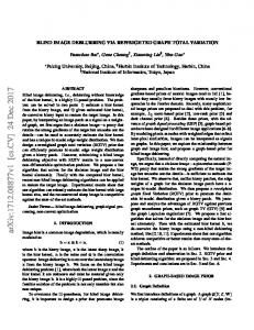
In all the experiments, we use q = 1/2, λ0 = 0.5, α = 1/2, and the following setting for the two ADMM algorithms: (a) the image estimate (line 3 of Algorithm 1) is computed with 20 iterations of (j) the algorithm explained in Subsection 3.1, initialized with d0 = 0, (j)  (where x  is the estimate from the previous outer itu0 = G(j) x eration of Algorithm 1), μ = 0.5, and ρ = 2λ; (b) the filter estimate (line 4 of Algorithm 1) is computed with 15 iterations of the (j) algorithm explained in Subsection 3.2, initialized with d0 = 0, (j) (j)   u0 = G h (where h is the filter estimate from the previous outer iteration), μ(1) = 0.01, and μ(2) = 0.1; (c) all the ADMM penalty parameters (μ(j) ) are updated using the empirical rule described in [10]. Both the proposed method and the method of [4] (implemented in MATLAB and run on an Intel Core i3 CPU) were stopped at the best ISNR (improvement in signal to noise ratio1 ), in the synthetic experiments, or at the best visual result, for the real images. The proposed approach was compared against its ancestor [4], in a set of 30 synthetic experiments with two benchmark images (Lena and Cameraman), five 9 × 9 blur kernels (see Fig. 1), at three noise levels (BSNR ∈ {∞, 40, 30}dB). Instead of periodic boundary conditions, we extended the images with values equal to the nearest boundary and both methods were run assuming unknown boundaries (see Subsection 2.1). For most experiments, the proposed method led to considerably higher ISNR, while being more than three times faster; even higher speed-ups are expected if the fixed number of iterations is replaced by adequate stopping criteria. The average ISNR and processing times in Table 1 show that the proposed method clearly outperforms the baseline from [4].

j=1

if the convolutions with the edge filters represented by the matrices Fi are performed with periodic boundary conditions, K can be efficiently computed in the DFT domain (using the FFT), since both H and F are block-circulant matrices (see [1, 2], for details). To implement line 6 of Algorithm 2, we need the two PO: λ 1 xq2 + v − x22 μ 2

 = v-shrink v, λ/μ, q ,

proxg(j) /μ (v) = arg min x

(10)

for j = 1, ..., m, and (with I denoting an identity matrix) 2 1 2 1 proxg(m+1) /ρ (v) = arg min y − Mx 2 + v − x 2 x ρ 2

−1 T  M y + ρv . = ρ I + MT M (11) The proximity operator in (11) can be easily computed: MT M is a binary diagonal matrix, with zeros corresponding to the unobserved boundary pixels, and MT y is the extension of y ∈ Rn to Rm by zero-padding. Finally, “v-shrink” in (10) is a vectorial shrinkage function, which can be shown (details are omitted) to be given by 

 y shrink 1, τ yq−2 2 , q if y2 = 0 v-shrink(y, τ, q) = (12) 0 if y2 = 0 where shrink(z, τ, q) = arg minx 12 z − x22 + τ |x|q has closed form solutions for q ∈ {0, 1/2, 2/3, 1, 4/3, 3/2, 2} (in some cases as functions of the roots of cubic and quartic equations [12]).

3.2. Updating the Blur Estimate

Fig. 1. Blurring filters used in the synthetic experiments: out-offocus, linear motion, square, nonlinear motion, and Gaussian.

The blur estimate update problem of Algorithm 1 (line 4) can be written in unconstrained formulation as 1 min y − MXh22 + ιS + (h), h 2

Table 1. Comparison between the baseline method [4] and our ADMM approach. The results for each BSNR value are averages over the five blurring filters and two images (Lena and Cameraman). ISNR (dB) time (s) BSNR (dB) [4] Proposed [4] Proposed

and in constrained form (3), with J = 2, G(1) = X, G(2) = I, and g (1) (u(1) ) =

1 y − Mu(1) 22 , 2

 g (2) u(2) = ιS + (u(2) ), (13)

∞ 40dB 30dB

where h ∈ Rm is the vector containing the blurring filter elements (lexicographically ordered) and X ∈ Rm×m is the square matrix representing the convolution of image x with the filter in h. The resulting instance of Algorithm 2 involves (in line 4) the inversion of the matrix μ(1) XT X + μ(2) I which can be efficiently computed in the DFT domain, using the FFT. Concerning the two (J = 2) proximity operators in line 6, we have that proxg(1) /μ(1) has exactly the same form as (11), with μ replacing ρ. Finally, since the proximity operator of the indicator of a convex set is simply the

5.83 4.95 3.83

8.87 6.65 5.01

249 131 110

69 55 46

Fig. 2 shows results obtained with a real motion blurred photo, using several BID methods: the proposed approach, that of [4], and two recent state-of-the-art methods proposed in [15, 17] (available at 1 ISNR is computed as in [4], after compensating for possible shifts and affine transformations of the intensity values.

588

Blurred photo.

[4], 138 seconds.

[15], 285 seconds.

[17], 177 seconds.

Our method, 62 seconds.

Fig. 2. Real blurred image and deblurred images (estimated blurs are shown in inset at the bottom right corner of each image), obtained by several methods (image size: 256 × 200; blur support: 23 × 23). forms several state-of-the-art methods, both in terms of speed and restoration quality. Ongoing research aims at developing adequate stopping criteria for the inner ADMM algorithms, as well as for the outer iterations, namely following our recent work in [6]. 6. REFERENCES [1] M. Afonso, J. Bioucas-Dias, M. Figueiredo, “Fast image recovery using variable splitting and constrained optimization,” IEEE Trans. Image Proc., vol. 19, pp. 2345–2356, 2010. a) Observed photo.

[2] ——, “An augmented Lagrangian approach to the constrained optimization formulation of imaging inverse problems,” IEEE Trans. Image Proc., vol. 20, pp. 681–695, 2011. [3] M. Almeida, A. Abelha, L. Almeida, “Multi-resolution approach for blind deblurring of natural images,” in IEEE ICIP, 2012. [4] M. Almeida, L. Almeida, “Blind and semi-blind deblurring of natural images,” IEEE Trans. Image Proc., vol. 19, pp. 36–52, 2010.

c) [4], 210 seconds.

[5] M. Almeida, M. Figueiredo, “Deconvolving images with unknown boundaries using the alternating direction method of multipliers,” IEEE Trans. Image Proc., vol. 22, 2013.

d) Our method, 75 seconds.

[6] M. Almeida, M. Figueiredo, “New stopping criteria for iterative blind image deblurring based on residual whiteness measures,” in IEEE Statist. Sig. Proc. Worksh., 2011, pp. 337–340.

Fig. 3. Actual photo with out-of-focus blur. Results obtained, with several BID methods. Image size: 256 × 256. Filter size: 13 × 13.

[7] B. Amizic, S. Babacan, R. Molina, A. Katsaggelos, “Sparse Bayesian blind image deconvolution with parameter estimation,” in European Signal Processing Conference, 2010.

tinyurl.com/a2ltbu4 and tinyurl.com/avuw5bk), with their parameters manually adjusted for the visually best result. Besides being considerably faster, our method attained the best restoration, yielding an image with sharp edges and no significant artifacts. Fig. 3 shows results obtained with an actual photo out-of-focus using the proposed approach and its ancestor method [4]. Our method attained a sharper image within one third of the processing time.

[8] S. Babacan, R. Molina, A. Katsaggelos, “Variational Bayesian blind deconvolution using a total variation prior,” IEEE Trans. Image Proc., vol. 18, pp. 12–26, 2009. [9] S. Cho, S. Lee, “Fast Motion Deblurring,” ACM Transactions on Graphics (SIGGRAPH ASIA 2009), vol. 28, 2009. [10] S. Boyd, N. Parikh, E. Chu, B. Peleato, d J. Eckstein, “Distributed optimization and statistical learning via the alternating direction method of multipliers,” Foundations and Trends in Machine Learning, vol. 3, pp. 1–122, 2011.

5. CONCLUSIONS AND ONGOING WORK We have proposed a new algorithm for blind deconvolution, improving over the recent method of [4] in two ways: a significant speedup (by using the ADMM) and the ability to handle unknown boundary conditions (more realistic than the usual periodic ones). Experiments with synthetic and real blurred images show that our method outper-

[11] J.-F. Cai, H. Ji, C. Liu, Z. Shen, “Framelet-based blind motion deblurring from a single image,” IEEE Trans. Image Proc., vol. 21, pp. 562 – 572, 2012.

589

[12] P. Combettes, J.-C. Pesquet, “Proximal splitting methods in signal processing,” in Fixed-Point Algorithms for Inverse Problems in Science and Engineering, H. Bauschke et al, Editors, Springer, 2011, pp. 185–212. [13] R. Fergus, B. Singh, A. Hertzmann, S. Roweis, W. Freeman, “Removing camera shake from a single photograph,” ACM Trans. Graph., vol. 25, pp. 787–794, 2006. [14] D. Gabay, B. Mercier, “A dual algorithm for the solution of nonlinear variational problems via infinite element approximations,” Comp. and Math. with Appl., vol. 2, pp. 17–40, 1976. [15] D. Krishnan, T. Tay, R. Fergus, “Blind deconvolution using a normalized sparsity measure,” in IEEE CVPR, 2011. [16] A. Levin, Y. Weiss, F. Durand, W. Freeman, “Understanding and evaluating blind deconvolution algorithms,” in IEEE CVPR, 2009. [17] ——, “Efficient marginal likelihood optimization in blind deconvolution,” in IEEE CVPR, 2011. [18] W. Li, Q. Li, W. Gong, S. Tang, “Total variation blind deconvolution employing split Bregman iteration,” J. Vis. Comun. Image Represent., vol. 23, pp. 409–417, 2012. [19] R. Liu, J. Jia, “Reducing boundary artifacts in image deconvolution,” in IEEE ICIP, 2008. [20] J. Miskin, D. MacKay, “Ensemble learning for blind image separation and deconvolution,” in Proc. Int. Worksh. Independ. Comp. Analysis and Blind Source Separation – ICA, 2000. [21] Q. Shan, J. Jia, A. Agarwala, “High-quality motion deblurring from a single image,” ACM Trans. Graph., vol. 27, 2008. [22] C. Wang, L. Sun, Z. Chen, J. Zhang, S. Yang, “Multi-scale blind motion deblurring using local minimum,” Inverse Problems, vol. 26, 2010. [23] L. Xu, J. Jia, “Two-phase kernel estimation for robust motion deblurring,” in ECCV, 2010.

590