Blind Inversion in Nonlinear Space-Variant Imaging by Using Cauchy Machine Ivica Kopriva and Harold Szu Digital Media RF Laboratory Department of Electrical and Computer Engineering-Room 308 George Washington University 725 23rd Street NW, Washington DC 20052, USA e-mail:
[email protected] ABSTRACT A Cauchy Machine has been applied to solve nonlinear space-variant blind imaging problem with positivity constraints on the pixel-by-pixel basis. Nonlinearity parameters, de-mixing matrix and source vector are found at the minimum of the thermodynamics free energy H=U-T0S, where U is estimation error energy, T0 is temperature and S is the entropy. Free energy represents dynamic balance of an open information system with constraints defined by data vector. Solution was found through Lagrange Constraint Neural Network algorithm for computing the unknown source vector, exhaustive search to find unknown nonlinearity parameters and Cauchy Machine for seeking demixing matrix at the global minimum of H for each pixel. We demonstrate the algorithm capability to recover images from the synthetic noise free nonlinear mixture of two images. Capability of the Cauchy Machine to find the global minimum of the ‘golf hole’ type of landscape has hitherto never been demonstrated in higher dimensions with a much less computation complexity than an exhaustive search algorithm.
Index terms – Cauchy machine, Helmholtz free energy, space-variant imaging, blind inversion, sensor nonlinearities. 1.0 INTRODUCTION 3,4,5,6
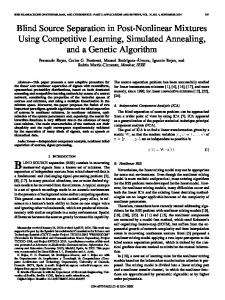
Cauchy Machine developed by Szu could be viewed as a fast version of the simulated annealing algorithms. Indeed, Geman & Geman2 had proved that simulated annealing algorithm based on Boltzmann thermal noise, i.e. Boltzmann Machine1 would require a slow cooling schedule at the inversely logarithmic in time steps. Szu et al. in Ref. 3-6 had proved that Cauchy color noise, rather than Boltzmann thermal noise, could achieve the global optimization in a much faster cooling schedule that is inversely linear in time steps. This Fast Simulated Annealing (FSA) theory helped build optical Cauchy Machine (CM) for NASA spectral search with Scheff and Landa7, and solve the necessary and sufficient constraints of Traveling Salesman Problems (TSP) by Szu6. Important novelty of this paper is application of the CM to unsupervised classification and implementation of the 2D Cauchy machine to find the global minimum of the ‘golf hole’ type of landscape that arises in blind inversion of the single pixel space-variant imaging problems, Szu and Kopriva8-11, right side on Figure 1. In the ‘ocean’ type landscape, left side on Figure 1, the single minimum can be found by ordinary deterministic gradient descent algorithm. However, constrained optimization problems very often result in multiple minimums with the ‘lake’ type of landscape, middle of the Figure1, or ‘golf hole’ type of landscape, right side of the Figure 1. For such cases the gradient descent algorithm will be trapped in some of the local minimums. Stochastic search based on simulated annealing theory1-4 enables non-convex optimization algorithm to escape from the local minima. It has been proven that convergence of the stochastic search based on the Cauchy distribution with unbounded variance (Cauchy Machine)3-4, is inversely proportional with time while convergence of the
1
stochastic search algorithms based on Gaussian distribution (Boltzmann Machine)1 is inversely proportional with the logarithmic function of time2. Convergence of the Cauchy Machine has been demonstrated in4 for a 1D double-well potential function the 2D equivalent of which is shown in the middle of the Figure 1 (the ‘lake’ type of landscape). However, the Helmholtz free energy based objective function used in blind spacevariant imaging problems8 has from the global optimization point of view a very difficult ‘golf hole’ type of landscape, right side on Figure 1.
Figure 1. From left to right are 2D objective functions with ocean like landscape; multiple lakes like landscape; golf hole like landscape. The last one arises in blind inversion of the space-variant imaging problem minimising thermodynamic free energy with physics constraints defined by data vector.
We demonstrate in this paper, according to our knowledge for the first time, application of the 2D Cauchy Machine on the global minimization of the ‘golf hole’ type of landscape which comes from the real world constrained optimization problem such as blind de-mixing of the nonlinear space-variant mixture of images8-12. New solution for deterministic blind space-variant imaging problem is proposed as a marriage of the unsupervised feed-forward type of the Lagrange Constraint Neural Network (LCNN)8,10-12 to find unknown source vector, Figure 2, exhaustive search to find nonlinearity parameters and 2D Cauchy Machine8 to find de-mixing matrix. Unlike statistical independent component analysis (ICA) algorithms14-18 solution is deterministic and solves the problem on the pixel by pixel basis. Hence, we may assume blind inversion nonlinear imaging problem to be space-variant.
Figure 2. A Feed-forward Lagrange Constraint Neural Network8,9,10. Brief description of the blind nonlinear space-variant imaging problem is given in Section 2. Provided that nonlinearity is a monotonic function with unique inverse this allows extension of the application of essentially the same contrast function from linear case8 to nonlinear one which is reported here. Here we propose solution that is deterministic and solves the nonlinear problem on the pixel by pixel basis. Hence, we may assume unknown mixing matrix to be space-variant which is important property for detection of small objects on the sub-pixel level that happens both in remote sensing11,21,26 and thermography based
2
early cancer detection27. Section 3 briefly describes application of the 2D version of the FSA algorithm based on the Cauchy Machine theory3,4 on the blind space-variant imaging problem while more details can be found in Ref. 8. In Section 4 we demonstrate capability of the 2D Cauchy Machine to find the global minimum of the very difficult ‘golf hole’ type of landscape as well as demonstrate the algorithm capability to recover images from the synthetic noise free nonlinear mixture of two images. Conclusion is given in Section 4. 2.0 BLIND NONLINEAR SPACE-VARIANT IMAGING PROBLEM The noise free blind nonlinear space-variant imaging problem is defined as:
r r X ( p ,q ) = g [ A]( p ,q ) S ( p ,q )
(
)
(1) r r where g(o) is nonlinear function that models sensor nonlinearity and X and S are n and m dimensional column vectors representing measured data and unknown sources respectively with m ≤ n and [A] being nxm unknown mixing matrix. The subscript (p,q) denotes spatial coordinates i.e. the blind space-variant imaging problem is formulated on the pixel by pixel basis. Note that such formulation allows the mixing matrix [A](p,q) to be spatially variant. We shall drop (p,q) subscript in the subsequent derivations in order to simplify notation. The solution of the nonlinear blind imaging problem is to find both the unknown mixing r r matrix [A] and unknown source vector S based on the given data vector X only. The linearized version of the nonlinear mixture (1) is obtained as: r r r r ~ (2) X = g −1 X = g −1 g [ A]S ≅ [ A]S In reality the nonlinearity parameters are unknown and have to be estimated through some optimization r r ~ process. Because both X and S have the physical interpretation of intensity the positivity constraint is imposed on them: ~ xi ≥ 0 i = 1,..., n (3) si ≥ 0 i = 1,..., m If the unknown mixing matrix has physical interpretation of the spectral reflectance matrix as in remote sensing21,27 or point spread function of the optical or non-optical imaging system25 than positivity constraints must be imposed on [A] too: aij ≥ 0 i = 1,.., n; j = 1,.., m (4)
( )
((
))
We shall rewrite (2) in a slightly different form: r r ~ X = [ A]NS , where:
(5)
N = ∑ im=1 si
(6)
s (7) si, = i N With (6) we have introduced unknown scaling factor N that helped us to assign to the components of the r scaled source vector S , the meaning of probability because due to (6)-(7) they satisfy the constraint: m ∑i =1 s i, = 1
(8)
We now formulate the Helmholtz free energy as contrast function with probability constraint (8) taken into account explicitly as: r r r r r H (α , [W ], S ) = U − T0 S = µ T [W ]g −1 X − NS , + K B T0 N ∑im=1 s i, ln si, + N ( µ 0 − K B T0 ) ∑im=1 si, − 1 (9)
[
( )
]
(
)
where Shannon entropy was approximated by:
S = − K BT0 ∑ im=1 si, ln si,
(10)
3
where KB represents Boltzmann’s constant and T0 represents temperature. They are introduced in (9) due to r dimensionality reasons. µ in (9) is a vector of Lagrange multipliers that in our formalism has interpretation of the virtual forces. We remark here that our contrast function (9) is equivalent to the formulation of the solution of problem (5) using the principle of maximum entropy23,24, which gives as a solution distribution r r r p (S ) with the maximal entropy under given macroscopic constraints U = [W ] g −1 X − NS , defined by r measured data X :
(
)
( )
∑i =1 w ji g i−1 ( xi ) = Ns ,j n
(11)
where [W] is an mxn unmixing matrix and for the case m=n [W ] = [ A]−1 . We remark here that in relation to the linear deterministic BSS algorithm described in Ref. 8 the contrast function (9) includes also vector of r the unknown nonlinearity parameters α . Essential difference between our algorithm and classical maximum 23,24 is that problem (1) is nonlinear with unknown mixing matrix [A] or the unmixing entropy solution r matrix [W] and unknown nonlinearity parameters α . To solve the nonlinear BSS imaging problem with the positivity constraints we formulate an algorithm as a combination of the global optimization algorithm that looks for the global minimum of the error energy function: r T r r r r α * , [W * ], N * = arg min [W ] g −1 ( X ) − NS , [W ]g −1 ( X ) − NS , (12) r r, 8 and MaxEnt like algorithm for finding the most probable distribution p ( S ) = S for a given r triplet α (l ) , [W (l) ], N (l) where l denotes iteration index in a solution of problem (12). Here the vector of r nonlinearity parameters α is found by using exhaustive search algorithm and unkown de-mixing matrix is found by using fast simulated annealing algorithm based on the 2D Cauchy Machine8. Figure 3 gives an illustration how nonlinear deterministic blind inversion algorithm works. At some iteration l triplet r α (l ) , [W ](l ) , N (l ) is generated as an output of the optimization algorithm in an attempt to reach possibly r global minimum of the estimation error energy (12). For a given triplet α (l ) , [W ](l ) , N (l ) the MaxEnt r r algorithm described in Ref. 8 computes the most probable solution for the source vector S (l ) = N (l ) S ,(l ) . This represents feedback for the optimization algorithm that computes a new value of the estimation error r energy and generates a new triplet α (l +1) , [W ](l +1) , N (l +1) . After each iteration l is completed we get a r r quadruple α (l ) , [W ](l ) , N (l ) , S ,(l ) . Algorithm accepts as a final solution the quadruple r r α * , [W ]* , N * , S ,* for which the estimation error energy (12) reaches a possibly global minimum. r r Provided that nonlinear function g() has unique inverse the quadruple α * , [W ]* , N * , S ,* , corresponding with given data model (1), will give a global minimum of the error energy function.
(
)
(
)(
)
)
(
(
(
)
(
(
)
)
(
)
)
(
)
Figure 3. Illustration of the blind inversion of nonlinear space-variant imaging problem.
4
3. 2D CAUCHY MACHINE SIMULATED ANNEALING ALGORITHM The full description of the application of the 2D Cauchy Machine on the space-variant imaging problem can be found in Ref. 9 while summarized version will be presented here. As in Ref. 8 we model 2D spacevariant imaging problem by using two mixing angles θ and ϕ :
x x cos θ cos ϕ s ,x (13) = N , sin θ sin ϕ s y x y Based on (13) the unknown de-mixing matrix [W] is described by two ‘killing’ angles ξ and ζ as8: r cos ξ sin ξ w1 1 (14) [W ] = = r sin(ζ − ξ ) cos ζ sin ζ w 2 Vector diagram representation of the mixing model (3)/(13)/(14) is shown on Figure 4. The unknown demixing matrix [W] is found at a global minimum of the Helmholtz free energy objective function (9)/(12) using FSA based on 2D Cauchy Machine. Therefore a 2D Cauchy probability density function (pdf) in the killing angles domain is defined3,4: K c (15) p (ς ,ξ ) = 1 K 2 ς 2 +ξ 2 + c 2 3/ 2
where K1 and K2 are normalization constants to be determined. Due to the positivity constraints (3) the killing angles lie in the domain: π π ς ∈ , π ξ ∈ − , 0 (16) 2 2 If, based on Figure 4, we adopt the convention that for original mixing angles θ and ϕ it applies the following: ϕ ≤ χ ≤θ (17) r where χ is angle defined by data vector X as: x χ = tan −1 x (18) xy than domain of support for killing angles is narrowed according to: π π π (19) ς ∈ + χ , π ξ ∈ − ,− + χ 2 2 2 which reduces the size of the search space. The 2D pdf (15) can be transformed from the Cartesian p (ζ ,ξ ) to polar p (r , ω ) coordinates using standard transformation from Cartesian to polar coordinate system. Geometry relations between Cartesian (ξ , ζ ) and polar (r ,θ ) coordinate systems are illustrated on Figure 5. Due to (19) the angle polar coordinate ω lies in: ω min ≤ ω ≤ ω max (20) where ωmin and ωmax are defined with: π χ +π 2 ω max = tan −1 ω min = tan −1 (21) χ −π 2 −π 2 The radial coordinate r lies in: r ∈[rmin , rmax ] (22) where rmin and rmax are given for a particular value of ω with: χ +π 2 rmin = sin ω
5
rmax
π ω ∈ [ω min , π + tan −1 (−2)] sin ω = − π ω ∈[π + tan −1 (−2), ω max ] 2 cos ω
Figure 4. Vector diagram representation of the mixing model (3)/(13)/(14).
Figure 5. Geometry relations between Cartesian (ξ , ζ ) and polar (r , ω ) coordinates
Cartesian pdf p(ζ , ξ ) (15) can be written in polar coordinates p (r , ω ) as: cr p (r , ω ) = p (ω ) p (r ) = K1 K 2 3/ 2 2 r + c2 It has been derived in Ref. 8 that p (ω ) takes the form: 1 p (ω ) = K 1 = ω max − ω min and: ω = (ω max − ω min )x + ω min
(
(23)
)
(24)
(25)
(26)
where integration constant x is random variable uniformly distributed on the interval [0,1]. Also from Ref. 8 p(r) takes the form: c r p (r ) = (27) K 2 r 2 + c 2 3/ 2
(
)
where normalization constant K2 is given with: 1 1 − K 2 = c 2 r 2 + c2 rmax + c 2 min
(28) Random variable r is generated based on the uniformly distributed random variable x on some interval [xmin,xmax] and through relation:
6
r=
c 1 − K 22 x 2 K2x
(29)
where: 1
xmin = K2
2 1 + rmin
xmax =
1 2 K 2 1 + rmax
(30)
Relation between random variable x uniformly distributed on the interval [xmin, xmax] and random variable ~ x uniformly distributed on the interval [0, 1] is given through: (31) x = (xmax − xmin )~ x + xmin Like in Boltzmann Machine based simulated annealing algorithm1 the new solution in terms of killing angles (ξ , ζ ) at some iteration k is accepted if either: H (k ) < H (k − 1)
(32)
or if Metropolis criteria1 is satisfied: 1 pk ≤ − ∆Ek / T (1 + e )
(33)
where pk is uniformly generated probability and ∆E k = H (k ) − H ( k − 1) is positive error energy at iteration k. Metropolis criteria (33) avoids algorithm to escape from local minima even if value of the Helmholtz free energy at iteration k is greater than value at the previous iteration. 4.0 SIMULATION RESULTS We demonstrate performance of the nonlinear blind inversion algorithm modeling sensor nonlinearity using following function:
(
)
xin = g ( xi ) = 2 B 1 − e −α i xi (34) where B in Eq.(34) represents number of bits and αi is an unknown slope. For our simulation demo we have assumed B=8 and α i = 0.01 to be nominal value of the nonlinearity slope but we allowed drift from the nominal value in some ±10% interval around nominal value. The inverse of the nonlinear function (34) is given by: 1 1 ln (35) g −1 ( xin ) = αi xn 1 − iB 2 Two 72x88 images were mixed by a mixing matrix that has been changed from pixel to pixel in order to simulate the space-variant imaging problem. Angles θ and ϕ are changed column wise according to Figure 6 i.e. for every column index angles were changed for 10 and mutual distance between them was 40. Figure 7 shows number of iteration necessary for 2D Cauchy Machine algorithm (15)-(33) to find global minimum of the ‘golf hole’ type of error energy function (12) for 100 runs. Solid line on Figure 7 represents fixed number of iteration required by exhaustive search algorithm that in this example is 1972. The average number of iteration per run using 2D Cauchy simulated annealing algorithm was 1684 while exhaustive search required 1972 iterations to find solution. This gives an estimate of the speed-up factor as 1972/1684≈1.171 or 17%. Results presented on Figure 8 show from left to right two source images, two linearly mixed images, two images after linear mixture has been passed through nonlinearity (34) and two separated images using blind inversion algorithm (9)-(12)-(33). Thanks to the fact that blind inversion algorithm solves the problem on the pixel-by-pixel basis the recovery was almost perfect although mixing matrix was space-variant. We have compared our result with the two representative stochastic ICA methods that were applied on the same mixture shown on Figure 6 as well as linear version of the deterministic blind inversion algorthm8. Separation results of the Bell-Sejnowski Infomax algorithm15, Cardoso’s JADE algorithm17 and linear deterministic BSS algorithm8 are shown on Figure 9. Due to the space-variant and nonlinear nature of the mixing matrix ICA algorithms15,17 fail to recover the original images. The same is
7
true for linear deterministic blind inversion algorithm8 due the nonlinear nature of the mixture. Figure 10 shows difference images obtained after recovered images were subtracted from the original source images. From left to right are difference images obtained by nonlinear blind inversion algorithm (9)-(12)-(33), linear deterministic blind inversion algorithm8, Infomax algorithm15 and JADE algorithm17. As could be seen from Figure 10 in a case of last three algorithms a lot of information is contained in difference images suggesting that reconstructed images shown on Figure 9 are of the poor quality. Results are summarized on Figure 11 that shows logarithm of the Mean Square Error (MSE) defined by:
∑i =1 ∑ x =1 ∑ y =1 (sˆ ix, y − s xi , y ) 2
MSE =
p
q
2 pq
2
(36)
Before computing MSE (36) effects of the scaling and permutation indeterminacies characteristic for ICA algorithms has been taken into account and corrected.
Figure 6. Change of the angles vs. column index. Solid line - ϕ angle; dashed line - θ angle.
Figure 7. Number of iterations per run for overall 100 runs necessary to find global minimum of the error energy function (12) by using 2D Cauchy Machine FSA algorithm (15)-(33) (dashed line)
Figure 8. From left to right: source images; space-variant noise free linear mixture; space-variant noise free nonlinear mixture; recovery of the source images using nonlinear blind inversion algorithm (9)-(12)-(33).
8
Figure 9. Recovered images from the space-variant nonlinear mixture shown on Figure 6. From left to right: linear deterministic blind inversion algorithm8; Infomax ICA algorithm15; JADE ICA algorithm17.
Figure 10. Difference images for image recovery from the space-variant nonlinear mixture shown on Figure 6. From left to right: nonlinear blind inversion algorithm (9)-(12)-(33), linear deterministic blind inversion8; Infomax ICA algorithm15; JADE ICA algorithm17.
9
Figure11. MSE (36) for: 1- nonlinear blind inversion algorithm (9)-(33); 2-linear deterministic blind inversion algorithm8; 3Infomax ICA algorithm15 and 4 - JADE ICA algorithm17.
Method
MSE
Nolinear deterministic BSS
0.1321
Linear deterministic BSS Infomax JADE
118.7438 58.7842 118.5232
Table 1. MSE for different blind inversion methods.
5.0 CONCLUSION AND FUTURE WORK A 2D Cauchy Machine based algorithm capable of solving noise free space-variant imaging problem with sensor nonlinearities on the pixel-by-pixel basis has been presented. This is accomplished by the two stage algorithm that combines minimization of the thermodynamics Helmholtz free energy with the maximum entropy based algorithm that for each pixel computes the most probable value of the source vector under given macroscopic constraints defined by data vector. Because of the ‘golf hole’ type of landscape of this objective function it is almost impossible to reach it by means of the gradient descent algorithms. It has been demonstrated that 2D Cauchy Machine is capable to find a global minimum in such a perfect recovery of images from the synthetic noise free space-variant nonliner mixture of two images. Due to difficult landscape under significantly less computational time than exhaustive search technique. Performance of blind inversion nonlinear algorithm has been demonstrated on the recovery of images from the synthetic noise free space-variant nonlinear mixture of two images. Due to the both nonlinear and space variant nature of the mixture linear deterministic blind inversion algorithm as well as stochastic ICA algorithms fail to recover unknown source images. The algorithm capability to recover source signals on the pixel-by-pixel basis is important for detection of small objects on the sub-pixel level which is a case in both remote sensing and thermography based early cancer detection. Future work will be directed toward fast simulated annealing methods necessary to solve higher dimensional (more than 2D) problems; noisy linear and nonlinear space-variant mixtures; testing of some other types of nonlinearity as well as testing of linear and nonlinear blind inversion algorithms on various types of applications.
ACKNOWLEDGMENT We acknowledge the financial support from the Office of Naval Research, Mr. James Buss, for the Grant BAA 02-001.
10
6.0 REFERENCES 1. Ackley, D.H., Hinton, G.E. and Sejnowski, T.J, “A learning algorithm for Boltzman Machines”, Cognitive Science 9, 147-169, 1985. 2. S. Geman and D. Geman, "Stochastic relaxation, Gibbs distribution and the Bayesian restoration of images," IEEE Transactions on Pattern Analysis and Machine Intelligence, vol. PAMI-6, no. 6, pp. 721741, November 1984. 3. H. Szu and R. Hartley, “Nonconvex Optimization by Simulated Annealing,” Proc. IEEE, 75, No. 11, 1987, 1538-1540. 4. H. Szu and R. Hartley, “Fast Simulated Annealing,” Physics Letters A, 122, No. 3, 1987, 157-162. 5. Y. Takefuji and H. Szu, “Design of Parallel Distributed Cauchy Machines,” International Joint Conf. Neural Networks, Washington, DC, 1989, pp. I-529-I-532. 6. H. Szu, “Colored Noise Annealing Benchmark by Exhaustive Solutions of TSP,” International Joint Conf. Neural Networks, Washington, DC, 1990, pp. I-317-I-320. 7. J. Landa, K. Scheff and H. Szu, “Binocular Fusion Using Simulated Annealing,” IEEE First Annual Conf. on Neural Networks, San Diego, 1987 .
8. H. Szu and I. Kopriva, “Deterministic Blind Source Separation for Space Variant Imaging,” accepted for the Fourth International Symposium on Independent Component Analysis and Blind Signal Separation, Nara, Japan, April 1-4, 2003. 9. H. Szu and I. Kopriva, “Cauchy Machine for Blind Inversion in Linear Space-Variant Imaging,” submitted for the 2003 International Joint Conference on Neural Networks, July 20-24, Portland, Oregon, USA, July 20-24, 2003. 10. H.H.Szu and I.Kopriva, “Comparison of the Lagrange Constrained Neural Network with Traditional ICA Methods,” Proc. of the 2002 World Congress on Computational Intelligence-International Joint Conference on Neural Networks, pp. 466-471, Hawaii, USA, May 17-22, 2002. 11. H. H. Szu and C. Hsu, “Landsat spectral Unmixing à la superresolution of blind matrix inversion by constraint MaxEnt neural nets,” Proc. SPIE 3078, pp.147-160, 1997. 12. H. Szu, “A Priori Maxent H(S) Independent Class Analysis (Ica) Vs. A Posteriori Maxent H(V) Ica,” Proc. of the 3rd International Workshop on BSS and ICA, San Diego, USA, December 9-13, 2001, ed. Lee, Jung, Makeig, Sejnowski, pp. 80-89. 13. Szu, H. Thermodynamics energy for both supervised and unsupervised learning neural nets at a constant temperature. Int’l J. Neural Sys. 9, 175-186 (1999). 14. S. Amari, A. Cihocki, H. H. Yang, “A new learning algorithm for blind signal separation,” Advances in Neural Information Processing Systems, 8, MIT Press, 757-763, 1996. 15. A. J. Bell and T. J. Sejnowski, “An information-maximization approach to blind separation and blind deconvolution,” Neural Comp. 7, 1129-1159 , 1995. 16. A. Hyvärinen and E. Oja, “A fast fixed-point algorithm for independent component analysis,” Neural Computation, vol. 9, pp. 1483-1492, 1997. 17. J. F. Cardoso, A. Soulomniac, “Blind beamforming for non-Gaussian signals,” Proc. IEE F, vol. 140, pp. 362-370, 1993. 18. M. Plubmley, “Conditions for Nonnegative Independent Component Analysis,” IEEE Sig. Proc. Let., vol. 9, No. 6, June, 2002, pp.177-180. 19. J. W. Miskin, D. J. MacKay, “Application of Ensemble Learning ICA to Infra-Red Imaging,” Proc. of the 2nd International Workshop on ICA and BSS, Helsinki, Finland, June, 2001, ed. P. Pajunen and J. Karhunen, pp. 399-404. 20. D. D. Lee and H. S. Seung, “Learning the parts of objects by non-negative matrix factorization,” Nature, vol. 401, No. 21, pp.788-791, 1999. 21. L. Parra, C. Spence, P. Sajda, A. Ziehe, K-R. Müller, “Unmixing Hyperspectral Data,” in Advances in Neural Information Processing Systems (NIPS12), S. A. Jolla, T. K. Leen and K-R. Müller (eds), MIT Press, 2000. 22. K. Huang, “Statistical Mechanics,” J. Wiley, 1963. 23. E.T. Jaynes, “Information Theory and Statistical Mechanics,” Phys. Rev., 106, 620-630, 1957.
11
24. G. Deco and D. Obradovic, “Statistical Physics Theory of Supervised Learning and Generalization”, Chapter 8 in “An Information-Theoretic Approach to Neural Computing”, Springer, 1995, pp. 187-213. 25. H. H. Szu, I. Kopriva, “Artificial Neural Networks for Noisy Image Super-resolution,” Optics Communications, Vol. 198 (1-3) pp. 71-81, 2001. 26. B. F. Jones, “A Reappraisal of the Use of Infrared Thermal Image Analysis in Medicine,” IEEE Trans. On Medical Imaging, vol. 17, No. 6, pp. 1019-1027, 1998. 27. C. I. Chang and D. C. Heinz, “Constrained Subpixel Target Detection for Remotely Sensed Imagery,” IEEE Trans. Geosci. Remote Sensing, vol. 38, no. 3, pp. 1144-1158, May 2000. 28. H. Yang, S. Amari, and A. Cihocki, “Information-theoretic approach to blind separation of sources in non-linear mixture,” Signal Process. 64, 291-300, 1998.
12