Nonlinear Blind Source Separation Using Hybrid Neural Networks* Chun-Hou Zheng1,2, Zhi-Kai Huang1,2, Michael R. Lyu3, and Tat-Ming Lok4 1
Intelligent Computing Lab, Institute of Intelligent Machines, Chinese Academy of Sciences, P.O.Box 1130, Hefei, Anhui , China 2 Department of Automation, University of Science and Technology of China 3 Computer Science & Engineering Dept., The Chinese University of Hong Kong, Hong Kong 4 Information Engineering Dept., The Chinese University of Hong Kong, Shatin, Hong Kong
[email protected]
Abstract. This paper proposes a novel algorithm based on minimizing mutual information for a special case of nonlinear blind source separation: postnonlinear blind source separation. A network composed of a set of radial basis function (RBF) networks, a set of multilayer perceptron and a linear network is used as a demixing system to separate sources in post-nonlinear mixtures. The experimental results show that our proposed method is effective, and they also show that the local character of the RBF network’s units allows a significant speedup in the training of the system.
1 Introduction Blind source separation (BSS) in instantaneous and convolute linear mixture has been intensively studied over the last decade. Most of the blind separation algorithms are based on the theory of the independent component analysis (ICA) when the mixture model is linear [1,2]. However, in general real-world situation, nonlinear mixture of signals is generally more prevalent. For nonlinear demixing [6,7], many difficulties occur and the linear ICA is no longer applicable because of the complexity of nonlinear parameters. In this paper, we shall in-deep investigate a special but important instance of nonlinear mixtures, i.e., post-nonlinear (PNL) mixtures, and give out a novel algortithm.
2 Post-nonlinear Mixtures An important special case of the general nonlinear mixing model that consists of so called post-nonlinear mixtures introduced by Taleb and Jutten [5], can be seen as a hybrid of a linear stage followed by a nonlinear stage. *
This work was supported by the National Science Foundation of China (Nos.60472111, 30570368 and 60405002).
J. Wang et al. (Eds.): ISNN 2006, LNCS 3971, pp. 1165 – 1170, 2006. © Springer-Verlag Berlin Heidelberg 2006
1166
C.-H. Zheng et al.
s1 M sn
u1 A
un
x1
f1
M fn
Mixing system
g1
M
xn
gn
v1
y1 B
vn
M yn
Separating system
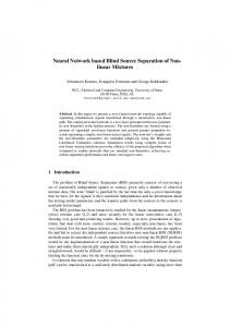
Fig. 1. The mixing –separating system for PNL
In the post-nonlinear mixtures model, the observations x = ( x1 , x2 ,L , xn )T have the following specific form (as shown in Fig. 1)
⎛ n ⎞ xi = f i ⎜ ∑ aij s j ⎟ , i = 1,L , n ⎝ j =1 ⎠
(1)
The corresponding vector-matrix form can be written as: x = f ( As )
(2)
Contrary to general nonlinear mixtures, the PNL mixtures have a favorable separability property. In fact, if the corresponding separating model for post-nonlinear mixtures, as shown in Figure 1, are written as: n
yi = ∑ bij g j ( x j )
(3)
j =1
Then it can be demonstrated that [5], under weak conditions on the mixing matrix A and on the source distribution, the output independence can be obtained if and only if ∀i = 1,L , n. , hi = gi o f i are linear. For more details, please refer to literatures [5].
3 Contrast Function In this paper, we use Shannon’s mutual information as the measure of mutual dependence. It can be defined as: I ( y ) = ∑ H ( yi ) − H ( y )
(4)
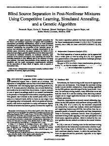
where H ( yi ) = − ∫ p( yi ) log p ( yi )dyi denotes Shannon’s differential entropy. According to the theory given above, the separating system of PNL we proposed in this paper is shown in Fig.2, where B and gi form the unmixing structure for PNL, yi are the extracted independent components, and ψ i some nonlinear mappings, which are used only for the optimization of the network.
Nonlinear Blind Source Separation Using Hybrid Neural Networks
1167
Assume that each function ψ i (φi , yi ) is the cumulative probability function (CPF) of the corresponding component yi , then zi are uniformly distributed in [0, 1], Consequently, H ( zi ) = 0 [7]. Moreover, because ψ i ( φ i , yi ) are all continuous and monotonic increasing transformations (thus also invertible), then it can be easily shown that I ( z) = I ( y ) [7]. Consequently, we can obtain
I ( y ) = I ( z ) = ∑ H ( zi ) − H ( z ) = − H ( z )
(5)
i
Therefore, maximizing H ( z ) is equivalent to minimizing I ( y ) .
x1
M ψ
x2
M
B
M
M ψ1
z1
y2
M ψ2
z2
M ψn
zn
g1
g2
M
M
xn
y1
yn gn
Fig. 2. The particular structure of the unmixing network
It has been proved in the literature [7] that, given the constraints placed on
ψ i (φi , yi ) , then zi is bounded to [0, 1], and given that ψ i ( φ i , yi ) is also constrained to be a continuous increasing function, then maximizing H ( z) will lead ψ i (φi , yi ) to become the estimates of the CPFs of yi . Consequently, yi should be the duplicate of si with just sign and scale ambiguity. Now, the fundamental problem that we should to solve is to optimize the networks (formed by the gi , B and ψ i blocks) by maximizing H ( z ) .
4 Unsupervised Learning of Separating System With respect to the separation structure of this paper, the joint probabilistic density function (PDF) of the output vector z can be calculated as: p( z) =
p(x ) n
n
i =1
i =1
det( B) ∏ g 'i (θi , xi ) ∏ ψ 'i (φi , yi )
(6)
which leads to the following expression of the joint entropy: n
n
i =1
i =1
H (z) = H (x) + log det(B) + ∑ E ( log g 'i (θi , xi ) ) + ∑ E ( log ψ 'i (φi , yi ) )
(7)
1168
C.-H. Zheng et al.
The minimization of I ( y ) , which is equal to maximize H ( z ) here, requires the computation of its gradient with respect to the separation structure parameters B , θ and φ . In this paper, we use RBF [3,4] network to model the nonlinear parametric functions g k (θ k , xk ) , and choose Gaussian kernel function as the activation function of the hidden neurons. In order to implement the constraints on the ψ function easy, we use multilayer perceptron to model the nonlinear parametric functions ψ k (φk , yk ) .
5 Experiment Results 5.1 Extracting Sources From Mixtures of Simulant Signals
In the first experiment, the source signals consist of a sinusoid signal and a funny curve signal [1], i.e. s(t ) = [(rem(t,27)-13)/9,((rem(t,23)-11)/9)0.5 ]T , which are shown in Fig.3 (a). The two source signals are first linearly mixed with the (randomly chosen) mixture matrix: ⎡-0.1389 0.3810 ⎤ A=⎢ ⎥ ⎣ 0.4164 -0.1221⎦
(8)
Then, the two nonlinear distortion functions
f1 (u ) = f 2 (u ) = tanh(u )
(9)
are applied to each mixture for producing a PNL mixture. Fig.3 (b) shows the separated signals. To compare the performance of our proposed method with other ones, we also use MISEP method [7] to conduct the related experiments based on the same data. The correlations between the two recovered signals separated by two methods and the two original sources are reported in Table.1. Clearly, the separated signals using the method proposed in this paper is more similar to the original signals than the other. 2
5
0
0
-2 0 5
0.2
0.4
0.6
0.8
1
0 -5 0
-5 0 5
0.2
0.4
0.2
0.4
0.6
0.8
1
0.6
0.8
1
0
0.2
0.4
0.6
(a)
0.8
1
-5 0
(b)
Fig. 3. The two set of signals shown. (a) Source signals. (b) Separated signals.
Nonlinear Blind Source Separation Using Hybrid Neural Networks
1169
Table 1. Correlations between two original sources and the two recovered signals
simulant signals
Experiment
MISEP Method in this paper
y2
y1
speech signals y1
y2
S1
0.9805 0.0275 0.9114 0.0280
S2
0.0130 0.9879 0.0829 0.9639
S1
0.9935 0.0184 0.9957 0.0713
S2
0.0083 0.9905 0.0712 0.9711
5.2 Extracting Sources from Mixtures of Speech Signals To test the validity of the algorithm proposed in this paper ulteriorly, we also have experimentalized using real-life speech signals. In this experiment two speech signals (with 3000 samples, sampling rate 8kHz, obtained from http://www.ece.mcmaster.ca /~reilly/ kamran /id18.htm) are post-nonlinearly mixed by: ⎡ -0.1412 0.4513 ⎤ A= ⎢ ⎥ ⎣ 0.5864 -0.2015⎦
f1 (u ) =
(10)
1 1 3 (u + u 3 ) , f 2 (u ) = u + tanh(u ) 2 6 5
(11)
The experimental results are shown in Fig.4 and Table.1, which conforms the conclusion drawn from the first experiment. 8
5
0
0 -5 0 5
0.2
0.4
0.6
0.8
1
0.2
0.4
0.6
0.8
1
0.2
0.4
0.6
0.8
1
0
0 -5 0
-8 0 9
0.2
0.4
0.6
(a)
0.8
1
-9 0
(b)
Fig. 4. The two set of speech signals shown. (a) Source signals. (b) Separated signals.
5.3 Training Speed
We also performed tests in which we compared, on the same post-nonlinear BSS problems, networks in which the g blocks had MLP structures. Table 2 shows the means and standard deviations of epochs required to reach the stop criterion, which was based on the value of the objective function H ( z ) , for MLP-based networks and RBF-based networks.
1170
C.-H. Zheng et al.
Table 2. Comparison of training speeds between MLP-based and RBF-based networks
Two superg supergaussions RBF MLP
Superg. and subg. RBF
MLP
Mean
315
508
369
618
St. dev
141
255
180
308
From the two tables we can see that the separating results of the two methods are very similar, but the RBF-based implementations trained faster and show a smaller oscillation of training times (One epoch took approximately the same time in both kinds of network). This mainly caused by the local character of RBF networks.
6 Conclusions We proposed in this paper a novel algorithm for post-nonlinear blind source separation. This new method works by optimizing a network with a specialized architecture, using the output entropy as the objective function, which is equivalent to the mutual information criterion but needs not to calculate the marginal entropy of the output. Finally, the experimental results showed that this method is competitive to other existing ones.
References 1. Hyvärinen, A., Karhunen, J., Oja, E.: Independent Component Analysis. J. Wiley, New York (2001) 2. Hyvärinen, A., Pajunen, P.: Nonlinear Independent Component Analysis: Existence and Uniqueness Results. Neural Networks, 12(3) (1999) 429–439 3. Huang, D.S.: Systematic Theory of Neural Networks for Pattern Recognition. Publishing House of Electronic Industry of China, Beijing (1996) 4. Huang, D.S.: The United Adaptive Learning Algorithm for the Link Weights and the Shape Parameters in RBFN for Pattern Recognition. International Journal of Pattern Recognition and Artificial Intelligence.11(6) (1997) 873-888 5. Taleb, A., Jutten, C.: Source Separation in Post- nonlinear Mixtures. IEEE Trans. Signal Processing, 47 (1999) 2807–2820 6. Martinez, Bray, D. A.: Nonlinear Blind Source Separation Using Kernels. IEEE Trans. Neural Networks, 14(1) (2003) 228–235 7. Almeuda, L. B.: MISEP – Linear and Nonlinear ICA Based on Mutual Information. Journal of Machine Learning Research.4(2) (2003) 1297-1318