Bloat and its control in Genetic Programming ... Dynamically computing parsimony penalty ... Large trees require memory
Bloat and its control in Genetic Programming Nic McPhee Division of Science and Mathematics University of Minnesota, Morris Morris, Minnesota, USA Currently on sabbatical working with Riccardo Poli, University of Essex, UK
13 June 2008 University of Granada
Nic McPhee (U of Minnesota, Morris)
Bloat control in GP
13 June 2008, U of Granada
1 / 21
Overview
The big picture
The big picture
Genetic Programming successful in numerous domains Average tree size often grows quickly without relation to fitness This bloat has negative performance implications Parsimony pressure often used, but ad hoc and crude Can theory help? Size evolution equation from schema theory Similar to Price’s theorem from biology
⇒ Precise and powerful control of average population size
Nic McPhee (U of Minnesota, Morris)
Bloat control in GP
13 June 2008, U of Granada
2 / 21
Overview
Outline
Outline
1
Brief overview of Genetic Programming
2
The problem of bloat
3
Price’s theorem and size evolution
4
Dynamically computing parsimony penalty
Nic McPhee (U of Minnesota, Morris)
Bloat control in GP
13 June 2008, U of Granada
3 / 21
Overview of Genetic Programming
Outline
1
Brief overview of Genetic Programming Evolutionary Computation (EC): Population based search Genetic Programming (GP): EC with expression trees Open questions in Genetic Programming
2
The problem of bloat
3
Price’s theorem and size evolution
4
Dynamically computing parsimony penalty
Nic McPhee (U of Minnesota, Morris)
Bloat control in GP
13 June 2008, U of Granada
4 / 21
Overview of Genetic Programming
EC: population based search
Evolutionary Computation (EC): Population based search The basic process: Generate random initial population. Some of these are better than others at solving your problem. Take the better and mutate/recombine to generate new individuals. Some of these are better than others, etc. Cook until done (or bored). Key issues: How to represent/manipulate these potential solutions What biases those representations/manipulations have
Nic McPhee (U of Minnesota, Morris)
Bloat control in GP
13 June 2008, U of Granada
5 / 21
Overview of Genetic Programming
GP = EC + expression trees
Genetic Programming (GP): EC with expression trees Genetic Algorithms (GAs) = EC with (fixed length) bit strings. Genetic Programming (GP) uses expression trees instead. Subtree crossover (XO) is most common recombination operator.
Nic McPhee (U of Minnesota, Morris)
Bloat control in GP
13 June 2008, U of Granada
6 / 21
Overview of Genetic Programming
Open questions in GP
Questions and issues in GP
As with any complex process, there are questions still to be answered, including: Why does subtree XO work? How do we evolve solutions humans can understand? How/why are variants the same/different? Why do tree sizes bloat? How to combat bloat without undue bias? etc. . .
Nic McPhee (U of Minnesota, Morris)
Bloat control in GP
13 June 2008, U of Granada
7 / 21
The problem of bloat
Outline
1
Brief overview of Genetic Programming
2
The problem of bloat What is bloat? Causes of bloat Controlling bloat Parsimony pressure
3
Price’s theorem and size evolution
4
Dynamically computing parsimony penalty
Nic McPhee (U of Minnesota, Morris)
Bloat control in GP
13 June 2008, U of Granada
8 / 21
The problem of bloat
What is bloat?
What is bloat?
Noticed very early in GP history Initial generations are driven by search Soon, though, average tree size grows fast Greater than linear, less than quadratic
Growth not related to improvements in fitness Large trees require memory to store and CPU cycles to process
Nic McPhee (U of Minnesota, Morris)
Bloat control in GP
13 June 2008, U of Granada
9 / 21
The problem of bloat
Causes of bloat
Causes of bloat
Still an active research question, but much has been learned Early thought: Protection against harmful XO More recently: Small trees likely unfit, but sampled often Any "final" explanation is likely to be a combination of (or at least encompass) many of the existing ideas.
Nic McPhee (U of Minnesota, Morris)
Bloat control in GP
13 June 2008, U of Granada
10 / 21
The problem of bloat
Controlling bloat
Controlling bloat Ad hoc methods: Parsimony pressure Koza’s original "solution" Still probably most widely used
Mutation operators aimed at shrinking trees More theoretically grounded approaches: Multi-objective approaches Using Minimum Description Length, entropy, etc., to measure/control solution complexity Tarpeian bloat control (based on schema theory results)
Nic McPhee (U of Minnesota, Morris)
Bloat control in GP
13 June 2008, U of Granada
11 / 21
The problem of bloat
Parsimony pressure
Parsimony pressure The basic approach: fp (x) = f (x) − c`(x) where f is the original (unpenalized) fitness ` is the length (or size) of the tree x c is the parsimony penalty Choosing the "right" c is important, and not obvious. Too small, you still have bloat Too large, you over constrain the search process In most applications c is constant, which is known to be problematic
Nic McPhee (U of Minnesota, Morris)
Bloat control in GP
13 June 2008, U of Granada
12 / 21
The problem of bloat
Parsimony pressure
Parsimony pressure The basic approach: fp (x) = f (x) − c`(x) where f is the original (unpenalized) fitness ` is the length (or size) of the tree x c is the parsimony penalty In this work We show how to compute c dynamically, In a disciplined, theoretically grounded manner, Which allows us to tightly control the average tree size, And even dynamically alter the control during a run Nic McPhee (U of Minnesota, Morris)
Bloat control in GP
13 June 2008, U of Granada
12 / 21
Price’s theorem and size evolution
Outline
1
Brief overview of Genetic Programming
2
The problem of bloat
3
Price’s theorem and size evolution Size evolution equation Price’s theorem
4
Dynamically computing parsimony penalty
Nic McPhee (U of Minnesota, Morris)
Bloat control in GP
13 June 2008, U of Granada
13 / 21
Price’s theorem and size evolution
Size evolution equation
Size evolution equation, part 1
Earlier schema theory work showed E[µ(t + 1)] =
X
`p(`, t)
length `
where E[µ(t + 1)] is expected average size at time t + 1 Summation is over all lengths (sizes) ` p(`, t) is the probability of selecting a program of size ` in generation t
Nic McPhee (U of Minnesota, Morris)
Bloat control in GP
13 June 2008, U of Granada
14 / 21
Price’s theorem and size evolution
Size evolution equation
Size evolution equation, part 2 We can focus on the change in size: E[∆µ] = E[µ(t + 1) − µ(t)] =
X
`(p(`, t) − Φ(`, t))
length `
where µ(t) is expected average size at time t Summation is over all lengths (sizes) ` p(`, t) is the probability of selecting a program of size ` in generation t Φ(`, t) is the proportion of programs of size ` in generation t Difference between p and Φ is ultimately key. Nic McPhee (U of Minnesota, Morris)
Bloat control in GP
13 June 2008, U of Granada
15 / 21
Price’s theorem and size evolution
Price’s theorem
This is Price’s Theorem! Assuming fitness proportionate selection, we can rewrite this as: E[∆µ] =
Cov(`, f ) ¯f (t)
where Cov(`, f ) is the covariance between size and fitness ¯f (t) is the average fitness at time t This is just a version of Price’s Theorem! An important theorem from evolutionary biology Describes change in frequency of heritable traits (size here) using their covariance with fitness Nic McPhee (U of Minnesota, Morris)
Bloat control in GP
13 June 2008, U of Granada
16 / 21
Dynamically computing parsimony penalty
Outline
1
Brief overview of Genetic Programming
2
The problem of bloat
3
Price’s theorem and size evolution
4
Dynamically computing parsimony penalty The math Simple example Empirical results
Nic McPhee (U of Minnesota, Morris)
Bloat control in GP
13 June 2008, U of Granada
17 / 21
Dynamically computing parsimony penalty
The math
Generalized parsimony pressure
Generalize earlier parsimony pressure: fp (x, t) = f (x) − g(`(x), t) Using this new fitness function we find E[∆µ] =
Cov(`, f ) − Cov(`, g) ¯f − g ¯
Then no bloat is E[∆µ] = 0, i.e., Cov(`, f ) = Cov(`, g).
Nic McPhee (U of Minnesota, Morris)
Bloat control in GP
13 June 2008, U of Granada
18 / 21
Dynamically computing parsimony penalty
Simple example
A simple example Let g(`(x), t) = c(t)`(x), so fp (x, t) = f (x) − c(t)`(x) Then Cov(`, f ) = Cov(`, g) implies c(t) =
Cov(`, f ) Var(`)
Use that equation to compute c(t) at each generation and you get no change (in expectation) in the average size over time. A theoretically grounded, dynamic parsimony pressure! Can be generalized, e.g., so µ(t) tracks specified function. Nic McPhee (U of Minnesota, Morris)
Bloat control in GP
13 June 2008, U of Granada
19 / 21
Dynamically computing parsimony penalty
Empirical results
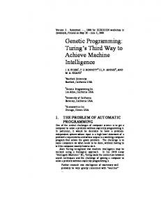
600
700
Avg size vs. time, different target size functions
400
Local 300
Average size
500
Linear
100
200
Limited
Sin
Constant 0
Nic McPhee (U of Minnesota, Morris)
100
200 300 400 Generation 6 Mux, Pop size 2000, c * size penalty
Bloat control in GP
500
13 June 2008, U of Granada
20 / 21
Dynamically computing parsimony penalty
Empirical results
Thanks!
Thanks for your time and attention! Thanks also to J.J. Merelo for inviting me out to the University of Granada. Contact:
[email protected] http://www.morris.umn.edu/~mcphee/ Questions?
Nic McPhee (U of Minnesota, Morris)
Bloat control in GP
13 June 2008, U of Granada
21 / 21