numeric intervals', 3rd International Workshop on Software Engineering, Ar- ti cial Intelligence and Expert Systems, Oberammergau, 1993. 6] C. K. Chiu and ...
Boosting the Interval Narrowing Algorithm Olivier Lhomme
E� cole des Mines de Nantes 4, rue Alfred Kastler, La Chantrerie, 44070 Nantes Cedex 03, France
Arnaud Gotlieb
Dassault Electronique and Universit�e de Nice { Sophia Antipolis
Michel Rueher
Universit�e de Nice { Sophia Antipolis I3S-CNRS Route des colles, BP 145, 06903 Sophia Antipolis, France
Patrick Taillibert
Dassault Electronique 55, Quai Marcel Dassault 92214 Saint-Cloud, France
Abstract Interval narrowing techniques are a key issue for handling constraints over real numbers in the logic programming framework. However, the standard xed-point algorithm used for interval narrowing may give rise to cyclic phenomena and hence to problems of slow convergence. Analysis of these cyclic phenomena shows: 1) that a large number of operations carried out during a cycle are unnecessary; 2) that many others could be removed from cycles and performed only once when these cycles have been processed. What is proposed here is a revised interval narrowing algorithm for identifying and simplifying such cyclic phenomena dynamically. First experimental results show that this approach improves performance signi cantly.
1 Introduction Interval narrowing techniques allow a safe approximation of the set of values that satisfy an arbitrary constraint system to be computed. Lee and Van Emden [13] have shown that the logic programming framework can be extended with relational interval arithmetic in such a way that its logic semantics is preserved, i.e., answers are logical consequences of declarative logic programs, even when oating-point computations have been used. These reasons have motivated the development of numerous CLP systems based on interval arithmetic (e.g., BNR-Prolog [20], Newton [1], CLP(BNR) [3], Interlog [12, 5, 14], Prolog IV [4]). All these systems use an arc consistency like algorithm [17] adapted for numeric constraints [8, 7].
The standard interval narrowing algorithm has two main limitations : � the so-called problem of early quiescence [8], i.e., the algorithm stops before reaching a good approximation of the set of possible values. This problem is due to the fact that interval narrowing algorithm guarantees only a partial consistency; � the problem of the existence of slow convergences, leading to impossibly long response times for certain constraint systems. Unlike the rst problem, for which many algorithms have been proposed [11, 14, 10, 9, 1, 6], the second problem has never been studied in the literature. This paper addresses this second problem. It shows that there is a strong connection between the existence of cyclic phenomena and slow convergence. The aim is to identify cyclic slow convergence phenomena while executing the interval narrowing algorithm and then to simplify them in order to improve performance.
1.1 Motivating example
The interval narrowing algorithm works iteratively: constraints are used for reducing domains until a xed point is reached. Experimental running times of this algorithm are generally well below the upper bound of the running time as given by a theoretical analysis (i.e., O(ma) where m is the number of constraints and a the size of the largest domain). However, slow | or asymptotic | convergence phenomena sometimes occur, and then the experimental running time approaches the theoretical bound, as in the example described in gure 1. = (a) Y = 1:001 � X (b) Y = 2�X (c) (e) = (d) Z2 = eZ1 = [0 10] DY = (?1; +1) DZ1 = (?1; +1) DZ2 = (?1; +1)
Y X Z1 eY DX ;
(a) & DX = [0; 10] ?! DY = [0; 10] (c) & DY = [0; 10] ?! DX = [0; 5] (e) & DZ1 = [1; e10] ?! DZ2 = [e; ee10 ] (b) & DY = [0; 5] ?! DX = [0; 4:99] (d) & DY = [0; 5] ?! DZ1 = [1; e5] etc.
(b) & DY = [0; 10] ?! DX = [0; 9:99] (d) & DY = [0; 10] ?! DZ1 = [1; e10] (a) & DX = [0; 5] ?! DY = [0; 5] (c) & DY = [0; 5] ?! DX = [0; 2:5] 5 (e) & DZ1 = [1; e5] ?! DZ2 = [e; ee ]
Figure 1: A slow convergence phenomenon Intuitively these phenomena are cyclic. In the above case the cycle is made up of the ve constraints (a; b; c; d; e). However, the reduction of DX induced by constraint (c) is stronger than the reduction of DX induced by constraint (b), so there is no point in applying constraint (b). Only (a), (c), (d) and (e) are relevant and the cycle could be simpli ed to (a; c; d; e). Constraints (d) and (e) only intervene in the cycle to reduce the domains of Z1 and Z2. It would be better to defer applying constraints (d) and (e). The
cycle would thus be simpli ed to (a; c) and constraints (d; e) would only be applied once the xed point has been reached. The number of computations carried out by the interval narrowing algorithm at each step would hence be minimized. The presence of a cycle implies the existence of a series uk = f (uk?1 ) which converges towards a xed point u such that u = f (u). The equation x = f (x) could be solved by a computer algebra system. In the above example, constraints (a) and (b) are linear and can be solved symbolically. However, a symbolic solution cannot be computed for arbitrary systems of constraints. The equation x = f (x) could also be solved by numeric methods. In particular, methods from interval analysis [19] have the same nice property as interval narrowing: a safe approximation of the set of solutions can be computed. However it is unclear how such methods can be generalized to non-square systems. Thus the aim of this research is to simplify the equation x = f (x) in order to accelerate convergence towards the xed point u. Two types of cycle simpli cations are proposed: removing the non-relevant narrowing functions and postponing some other ones. More precisely, given a cyclic phenomenon (a; b; c; d; e) such that: � b performs a weaker reduction than c, � d and e could be processed only once at the end of cycle, the goal is to replace n iterations of (a; b; c; d; e) by n iterations of (a; c) followed by one iteration of (d; e).
1.2 Relevance of automatic cycle simpli cation
At rst sight, one could think that slow convergence phenomena do not occur very often. It is true that early quiescence of interval narrowing algorithm is far more frequent than slow convergence. However, when the interval narrowing algorithm ends prematurely, a kind of enumeration interleaved with this algorithm is generally performed (e.g. domain splitting [7] or stronger consistencies [14]). During this interleaved process, slow convergence phenomena have a great chance to occur and to increase the required computing time considerably. Slow convergence phenomena move very often into cyclic phenomena after a transient period (a kind of stabilization step). For linear systems of constraints, slow convergence always entails a cyclic phenomenon. Of course, in this case the slow convergence phenomenon can be removed by simplifying the linear system with a linear solver. Cooperation between the interval narrowing solver and a linear solver is especially worthwhile in this latter case [6, 22, 18]. For arbitrary non-linear systems, slow convergence very often leads to a cyclic phenomenon. As arbitrary non-linear systems cannot be tackled with a symbolic solver, automatic cycle simpli cation is the only way to accelerate convergence in the majority of real applications.
1.3 Organization of the paper
Section 2 introduces some basic de nitions. In section 3, the concept of propagation cycle is introduced. This section shows that the standard interval narrowing algorithm will not allow cyclic phenomena to be satisfactorily simpli ed. Thus, a revised interval narrowing algorithm is proposed in which cyclic phenomena can be signi cantly simpli ed. Such a simpli cation of a cycle is proposed in section 4. In section 5, rst experimental results are provided. Finally, in section 6, the limits of such an approach are discussed.
2 Interval narrowing
2.1 Basic notations and de nitions
� IF denotes the set of oating-point numbers augmented with the two symbols f?1; +1g which represents respectively all numbers smaller
(resp. greater) than the smallest (resp. the biggest) oating-point number; � I (IF ) denotes the set of intervals [a; b] where a; b 2 IF ; ! � A CSP [17] is a!triple (X ; D; C ) where X = fx1; : : : ; xng denotes a set of variables, D= (D1; : : : ; Dn) denotes a vector of domains, Di the ! ith component of D being the domain of xi , and C = fC1; : : : ; Cmg denotes a set of constraints. This paper concentrates only on CSPs whose domains are intervals ! over the oating-point numbers, i.e., D 2 I (IF )n [8, 11, 14, 10, 1]; � A k-ary constraint C is a relation over the reals (i.e. a subset of IRk ). appx(C ) denotes the smallest (w.r.t. inclusion) subset of I (IF )k which contains C (we consider as in [13, 1] that results of oatingpoints operations are outward-rounded to preserve correctness of the computation).
2.2 Narrowing functions
The interval narrowing algorithm uses an approximation of the unary projection of the constraints to reduce the domains of the variables. Let C be a k-ary constraint over (xi1 ; : : : ; xi ), and (I1; : : : ; Ik ) 2 I (IF )k : for each j in 1::k, �i (C; I1 � : : : � Ik ) denotes the projection of appx(C ) on xi in the part of the space delimited by I1 � : : : � Ik , i.e., �i (C; I1 � : : : � Ik ) = faj j 9(a1 ; : : : ; ak ) 2 appx(C ) \ I1 � : : : � Ik g APi (C; I1 � : : : � Ik ) denotes an approximation of the projection of a constraint equal to the smallest interval encompassing the projection: [inf �i (C; I1 � : : : � Ik ); sup �i (C; I1 � : : : � Ik )] Such an approximation1 is computed by the evaluation of what will be called a narrowing function. For convenience, a narrowing function will be considk
j
j
j
ered as a ltering operator over all the domains, i.e, from I (IF )n to I (IF )n . For a k-ary constraint C over (xi1 ; : : : ; xi ) there are k narrowing functions, one for each xi where i 2 fi1; : : : ; ik g. The narrowing function of C over the ! ! variable xi is the function f : I (IF )n ?! I (IF )n de ned as f (D ) =D0 such that : � Di0 = APi(C; Di1 � : : : � Di ) ; � j 2 f1; :::; ng; i 6= j =) Dj0 = Dj (except the ith domain, all domains ! ! of D0 and D are identical) A narrowing function f may reduce the domain of only one variable (xi in the above de nition), called left-variable of f and denoted f:y . The constraint from which the function f is issued is denoted f:c and the set of variables whose domains are required for the evaluation of the domain of f:y is called right-variables set and is denoted f:xs . Properties 2.1. The three following properties trivially hold: ! ! � f (D ) � D ! ! � f (f (D)) = f (D) � if f and g are narrowing functions of the same constraint (i.e, g:c = ! ! f:c) then f (g(f (D))) = g(f (D)) ! In this paper, a numeric CSP (X ; D; C ) will also be denoted by a triple ! (X ; D; F ) where F is the set of narrowing functions corresponding to the constraints in C . Figure 2 shows such a view of a CSP (�j (C ) denotes the narrowing function of C over the variable xj ; thus f = �1 (a) reduces D1 based on D2). k
k
!
Let < X ; D; C > be a CSP where C = fa; bg: (a) x1 ? x2 + 3 = 0 (b) x3 = x1 ! This CSP can be formulated in the form < X ; D; F > where F = ff; g; h; ig f = �1(a) h = �2(a) i = �1 (b) g = �3(b) !
Figure 2: A CSP in the form < X ; D; F > Using the above notations, the standard interval narrowing algorithm [8, 7] can be written as in gure 3. In the rest of this paper, a set of narrowing functions T will be associated to a � ltering operator T that computes the intersection of the� domains narrowed ! by the functions in T : Let T = ff1 : : : ; fpg � F , T (D) is de ned by ! ! � ! ! f1(D) \ : : : \ fp (D). If T = ; then by convention T (D) =D . ! Just note that if! D0 is !the xed point reached by the interval narrowing � algorithm then D0 =F (D0 ).
IN-1(in F , inout D!) Queue F ; while Queue =6 ;
!
!
POP Queue; D0 f (D ); !0 ! ! if D 6= D then !D D0; Queue Queue [ fg 2 F j g:c 6= f:c and f:y 2 g:xs g
f
endif endwhile
Figure 3: Interval narrowing algorithm
3 Towards a characterization of the cyclic phenomenon When the interval narrowing algorithm runs into a slow convergence phenomenon a cyclic phenomenon may occur after a transient period. In this section, we give a precise de nition of a cyclic phenomenon. Further de nitions are now required to formalize such cyclic phenomena. Let us outline our approach in very general terms: (1) we show that information about some dynamic dependencies (in place of static ones) between narrowing functions is required; (2) such information about dynamic dependencies cannot be identi ed in the framework of the IN-1 algorithm. This is due to the fact that the order in which the narrowing functions are en-queued plays a major role in IN-1; (3) in order to get information about some dynamic dependencies we introduce a revised version of the IN-1 algorithm.
3.1 Static dependency
A static dependency between two narrowing functions f and g | denoted by f !s g | means that after an evaluation of f which modi es the domain of f:y , g may reduce the domain of g:y (the narrowing functions en-queued in interval narrowing algorithm are the ones which statically depend on f ). s De nition 3.1. (static dependency) A static dependency f ! g holds i�: � g:c 6= f:c (f and g are functions not issued from the same constraint) � f:y 2 g:xs (the left-variable of f occurs in the right-variables set of g) We note succs (T ) the successors in the static dependency sgraph of a set of narrowing functions T : succs (T ) = fg 2 F j 9f 2 T ^ f ! g g. Static dependency information may not be su�cient for cycle simpli cation. ! For instance, consider the example in gure 2: f !s g , i.e., g (f (D)) may ! ! ! be di�erent from f (D ). However, let D0 = f (D) and suppose that D30 is ! ! included in D10 , then g (f (D)) = f (D ). Such an equality would allow g to be
removed from a possible cycle; unfortunately, f !s g does not allow to infer this equality and thus no cycle simpli cation can be performed in this case. d What is needed is a dynamic dependency f ! g that ensures that a modi cation induced by f actually implies a modi cation induced by g . The rst idea is to follow interval narrowing algorithm and try to identify such dynamic dependencies.
3.2 Dynamic dependency
Algorithm IN-1 computes the terms of a sequence of ith term fi (fi?1 (::: ! f0(D))) characterizing the order in which the narrowing functions fj are en! queued: fi (fi?1 (:::f0(D))) corresponds to the en-queueing order (f0 ; f1; :::;s fi). Let us assume that! a dynamic dependency holds between f and g if f ! g ! and g (f (D)) 6= f (D). Such a de nition would lead to several problems: ! (1) g (f (D)) is not always computed by algorithm IN-1 since some narrowing functions may have been! en-queued between f and g , e.g., IN-1 may compute g (h1(:::(hk(f (D))))). ! ! (2) The fact that f !s g and g (f (D)) 6= f (D) does not always imply ! an e�ective dynamic dependency between f and g since g (D) could ! ! already be di�erent from D . For instance, if g (f (h1(:::(hk (D0 ))))) is computed, then the e�ective dynamic dependency may hold between hj and g. (3) The narrowing functions from which g dynamically depends may be dynamically dependent between themselves, meaning that the dependencies are interleaved.
Example! Let < X ; D ; F > be a CSP where : � F = ff; g; hg � D4 = [0; 2�]. � f = �1 (x1 = x9 ) � g = �2 (x2 = x1) � h = �3(x3 = x2 + cos(x4 + x1)) ! Suppose that h(g(f (D ))) is computed!(according to en-queueing order of the narrowing! functions). Suppose also that! D veri es: ! ! ! ! � g(D)!= D and!h(D ) = D, � f (D ) = 6 !D, ! � g(f (D )) = 6 f (D ), � h(g(f (D ))) = 6 g(f (D )). That is f , g and h perform a reduction. The static dependencies are: f !s g; f !s s d d h; g ! h. According to the above naive de nition, f ! h and g ! h hold. However
actually depends only on g (the reduction of D3 is only due to the modi cation of D2 computed by g). h
Identifying dynamic dependencies which allow optimal cycle simpli cations would require considering a great number of permutations of narrowing functions in the queue, and thus, would be far too expensive to be computed. What is proposed here is a de nition of the dynamic dependencies such that: � most of the cycles can be reduced signi cantly,
� the set of dynamic dependencies can be computed in an e�cient way.! A dynamic dependency is parameterized by the domains of the variables D and by a set of narrowing functions T (whose meaning will be made clear in the next subsection). De nition 3.2. (dynamic dependency) ! d(T ;D ) A dynamic dependency f ?! g holds i� � f 2 T , f !s g, � ! � ! � g(T (D)) 6=T (D) (intuitively g reduces a domain due to a narrowing function in T ).
3.3 Revised algorithm for interval narrowing
We reformulate the interval narrowing algorithm such that the dynamic dependencies can be computed in an e�cient way. The revised version (Figure ! 4) applies on the same vector D all the narrowing functions which may reduce a domain. This will make it possible to nd the dynamic dependencies. The xed point towards which the revised algorithm2 converges is identical ! � ! 0 to that of the standard algorithm (i.e., a domain vector D such that F (D0) ! =D0 ).
Revised-IN-1(in F , inout D!) T F; while !T =6 ; ! ! � ! D0 D; D T (D); � ff 2 T j Di0 = 6 Di and f:y = xig; T succs (� ); Figure 4: Revised interval narrowing algorithm The revised interval narrowing algorithm computes the terms of a sequence � � � ! th of n term T n (T n?1 (: : : (T 0 (D0)))) where ! ! � D0=D, T0 = F , � � Ti =! succs(ff 2 Ti?1 j f:y = xj and Dj has been reduced by T ! � � ! i?1 g). th Let also Di be the domain vector at the i step: D i = T i?1 (:::T 0 (D0)). � ! � ! � � ! � i+1 ! Of course, T i (Di ) = F (Di ) and so T i (:::T 0(D0 )) = F (D0).
3.4 Relevant narrowing functions
As outlined in the introduction, when two narrowing functions perform a reduction of the same domain of the variables, it is possible to remove the narrowing function which performs the weakest reduction of the domain.
The relevant narrowing functions are the one which perform the strongest reductions� of the domains of the variables during the application of the operator T . The domains being intervals, there may be 0, 1 or 2 (one for the lower bound, one for the upper bound) relevant narrowing functions for each variable. Let Ri be the set of those relevant narrowing functions. De nition 3.3. (relevant narrowing functions) � ! � ! � ! Ri � Ti is a minimal3 subset of Ti such that Ri (Di) =T i (Di) = F (Di). � Computing Ri only consists | when applying T i in Revised-IN-1 | in keeping, for each bound of a domain, the narrowing function that leads to the strongest reduction. In a cyclic phenomenon, the relevant narrowing� functions will be a� priori ! ! known and then it will be su�cient to compute Ri (Di ) in place of T i (Di ).
3.5 Computing the dynamic dependencies
As the non-relevant narrowing functions will be removed from the cycle, the dynamic dependencies have to be computed only for the relevant narrowing functions. Let G be the dynamic! dependency graph. The dynamic dependencies are functions of Ri and Di . The vertices are some pairs < f; i > where f is a narrowing function and i is the index of the inference step. An arc from ! < f; i > to < g; i + 1 > will represent a dynamic dependency f d(R?!;D ) g. Let Gi be the subgraph of G which is only concerned with the ith step of the algorithm. Gi is a bipartite graph from < Ri ; i > to < Ri+1 ; i + 1 >. A function g in Ri+1 being relevant it performs a reduction of a domain. s Thus there is an arc from < f; i > to < g; i + 1 > i� f ! g . Then, the set of dynamic dependencies represented by Gi is the subset of the static dependencies whose starting functions are in Ri and the ending ones are in Ri+1. The dynamic dependency graph G is just the union of its subgraphs Gi at the di�erent steps. An example of a dynamic dependency graph is given in gure 5 (a). i
i
< f1 ; 0 >
< f2 ; 1 >
< f5 ; 2 >
< f1 ; ^0 >
< f2 ; ^1 >
< f5 ; ^2 >
< f2 ; 0 >
< f3 ; 1 >
< f6 ; 2 >
< f2 ; ^0 >
< f3 ; ^1 >
< f6 ; ^2 >
(a)
< f4 ; 1 >
(b)
< f4 ; ^1 >
Figure 5: Dynamic dependency graphs
3.6 De nition of a cyclic phenomenon
A propagation cycle formalizes a cyclic phenomenon: ! De nition 3.4. A propagation cycle is a quintuple < X ; D; F ; p; ArrayR > where: ! � < X ; D; F > is a CSP; jFj = m; ! ! � 9N >> m; F N (D) 6= F N ?1(D) i.e, a slow convergence4 occurs; � p is the period of the cycle; � let Ri be the relevant narrowing functions at the step i, then 8i < N; Ri+p = Ri ,i.e., the sets of relevant narrowing functions re-occurs periodically; � ArrayR[i mod p] = Ri (the relevant narrowing functions are kept in ArrayR). A propagation cycle of period 3 means that the subgraph Gi is equal to the subgraph Gi mod 3 ; thus the dynamic dependency graph is cyclic (see gure 5 (b) where ^0 denotes all the steps i such that i mod 3 = 0).
4 Simplifying a cycle
4.1 Pruning the dynamic dependency graph
Two types of simpli cations were mentioned in the introduction: (1) Removing the non-relevant narrowing functions; (2) Postponing some narrowing functions. The rst one is now interleaved with the cycle de nition (where the Ri sets have to be known). The second one can now be formulated easily: a vertex < f; i > which does not have any successor in the dynamic dependency graph corresponds to a narrowing function that can be postponed. Such a vertex can be removed from the dynamic dependency graph. Applying this recursively will remove all the non-cyclic paths from the graph. For instance, in the graph (b) of the gure 5, the white arrows will be pruned. When a vertex is removed, the corresponding narrowing function is pushed onto a stack (the removing order must be preserved). Let R0i � Ri be the sets of narrowing functions whose corresponding vertices have not been removed from the graph, let s1 ; s2 ; :::; sl be the stacked narrowing functions (s1 being the rst stacked one); then it can be shown that � � � ! � � � ! �i ! s1(s2(:::sl(R0i (R0i?1 (::: R00 (D0 )))))) =Ri (Ri?1 (::: R0 (D0 )))) = F (D0 )
4.2
IN-2
algorithm
The algorithm proposed for cycle simpli cation is called IN-2. IN-2 operates in 4 steps: (1) observe the dynamic behavior and try to detect a cycle;
(2) simplify the detected cycle and stack the narrowing functions corresponding to a removed vertex in the dynamic dependency graph; (3) iterate on the simpli ed cycle until a xed point is reached; (4) when the xed point has been reached, evaluate the stacked narrowing functions. Step 1 boils down to running the IN-1 and observing that it continues to iterate after k iterations where k depends on the number of variables and the number of constraints of the problem. Henceforth the existence of a propagation cycle is assumed. Then Revised-IN-1 is started for nding the period of the propagation cycle and building ArrayR. To the authors-knowledge, there exists no e�cient algorithm for nding the period of the propagation cycle for the general case. However, it is always possible to nd the period of a sub-cycle. A history of the relevant narrowing functions just needs to be kept: when ArrayR[k] is built, ArrayR[k] and ArrayR[0] need to be compared (implementation is a little more complex since a stabilization step has to be performed). If they are equal, we have a candidate that could be a sub-cycle of period p = k. It is then possible to verify that it is repeated during the following k steps. It is di�cult to be sure that this sub-cycle is the propagation cycle as it could just be a cycle within the actual propagation cycle. Be this as it may, in most cases it is acceptable to take the rst sub-cycle to be encountered. Step 2 has been described in section 4.1. An upper bound of the running time for simplifying the cycle is O(v ) where v is the number of vertices in the dynamic dependency graph. Note that in examples built for this special purpose v could be a very large number. However, v is generally of the same order of magnitude as m, the number of narrowing functions. The rst step of the algorithm can take into account an upper bound for the number of vertices in the sub-cycle. � � � ! Step 3 consists in computing R0i (R0i?1 (::: R00 (D0 ))), using the fact that R0i = ArrayR[i mod p]: An upper bound of the running time of this iteration procedure is O(a � m0) where m0 is the number of di�erent narrowing functions occurring in ArrayR and a is the maximum size of the domain of the variables (note that a is here a very large number). Since the existence of a propagation cycle leads to a phenomenon of slow convergence it is reasonable to suppose that the other parts of the general algorithm represent but a tiny part of the computation time, and O(a � m0) can be compared with the complexity of the standard interval narrowing algorithm: O(a � m) where m is the total number of narrowing functions[16, 23, 14]. Step 4 evaluates the relevant narrowing functions corresponding to the removed vertices when the xed point of the interval narrowing algorithm has been reached. This must be done in reverse order to their removal. This procedure is in O(l) where l is the number of the removed vertices.
Problem 1 2 3 4
Table 1: List of Examples System of Constraints x1 = sin(x2 ) x2 = x1 x1 = sin(x2 ) x3 = x1 � x2 x2 = x1 x1 = sin(x2 ) x3 = exp(x1) x4 = exp(x3) x2 = x1 x1 = sin(x2 ) x3 = exp(x1) x4 = exp(x3) x5 = 3 � x4 x6 = exp(x4 ) x7 = x6 x8 = 5 � x7 x9 = x7 x10 = 4 � x9 x2 = x1
Table 2: Computation Results Problem Postponed narrowing functions Improvement rate 1 0 3:4 2 1 6:2 3 2 12 4 8 32:3
5 Implementation & experimental results The IN-2 algorithm has been implemented and integrated in Interlog [12, 15], a CLP(Intervals) system. The standard interval narrowing algorithm is always restarted after the four steps of IN-2 in order to make sure that the same xed point is computed. The examples in Table 1 only di�er by an increasing number of narrowing functions that can be postponed. Table 2 reports the improvement factor gained with dynamic cycle simpli cation. Improvement rate represents the ratio t1 =t2 where t1 is the running time of the standard interval narrowing IN-1 and t2 is the running time of the revised interval narrowing with cycle simpli cation IN-2. Note that even for a problem without any cycle simpli cation ( rst problem) the improvement factor is more than 3 times. This is only due to the fact that the en-queueing/de-queueing operations are no longer performed.
6 Discussion First of all, let us not forget that the algorithm suggested here does not detect a propagation cycle but a sub-cycle. Although, in the vast majority of cases, this sub-cycle corresponds to the cycle, this is not always the case. One way of tackling this problem is simply to interrupt the iteration in the IN-2 algorithm after a certain number of iterations (but before reaching the xed point), then to run the algorithm again from step 1. This approach o�ers two further advantages: � In an over-constrained problem (which has no solution) the removed vertices may possibly detect a contradiction. It may therefore be useful
to periodically re-apply the narrowing functions corresponding to the removed vertices before reaching the xed point. � Secondly, so far the working hypothesis has been that there is a cyclic phenomenon. In fact, when a phenomenon of slow convergence happens in the interval narrowing algorithm it is usually, but not always a single cyclic. As a general rule a phenomenon of slow convergence can be decomposed into a series of cyclic steps separated by a transient, acyclic one. By periodically reinitializing the cycle detection process it should be possible to detect a new cycle and to simplify it. Using a language where meta-evaluation is authorized, before iteration it is possible to transform the table ArrayR into explicit code and thus the cycle would really be compiled. The revised model of the interval narrowing algorithm applies the narrowing functions on the same domain vector whereas in the standard interval narrowing algorithm they are applied sequentially. Once a propagation cycle has been detected and simpli ed, it is possible to use a sequential iteration procedure (closer to the standard algorithm). Let ArrayR[k] be the set ff1; :::; fqg, the iteration procedure (step 3) can apply ! ! f1 (:::fq (D)) instead of T (D) where T = ArrayR[k]. This leads to another cyclic phenomenon, which could be itself optimized. The order in which the narrowing functions are evaluated can in uence this cyclic phenomenon. However, it seems di�cult to nd an order that is \better" than all the others. Dynamic cycle simpli cation is not based upon a speci c kind of narrowing functions but on the xed point algorithm which is used in almost all interval narrowing systems. The approach could then be combined with some recent advances in the eld like [1] and [10], which propose other narrowing functions. A related work is [24]. Although the problems of cycle detection are quite similar, the aim is not to optimize an algorithm but to generate an abstraction of repeating cycles of processes to perform more powerful reasoning in causal simulation.
7 Conclusion This paper proposes a method for greatly accelerating the convergence of the cyclic phenomena in the interval narrowing algorithm. The rst step requires simplifying this cyclic phenomenon by keeping just the relevant narrowing functions (i.e., the narrowing functions that actually perform the task). The second step consist in removing from the cycle those relevant narrowing functions that may be deferred. In this way it is possible to reduce the theoretical upper bound of the running time from O(am) to O(am0 ), where m is the total number of narrowing functions, m0 is the number of relevant narrowing functions occurring in the cycle and a is the maximum size of the domains of the variables.
In order to enable the simpli cation of the propagation cycles, a revised interval narrowing algorithm has been introduced. First experimental results indicate that an automatic cycle simpli cation can produce signi cant improvements in e�ciency over standard interval narrowing.
Acknowledgements Thanks to Christian Bliek, Patrice Boizumault, Bernard Botella, Helene Collavizza, Narendra Jussien, Emmanuel Kounalis, Philippe Marti, Peter Sander, Serge Varennes, Dan Vlasie and the reviewers for their helpful comments.
Notes 1 For most non-linear constraint systems, AP (C ; I1 � : : : � I ) cannot be computed in a i
p
k
straightforward way. However, interval arithmetic [19] allows it to be computed on a subset of the constraints set, called basic constraints. Each constraint can be approximated by decomposition in basic constraints [14]. For instance, let C be the constraint x1 ?x2 +3 = 0, AP1 (C; I1 � I2 ) can be expressed by I1 \ (I2 ? 3) using interval arithmetic. Any other approximation of the projection (e.g. [1]) could have been taken in place of this one. 2 The theoretical complexity of the revised version is higher than that of the standard algorithm. However this algorithm will not be used for computing the xed point but only for catching the dynamic dependencies. For information, an upper bound of the running time is in O(n � m � a) instead of O(m � a) where m is the number of constraints, n is the number of variables and a the size of the largest domain. 3 If two narrowing functions perform the same reduction on the same bounds, only the rst one according to a lexical order is considered as relevant. 4 The speed of convergence is a relative notion. The revised algorithm is said to ! converge slowly for (X ; D; F ) when the number of iterations required to reach the xed point is much greater than m (the number of narrowing functions of F ), i.e, when 9N >> ! ! m; 8k < N; F k+1 (D) 6= F k (D).
References [1] F. Benhamou, D. Mc Allester, and P. Van Hentenryck, `CLP(Intervals) Revisited', in Proc. Logic Programming: Proceedings of the 1994 International Symposium,MIT Press, (1994). [2] F. Benhamou, `Interval Constraint Logic Programming', in in [21] [3] F. Benhamou and W. Older, `Applying interval arithmetic to real, integer and boolean constraints', Journal of Logic Programming, (1994). [4] A. Colmerauer, `Sp�eci cations de Prolog IV', Draft, 1994. [5] B. Botella and P. Taillibert, `INTERLOG : constraint logic programming on numeric intervals', 3rd International Workshop on Software Engineering, Arti cial Intelligence and Expert Systems, Oberammergau, 1993. [6] C. K. Chiu and J. H. M. Lee, `Towards Practical Interval Constraint Solving in Logic Programming', in ILPS'94: Proceedings 11th International Logic Programming Symposium, (Ithaca), (1994).
[7] J. Cleary, `Logical arithmetic,' Future Computing Systems, vol. 2, no. 2, pp. 125{149, 1987. [8] E. Davis, `Constraint propagation with interval labels', Arti cial Intelligence, 32, 281{331, (1987). [9] D. Haroud and B. Faltings, `Global consistency for continuous constraints,' in PPCP'94: Second Workshop on Principles and Practice of Constraint Programming (A. Borning, ed.), (Seattle), May 1994. [10] B. Faltings, `Arc consistency for continuous variables,'Arti cial Intelligence, 65(2), 1994. [11] E. Hyv}onen, `Constraint reasoning based on interval arithmetic: the tolerance propagation appoach', Arti cial Intelligence, vol. 58, pp. 71{112, 1992. [12] Dassault Electronique, `INTERLOG 1.0 : Guide d'utilisation',DE, 55, quai Marcel Dassault, 92214 Saint Cloud, 1991. [13] J. H. M. Lee and M. H. van Emden, `Interval computation as deduction in CHIP', Journal of Logic Programming, 16:3{4, pp.255{276, 1993. [14] O. Lhomme, `Consistency techniques for numeric CSPs', in Proc. IJCAI93, Chambery, (France), pp. 232{238, (August 1993). [15] O. Lhomme, `Contribution �a la r�esolution de contraintes sur les r�eels par propagation d'intervalles', PhD dissertation, 1994. Universit�e de Nice | Sophia Antipolis BP 145 06903 Sophia Antipolis [16] A. Mackworth and E. Freuder, `The complexity of some polynomial network consistency algorithms for constraint satisfaction problems,' Arti cial Intelligence, vol. 25, pp. 65{73, 1985. [17] A. Mackworth, \Consistency in networks of relations," Arti cial Intelligence, vol. 8, no. 1, pp. 99{118, 1977. [18] P. Marti and M. Rueher, `A distributed cooperating constraints solving system', Special issue of IJAIT (International Journal on Arti cial Intelligence Tools), 4(1-2), 93{113, (June 1995). [19] R. Moore, Interval Analysis. Prentice Hall, 1966. [20] W. Older and A. Vellino, `Constraint arithmetic on real intervals', in Constraint Logic Programming: Selected Research, eds., Fr�ed�eric Benhamou and Alain Colmerauer. MIT Press, (1993). [21] Andreas Podelski,Constraint Programming: Basics and Trends, LNCS 910, 231{250, Springer Verlag (1995). (Ch^atillon-sur-Seine Spring School, France, May 1994). [22] M. Rueher, `An Architecture for Cooperating Constraint Solvers on Reals', in [21] [23] P. Van Hentenryck, Yves Deville, and Choh-Man Teng. A generic arcconsistency algorithm and its specializations. Arti cial Intelligence, 57(2{ 3):291{321, October 1992. [24] D. S. Weld, `The use of aggregation in causal simulation,' Arti cial Intelligence, vol. 30, pp. 1{34, 1986.