ABSTRACT. We present a generalized sequential probability ratio test for com- posite hypotheses wherein the thresholds are updated in an adaptive manner ...
BOOTSTRAP BASED SEQUENTIAL PROBABILITY RATIO TESTS Fiky Y. Suratman and Abdelhak M. Zoubir Signal Processing Group,Technische Universit¨at Darmstadt Merckstrasse 25, 64283, Darmstadt, Germany ABSTRACT We present a generalized sequential probability ratio test for composite hypotheses wherein the thresholds are updated in an adaptive manner based on the data recorded up to the current sample using the parametric bootstrap. The resulting test avoids the asymptotic assumption usually made in earlier works. The increase of the average sample number of the proposed method is not significant compared to the sequential probability ratio test which is based on known parameters, especially in a low SNR region. In addition, the probability of false alarm and the probability of missed detection are maintained below the preset values. A comparison shows that the thresholds based on the parametric bootstrap are in close agreement with the thresholds based on Monte-Carlo simulations. Index Terms— Bootstrap, sequential probability ratio test, composite hypothesis, spectrum sensing, cognitive radio 1. INTRODUCTION The sequential probability ratio test (SPRT) was pioneered by Abraham Wald in 1943 in a confidential report, which was then published in 1945 [1]. His initial work on the general theory of the cumulative sum [2] has provided a tool to derive the operating characteristic and the average sample number as the performance indices of the SPRT. The main idea behind the SPRT is to pre-specify the probability of detection errors (false alarm and missed detection) and minimize the average of required sample number [1, 3]. This scheme results in a random sample number with its average smaller than the corresponding best fixed sample number detector. The work of Bussgang and Middleton [4] applies Wald’s SPRT to sequentially detect signals in noise. The case of correlated observation is also treated. Subsequently, some analytical results and modified procedures on the SPRT also have been introduced, such as in [5–7]. In addition, since the SPRT has an average sample number (ASN) larger than the corresponding fixed sample number detector when the parameter value lies between the two simple hypotheses, some methods to reduce the sample number in this condition have been proposed [8,9]. They are known as truncated SPRT. Implementation of sequential analysis to a distributed environment can be found, for example, in [10, 11]. Recently, the superiority of the sequential detector in reducing the sample number is an attractive choice in spectrum sensing for cognitive radio (CR) [12]. This is because a short duration of sensing time (a small sample number) is required in spectrum sensing to improve agility of the CR users, which successively increase the throughput of a CR network and reduce the degree of interference to the licensed network. Some examples of the implementation in this emerging research field are [13–17]. However, addressing sequential detections for composite hypotheses is only few in literature. The bootstrap, a computer-based method for assigning measures of accuracy to statistical estimates [18], is used here. From a data
978-1-4799-0356-6/13/$31.00 ©2013 IEEE
6352
manipulation point of view, the main idea encapsulated by the bootstrap is to simulate as much of the real world probability mechanism as possible, in which any unknowns are replaced with estimates from the observed data. The application of the bootsrap to various signal processing techniques can be found in [19, 20] and references therein. In addition, bootstrap-based detection methods have been successfuly implemented in [21–23]. However, the literature on bootstrapping methods for sequential detections is very scarce. Some studies in [24, 25] on sequential detection for composite hypotheses have focused on asymptotic optimality and properties for the general non-iid case. In this setup, the probability of false alarm and the probability of missed detection are assumed to converge to zero or the constant thresholds are assumed to converge to infinity. The present work, in some sense, is based on the same framework as [16]. However, the authors in [16] mainly concentrate on finding a bound on the error term of the log-likelihood ratio in the asymptotic sense, such that the threshold margin for the upper and the lower thersholds, which are functions of the sample number, can be replaced by some positive constants. Eventually, constant thresholds are used in this earlier work. In general, the present paper differs from the previous work in several aspects. First, the SPRT is extended to cope with the composite hypothesis problem by combining the generalized SPRT and the parametric bootstrap to find the thresholds. Second, the thresholds are not constant but updated for each new sample recorded and also suitable for small sample number, not only in the asymptotic sense. Hence, a smaller average sample number is possible. Last, exhaustive simulations to determine the thresholds in worst case scenario such as in [16] are avoided. The remainder of the paper is organized as follows. The SPRT for simple hypothesis is briefly explained in Section 2. Section 3 begins with signal model and discusses subsequently in detail the generalized SPRT and the proposed bootstrap based SPRT for composite hypothesis. An example and simulation results are presented in Section 4. Finally, the paper is concluded with Section 5. 2. THE SIMPLE HYPOTHESIS CASE The sequential probability ratio test (SPRT) for binary hypothesis testing is designed based on simple hypothesis H0 against simple alternative H1 [1, 3]. Let f (~xN ) denotes the density function of a random column vector ~xN = [x(1) x(2) · · · x(N )]T which represents the iid observations of a signal up to the N th sample. The density function f0 (~xN ) under H0 and f1 (~xN ) under H1 are assumed to be exactly known. Then, the SPRT is optimum for minimizing the sample number for targeted probability of false alarm α and probability of missed detection β among other tests [3]. The required sample number is not determined in advance, but it is random, depending on the statistics of the current observation. The test stops when either the upper constant-threshold A or the lower B is crossed for the first
ICASSP 2013
time. In summary, the SPRT can be written as accept H1 ≥ A, f (~ x ) 1 N ≤ B, accept H0 , Z¯N = log f0 (~xN ) A < Z¯ < B, continue to observe N
where ZˆN is the GLR from (4). The upper threshold AN and the lower BN are functions of the sample number N , (7)
∆iN
For the preset probability of false alarm α and missed detection β that are much smaller than 1, the thresholds can be calculated from Wald’s approximation [3] 1 , B = log β, (2) α to guarantee that the actual probability of false alarm Pf ≤ α and missed detection Pm ≤ β. A = log
3. THE COMPOSITE HYPOTHESIS CASE The simple hypothesis approach is not suitable in most practical scenarios, since unknown parameters might exist which enforce to use non-exact distributions. Therefore, we aim at extending the SPRT to the composite hypothesis case. Suppose that the detector receives a signal that is distributed according to H0 : ~xN ∼ f0 (~xN ; θ0 ), θ0 ∈ Θ0 H1 : ~xN ∼ f1 (~xN ; θ1 ), θ1 ∈ Θ1
AN = A + ∆0N , BN = B − ∆1N ,
(1)
where A and B are determined from (2), and ≥ 0, i = 0, 1, is the modified value for the threshold at the N th stage under Hi . The determination of ∆iN will be elaborated in the following subsection. 3.2. The Bootstrap Based SPRT (B-SPRT) The log-likelihood ratio ZˆN in (6) can be considered as an estimate i of the log-likelihood ratio Z¯N in (1) under hypothesis Hi , i = 0, 1, ! (N) f1 (~xN ; θ¯1 ) f1 (~xN ; θˆ1 ) f0 (~xN ; θ0 ) ˆ H0 : ZN = log + log f0 (~xN ; θ0 ) f1 (~xN ; θ¯1 ) f0 (~xN ; θˆ0(N) ) 0 0 = Z¯N + ∆ZN ! (N) f1 (~xN ; θˆ1 ) f0 (~xN ; θ¯0 ) f1 (~xN ; θ1 ) + log H1 : ZˆN = log f1 (~xN ; θ1 ) f0 (~xN ; θˆ0(N) ) f0 (~xN ; θ¯0 ) 1 1 = Z¯N + ∆ZN , (8) i where ∆ZN is the error term under Hi , i = 0, 1. The MLEs
(3)
(N) P (N) P ¯ H0 : θˆ0 → − θ0 θˆ1 − → θ1 , θ0 ∈ Θ0 , θ¯1 ∈ Θ1
where θ0 and θ1 are the unknown parameters in the respective hypothesis, and Θ0 , Θ1 ⊂ Θ are disjoint parameter spaces, i.e. Θ0 ∩ Θ1 = ∅.
in which
3.1. The Generalized SPRT
θ¯i = arg min KL(fj (~xN ; θj )||fi (~xN ; θˇi )), i, j = 0, 1, i 6= j, (10)
(N) P (N) P ¯ → θ1 , θ¯0 ∈ Θ0 , θ1 ∈ Θ1 − θ0 θˆ1 − H1 : θˆ0 →
θˇi ∈Θi
Note that the two parameters θ0 and θ1 in (3) are unknown. Hence, we replace them by their maximum likelihood estimates (MLEs). As in the case of a fixed sample number detector [26], the generalized log-likelihood ratio (GLR) can then be written as (N)
f1 (~xN ; θˆ1 ) ZˆN = log (N) f0 (~xN ; θˆ0 )
(4)
and KL(fj ||fi ) denotes Kullback-Leibler distance between distriP butions fj and fi . Here − → denotes convergence in probability as N → ∞. At stopping time N = NT , the probability of false alarm Pf and missed detection Pm can then be written as Pf
=
0 ≥ A|H0 ) P (ZˆNT ≥ ANT , Z¯N T 0 < A|H0 ) +P (ZˆN ≥ AN , Z¯N
≤ ≤ =
0 0 < A|H0 ) P (Z¯N ≥ A|H0 ) + P (ZˆNT ≥ ANT , Z¯N T T α + ∆Pf (11) 1 ≤ B|H1 ) P (ZˆN ≤ BN , Z¯N
≤ ≤
1 > B|H1 ) +P (ZˆNT ≤ BNT , Z¯N T 1 1 ¯ ˆ > B|H1 ) P (ZNT ≤ B|H1 ) + P (ZNT ≤ BNT , Z¯N T β + ∆Pm . (12)
where
T
T
(N) θˆi
(9)
= arg max log (fi (~xN ; θi ))
(5)
θi ∈Θi
is the MLE assuming hypothesis Hi , i = 0, 1 is true. Meanwhile, subscript or superscript N is to indicate the data has been recorded up to the N th sample. Furthermore, the two thresholds of the SPRT (2) cannot be used directly in this setup. A threshold modification is required to compensate the estimation errors, introduced by the MLEs. Otherwise, it will lead to early terminations that increase the actual probability of false alarm Pf and missed detection Pm . Note that we cannot just increase A or decrease B by some constants to improve Pf and Pm , since it will successively increase the average sample number. Meanwhile, the average of estimation errors is large for a small N and vice versa. Hence, to reflect this condition, an appropriate method is needed to set the thresholds adaptively based on N . In this way, they should be large to tolerate large estimation errors for N small and converge to (2) as N increases. The generalized SPRT for composite hypotheses can now be defined as [16] accept H1 ≥ AN , ≤ BN , accept H0 , ZˆN (6) AN < ZˆN < BN , continue to observe
6353
Pm
T
T
T
T
Hence, we aim at minimizing ∆Pf and ∆Pm by finding appropriate values for ∆0N and ∆1N of (7), respectively. Note that the thresholds should be calculated at each N th stage since the stopping time NT is not known in advance. Therefore, let the last terms of (11) and (12) be expressed as functions of N 0 P (ZˆN ≥ AN , Z¯N < A|H0 ) 0 ≤ P (|ZˆN − Z¯N | ≥ AN − A|H0 )
P (ZˆN
0 = P (|∆ZN | ≥ ∆0N |H0 ) 1 ≤ BN , Z¯N > B|H1 ) 1 ≤ P (|ZˆN − Z¯N | ≥ B − BN |H1 ) 1 = P (|∆ZN | ≥ ∆1N |H1 ).
(13)
(14)
Now, suppose that the two probabilities are pre-specified as tolerance values to represent ∆Pf and ∆Pm 0 1 P (|∆ZN | ≥ ∆0N |H0 ) = ǫ0 , P (|∆ZN | ≥ ∆1N |H1 ) = ǫ1 .
(15)
Accordingly, ∆iN , i = 0, 1, can be found by using the parametric bootstrap of (15) to finally get (AN , BN ) in (7). In our setup, the thresholds at the (N + 1)th stage is calculated based on the observed data up to the N th sample. Hence, upon receiving the (N + 1)th sample, the log-likelihood ratio ZˆN+1 is computed and then compared to the calculated thresholds (AN+1 , BN+1 ). In principle, the parametric bootstrap replaces any unknown parameters with estimates and re-uses data to provide a way to approximate distributional information, using the measured sample as a basis. Suppose that N samples have been recorded and are represented by ~xN . Let Fθ be the distribution of ~xN , parameterized by θ. Bs bootstrap replications of size N + 1 are generated from parametric estimates of the population Fˆθˆ(N ) by assuming Hi i is true, i.e. 0b 0b T H0 : Fˆθˆ(N ) → ~x0b N+1 = [x1 · · · xN+1 ] 0
1b 1b T H1 : Fˆθˆ(N ) → ~x1b N+1 = [x1 · · · xN+1 ] , b = 1, · · · , Bs
(16)
1
(N) (N) parameterized by θˆ0 and θˆ1 which are the MLEs from (5). Note that we generate the bootstrap replications for H0 and H1 to get the upper threshold AN and the lower threshold BN , respectively. Furthermore, the log-likelihood ratios ZˆN+1 and Z¯N+1 are computed for all bootstrap replications b = 1, · · · , Bs of each assumed hypothesis,
ˆ(N+1)ib ) ¯ f1 (~xib f1 (~x0b N+1 ; θ1 N+1 ; θ1 ) ib 0b ¯N+1 ZˆN+1 = log , Z = log , (N+1)ib (N) ib 0b ˆ ˆ ) f0 (~xN+1 ; θ0 f0 (~xN+1 ; θ0 ) (17)
are the MLEs based on the bootstrap and θˆ1 where θˆ0 ib data ~xib N+1 from (16). Therefore, we have Bs times |∆ZN+1 | = ib ib |ZˆN+1 − Z¯N+1 | from which ∆iN , i = 0, 1, is calculated. Note ib that the resulting values |∆ZN+1 |, b = 1, · · · , Bs , are first ranked i1∗ i2∗ into increasing order to obtain |∆ZN+1 | ≤ |∆ZN+1 | ≤ ··· ≤ (N+1)ib
(N)
Step 2) Draw N = NS samples and obtain initial MLEs θˆ1 (N) from (5) and θˆ 0
REPEAT Step 3) Update the thresholds using the bootstrap: → Generate Bs bootstrap replications from (16) → For i = 0, 1, b = 1, · · · , Bs , compute ib ib ib |∆ZN+1 | = |ZˆN+1 − Z¯N+1 | ib → Rank |∆ZN+1 |, i = 0, 1, b = 1, · · · , Bs , into increasing ∗ iBs i1∗ i2∗ order: |∆ZN+1 | ≤ |∆ZN+1 | ≤ · · · ≤ |∆ZN+1 | i ˆ → Calculate ∆N+1 , i = 0, 1 from (18) and update the thresholds by (7)
Step 4) Draw next sample N ← N + 1 to obtain (N) (N) MLEs θˆ1 and θˆ0 Step 5) Calculate the test statistic ZˆN from (6) UNTIL ZˆN ≥ AN or ZˆN ≤ BN Step 6) If ZˆN ≥ AN , accept H1 and if ZˆN ≤ BN , accept H0
where I is the N × N identity matrix. Therefore, the MLEs are � � 1 H 2(N) ~xN ~xN , 1 , = min σ ˆ0 N � � 1 H 2(N) σ ˆ1 = max ~xN ~xN , 1.1 , (20) N and it is easy to verify that
(N)
ˆ ) f1 (~x1b 1b N+1 ; θ1 Z¯N+1 = log ¯ , i = 0, 1, b = 1, · · · , Bs f0 (~x1b ; N+1 θ0 )
Table 1. Algorithm of B-SPRT Step 1) Initialize α, β, A and B from (2), Bs , ǫ0 , ǫ1
(N+1)ib
∗ iBs
|∆ZN+1 | for each hypothesis Hi , i = 0, 1. Therefore, ∆iN , i = ˆ iN , i = 0, 1, such that 0, 1, in (15) are estimated by ∆ 0b∗ 1b∗ ˆ 0N |H0 ) ˆ 1N |H1 ) #(|∆ZN+1 |≥∆ #(|∆ZN+1 |≥∆ = ǫ0 , = ǫ1 , Bs Bs (18)
where #(x) indicates cardinality. At this point, the modified thresholds AN and BN in (7) can be determined. The algorithm of the bootstrap based sequential probability ratio test (B-SPRT) is summarized in Table 1. 4. EXAMPLE As an example, we consider the following binary composite hypothesis problem, � H0 : ~xN ∼ CN 0, σ02 I , 0 < σ02 ≤ 1 2 � H1 : ~xN ∼ CN 0, σ1 I , 1.1 ≤ σ12 < ∞ (19)
6354
2(N) P
H0 : σ ˆ0 H1 :
→ σ02 −
2(N) P σ ˆ0 → −
2(N) P
σ ˆ1
− →σ ¯12 = 1.1
2(N) P
σ ¯02 = 1 σ ˆ1
− → σ12 .
The log-likelihood ratio from (6) now becomes ! 2(N) 1 1 σ ˆ ZˆN = − ~xH xN + N log 02(N) . N~ 2(N) 2(N) σ ˆ0 σ ˆ1 σ ˆ1
(21)
(22)
For all simulations, the preset probability of false alarm α is chosen to be equal to the preset probability of missed detection β = α = 0.1 and NS = 1. We pre-specify the tolerance values in (18) to be ǫ0 = ǫ1 = 0.05, and bootstrap replications are set to Bs = ib∗ ˆ iN is the 5th largest of the ranked |∆ZN+1 100. Hence, the ∆ |, b = 3 1, · · · , Bs . All the results are generated using 2 × 10 Monte-Carlo runs. We quantify the underlying variance σ 2 for 0.5 < σ 2 = σ02 ≤ 1 (under H0 ) and for 1.1 ≤ σ 2 = σ12 ≤ 2 (under H1 ). In terms of signal to noise ratio (SN R), the worst case scenario, SN R = −10 dB, happens when σ 2 lies at the boundary of the parameter space, i.e. at σ12 = 1.1 under H1 and at σ02 = 1 under H0 . We apply the central limit theorem on the test statistic (22) under H0 and H1 to calculate the minimum required sample number Nf of the fixed sample number detector in Fig. 2, when Nf is large. Then, we arrive at the following expression, � 2 � � � σ σ2 Q−1 (β) σ12 − 1 + Q−1 (α) 1 − σ02 0 1 , Nf ≈ (23) 2 2 σ0 σ1 + − 2 2 2 σ σ 0
1
Fig.2 shows that the average sample number (ASN) of the BSPRT is less than that of the fixed sample number detector (FSN). It also shows that the ASN of the B-SPRT is still convincing, relative to the ASN of the SPRT which is based on known parameters. It is approximately 1.1× the ASN of the SPRT when σ 2 approaches the boundaries and approximately 1.8× the ASN for σ 2 ≪ 1 or σ 2 ≫ 1.1. For further validation, we compare the average of the upper threshold AN and the lower BN of the B-SPRT for σ 2 = 1 (H0 ) and σ 2 = 1.1 (H1 ), to the two thresholds calculated based on MonteCarlo simulations. Fig.3 shows that their thresholds are relatively close and converge to the constant thresholds (CT) as the sample number N approaches the ASN under each hypothesis. Note that for σ 2 = 1 and σ 2 = 1.1, the ASNs of the B-SPRT are approximately 500 and 468, respectively, as can be extracted from Fig.2.
0.3 P
P
f
m
Prob. of error
0.25 0.2
B−SPRT CT
0.15 0.1 0.05 0 0.5
1
2
1.5
2
σ
Fig. 1. The performance improvement of B-SPRT on Pf and Pm compared to the generalized SPRT using constant thresholds A and B (CT).
4 3
where Q−1 (·) is the inverse of the standard normal cumulative distribution function. For this detector type, Nf is determined in advance and cannot be changed over the unknown σ 2 values in the parameter spaces. Hence, it should be calculated such as to fulfill the requirement of β = α = 0.1 under the possible worst case scenario, i.e. σ02 = 1 and σ12 = 1.1. In this case, (23) yields Nf ≈ 724 as depicted in Fig. 2. 3
10
Threshold value
2 B−SPRT (H )
1
1
B−SPRT (H ) 0
0
Monte−carlo CT
−1 −2 −3 −4 0
100
200 300 400 Sample number (N)
500
Fig. 3. Thresholds AN and BN of B-SPRT under H0 and H1 compared to the thresholds calculated based on Monte-Carlo simulations.
B−SPRT SPRT FSN 2
ASN
10
1
10
0
10 0.5
1
2
1.5
2
σ
Fig. 2. The ASN of the B-SPRT compared to the SPRT and its counterpart of the fixed sample number detector (FSN).
The increase of computational cost due to the bootstrap in sequential detection is inevitable. Therefore, finding a more suitable implementation for the bootstrap in a sequential test with a limited increase of computational cost is essential and is subject of our future work. However, in an era of exponentially declining computational costs, bootstrap-based methods such as in the presented application are becoming a bargain and more attractive. Based on these results, the proposed method is a promising technique. It is suitable for the situation where the time limitation is important such as in spectrum sensing for cognitive radio, i.e. to solve the problem of the sensingthroughput trade-off [27]. 5. CONCLUSIONS
To quantify the improvement of the B-SPRT in terms of the actual probability of false alarm Pf and probability of missed detection Pm , we compare it with a generalized SPRT whose two thresholds are held constant, i.e. AN = A and BN = A. The result is depicted in Fig.1 which indicates that for all permitted σ 2 values under each hypothesis, Pf and Pm are smaller than α = 0.1 and β = 0.1, respectively. The performance improvement is significant over the generalized SPRT with the constant thresholds, especially when σ 2 is near the boundaries of the parameter spaces (low SNR region). Pf and Pm of both detectors decrease as σ 2 departs from the boundaries, which is a common symptom in sequential detections [3]. Therefore, setting the thresholds as functions of sample number using the parametric bootstrap leads to convincing results in sequential detections for composite hypotheses.
6355
In this paper we have investigated how to apply the parametric bootstrap in sequential detection for composite hypothesis testing. The bootstrap is used to update the thresholds in an adaptive manner based on current observations. Simulation results have shown that the proposed method improves the probability of false alarm and missed detection of the generalized sequential probability ratio test. In addition, the ASN is comparable to the ASN of the SPRT, which is based on known parameter values, especially in low SNR region. Hence, the proposed method is an attractive candidate to be implemented in spectrum sensing for cognitive radio where the time constraint is a critical issue.
6. REFERENCES
[19] A.M. Zoubir and D.R. Iskander, Bootstrap techniques for signal processing, Cambridge University Press, 2004.
[1] A. Wald, “Sequential tests of statistical hypotheses,” The Annals of Mathematical Statistics, pp. 117–186, 1945. [2] A. Wald, “On cumulative sums of random variables,” The Annals of Mathematical Statistics, pp. 283–296, 1944. [3] A. Wald, Sequential analysis, Dover Publications, 2004. [4] J. Bussgang and D. Middleton, “Optimum sequential detection of signals in noise,” IRE Transactions on Information Theory, vol. 1, no. 3, pp. 5–18, 1955. [5] S. Tantaratana and J. Thomas, “Relative efficiency of the sequential probability ratio test in signal detection,” IEEE Transactions on Information Theory, vol. 24, no. 1, pp. 22–31, 1978. [6] S. Tantaratana and H. Poor, “Asymptotic efficiencies of truncated sequential tests,” IEEE Transactions on Information Theory, vol. 28, no. 6, pp. 911–923, 1982. [7] C. Lee and J. Thomas, “A modified sequential detection procedure,” IEEE Transactions on Information Theory, vol. 30, no. 1, pp. 16–23, 1984. [8] J. Bussgang and M. Marcus, “Truncated sequential hypothesis tests,” IEEE Transactions on Information Theory, vol. 13, no. 3, pp. 512–516, 1967. [9] S. Tantaratana and J.B. Thomas, “Truncated sequential probability ratio test,” Information Sciences, vol. 13, no. 3, pp. 283–300, 1977. [10] A.M. Hussain, “Multisensor distributed sequential detection,” IEEE Transactions on Aerospace and Electronic Systems, vol. 30, no. 3, pp. 698–708, 1994. [11] V.V. Veeravalli, “Sequential decision fusion: theory and applications,” Journal of the Franklin Institute, vol. 336, no. 2, pp. 301–322, 1999. [12] E. Axell, G. Leus, E.G. Larsson, and H.V. Poor, “Spectrum sensing for cognitive radio: State-of-the-art and recent advances,” IEEE Signal Processing Magazine, vol. 29, no. 3, pp. 101–116, 2012. [13] S. Chaudhari, V. Koivunen, and H.V. Poor, “Autocorrelationbased decentralized sequential detection of ofdm signals in cognitive radios,” IEEE Transactions on Signal Processing, vol. 57, no. 7, pp. 2690–2700, 2009. [14] K.W. Choi, W.S. Jeon, and D.G. Jeong, “Sequential detection of cyclostationary signal for cognitive radio systems,” IEEE Transactions on Wireless Communications, vol. 8, no. 9, pp. 4480–4485, 2009. [15] S.J. Kim and G.B. Giannakis, “Sequential and cooperative sensing for multi-channel cognitive radios,” IEEE Transactions on Signal Processing, vol. 58, no. 8, pp. 4239–4253, 2010. [16] Q. Zou, S. Zheng, and A.H. Sayed, “Cooperative sensing via sequential detection,” IEEE Transactions on Signal Processing, vol. 58, no. 12, pp. 6266–6283, 2010. [17] Y. Yilmaz, G.V. Moustakides, and X. Wang, “Cooperative sequential spectrum sensing based on level-triggered sampling,” IEEE Transactions on Signal Processing, vol. 60, no. 9, pp. 4509–4524, 2012. [18] B. Efron and R.J. Tibshirani, An introduction to the bootstrap, vol. 57, Chapman & Hall/CRC, 1994.
6356
[20] A.M. Zoubir and D. Robert Iskander, “Bootstrap methods and applications,” IEEE Signal Processing Magazine, vol. 24, no. 4, pp. 10–19, 2007. [21] R.F. Brcich, A.M. Zoubir, and P. Pelin, “Detection of sources using bootstrap techniques,” IEEE Transactions on Signal Processing, vol. 50, no. 2, pp. 206–215, 2002. [22] H.T. Ong and A.M. Zoubir, “Bootstrap-based detection of signals with unknown parameters in unspecified correlated interference,” IEEE Transactions on Signal Processing, vol. 51, no. 1, pp. 135–141, 2003. [23] C. Debes, C. Weiss, A.M. Zoubir, and M.G. Amin, “Distributed target detection in through-the-wall radar imaging using the bootstrap,” in IEEE International Conference on Acoustics Speech and Signal Processing (ICASSP). IEEE, 2010, pp. 3530–3533. [24] A.G. Tartakovsky, “An efficient adaptive sequential procedure for detecting targets,” in IEEE Aerospace Conference Proceedings, 2002, vol. 4, pp. 4–1581 – 4–1596 vol.4. [25] A.G. Tartakovsky, X.R. Li, and G. Yaralov, “Sequential detection of targets in multichannel systems,” IEEE Transactions on Information Theory, vol. 49, no. 2, pp. 425–445, 2003. [26] S.M. Kay, Fundamentals of statistical signal processing, Volume II: Detection theory, vol. 7, Upper Saddle River (New Jersey), 1998. [27] Y.C. Liang, Y. Zeng, E.C.Y. Peh, and A.T. Hoang, “Sensingthroughput tradeoff for cognitive radio networks,” IEEE Transactions on Wireless Communications, vol. 7, no. 4, pp. 1326– 1337, 2008.