NCSP in design engineering: capturing performance constraints through metamodeling approaches Bernard Yannou Laboratoire Génie Industriel, Ecole Centrale Paris, France
[email protected] Timothy Simpson Mechanical and Industrial Engineering, The Pennsylvania State University
[email protected] Russell Barton The Smeal College of Business, The Pennsylvania State University
[email protected]
Abstract Techniques for Numerical Constraint Satisfaction Problems (NCSPs) over continuous domains have made important advances in the last half-decade. There remains a lack of practical toolkits responding to engineering designers’ issues, however. In this paper, we present the general framework of preliminary design in the most general case of design engineering. In this context, the domain narrowing capability is more desirable than an optimization capability, and we show that a “set-based design” process, naturally adapted to a NCSP environment, would support this breakthrough approach to design practice. We mention a number of current shortcomings of design tools in the language of a designer and to provide him/her some practical toolkits for tackling industrial problems of practical interest. In the second part, we propose a framework to overcome what we consider as the main limitation for using Constraint Programming (CP) in industry. Performance assessments frequently require lengthy and costly simulation processes such as meshing and finite element computations. We propose metamodeling techniques as a way to compile such a hard performance relation into an explicit set of constraints that can be integrated into a CP environment. We show that the metamodel (MM) construction must be carefully performed in order to provide a high-fidelity approximation to the performance relation and to be efficient in a CP environment.
1. The conceptual design process and NCSP 1.1. Common features Design engineering issues in the preliminary stages (conceptual design) of a product design and constraint programming techniques over continuous domains, especially Constraint Logic Programming (CLP), share a common problem description. Indeed: -
designers create new variables as soon as new components or structure configurations/principles are created or chosen1,
1
The design process is traditionally seen as a first top-down concept building (this is the conceptual design stage) and a second step of detailed design where variables are precisely valuated.
1/15
-
these variables are related to previous ones through different kinds of relations (see further and Figure 1),
-
a design concept may become inconsistent at any moment, this is why it is an economic imperative to detect it as soon as possible, and to backtrack to a different promising design configuration,
-
the more design possibilities are tested, the better the design result is likely to be. A conceptual design platform must be able to characterize an entire set of product families and to perform hypothetical reasoning.
CLP environments particularly comply with these features. An elementary model of variables and relations2 between these variables is proposed in Figure 1: -
Engineering relations represent the geometrical, mechanical, physical, and technological laws linking the Design Variables (DVs) of the product concept together (e.g: choice of a bearing in a catalogue, relations between dimensions).
-
Performance relations allow the calculation of Performance Variables (PVs) from the DVs (e.g.: mechanical stress, cost, reliability, weight, maximum speed).
-
The PVs for the current design concept under process have to be compared to the expected PVs or requirements for the design project. Some limits of acceptations bound the permitted PVs domains and some preferences over the PVs values may be expressed.
-
On the other side, a company’s know-how determines some limits of realization on the DVs domains through the manufacturing and assembly processes (e.g.: maximal precision, minimal dimension). In the same manner, some preferences may be expressed on the DVs values (such class of materials or components is preferred).
“What does exist”
“What is expected”
(structure of the design concept) Design Variables (DVs)
(functional space) Performance Variables (PVs)
“ In practice”
Limits of realization Preferences
Limits of acceptation Preferences
“In theory” Engineering relations
Performance relations
Figure 1: A basic model of variables and relations in preliminary design (circles stand for variables and bold lines for relations)
1.2. The classical “point-to-point” design Traditionally, Computer Aided Design (CAD) systems, even with parametric and variational modelers, are used in unstructured, lengthy, expensive and suboptimal try-and-test loops. Designers intuitively and often arbitrarily choose a set of DVs values (a design point) so as to a posteriori check a part of the required engineering relations and to assess PVs. In the best case, the PVs of the current product 2
More general than constraints.
2/15
concept meet requirements. But when the requirements are not met or there are other reasons that the design is unsatisfactory, very few tools are provided to know which part of the DVs space should be preferentially explored. Moreover, for complex systems such as automobiles or airplanes, designers work in different departments on different parts and/or on different global performances (comfort, vibrations, style, electric cabling, power transmission) and intensive and expensive synchronization procedures are needed to concurrently coordinate the designers requests for value modifications to the DVs. This characteristic of design is represented by the left-to-right process in Figure 2.
“What does exist” (DVs)
“What is expected” (PVs)
“ In practice”
“In theory” Dimensioned concept
Particular Performances
Figure 2: The traditional « point-to-point design »
1.3. The “set-based design” Ward et al [41] explain the leadership of the Toyota car manufacturer in terms of design management by the “set-based design” approach. Toyota designers test many more design concepts in less time than any other car manufacturer, by adopting a constraints and domain shrinking point of view. Many studies are performed on generic design concept classes (families of valuated products) leading to classes / ranges of performances for these classes of concepts. But, as soon as all the designers choose a design configuration, there is no a posteriori design modification, allowing each designer to work in a consistent variable space and avoiding to perform expensive synchronization loops. In a “set-based design”(see Figure 4), an a priori imposition of requirements on PVs replaces the a posteriori performance checking of traditional design. For Toyota, this is not controlled by a computer system (none exists) but by a set of principles: -
They try to keep a consistent link between a still remaining variability of DVs and constrained PVs, in propagating design decisions as soon and far as possible,
-
Designers try to visualize the design space composed of DVs and PVs variables. A better understanding of the (DVs ÅÆ PVs) is a major key to drive the shrinking of the DVs domains.
In such conditions, a “set-based design” approach provide answers of a much higher level than the traditional “point-to-point design”. For example: -
Is there still one possible product individual in this concept family which complies with all constraints?
-
If yes, what is the size of the space of consistent solutions for this concept? This size is a major indicator in many design theories (see [42]).
-
Which product is the most satisfactory?
3/15
-
What is the impact of a given design decision? Isn’t a given instantiation of a variable a bad decision if its consequences is to lower the product performance and to shrink by too much the other DVs domains?
“What does exist” (DVs)
“What is expected” (PVs)
“ In practice”
“In theory” Concept with variability (set of designs)
Range of Performances
Figure 3: The « set-based design »
1.4. Advantages of CSP techniques in design engineering Authors have noted for some time that CSP techniques were well adapted to preliminary design issues [19; 36; 43]. Although engineering variables are mainly continuous, discrete variables were often preferred to model mechanical problems [39] because consistency checking techniques were more efficient for discrete variables. Despite some uses of basic interval arithmetic on trivial mechanical problems [11; 12], NCSP techniques (over continuous domains: reals or rationals) were not as well studied for practical industrial problems in design engineering as we will see in next section. However, recent improvements on continuous domains have improved this situation (see for example [2; 9; 17; 18; 21; 22; 34; 38]). These techniques are now mature for inverse kinematic issues on parallel robots, for example [30]. Two other features have been proven to be exploitable: -
The design space representation in two-dimensional [3] or three-dimensional projections [35] (box collections) has been proven to be computable and of primary importance for designers.
-
Collaborative design systems for design conflict supervision and resolution have been developed. Examples include the DIAMANT system [7] for mechanical engineering and the SpaceSolver system [23-26] for civil engineering.
1.5. Current drawbacks of NCSP techniques in design engineering Several limitations of current pure NCSP platforms prevent them from providing an ideal NCSP designer’s toolkit. -
Designers are much more interested, in preliminary stages, in refining feasible intervals for DVs than in an optimization capability. Some techniques like k-B-consistency [21] seem very appropriate.
-
Designers are as much interested in knowing intervals in which all the solutions are (external bounds corresponding to the completeness property) as intervals in which it is sure that a solution exists for any value (internal bounds corresponding to the soundness property). The second capability should be systematically associated to the first one in ideal algorithms.
4/15
-
What meaning should a designer give to a NCSP-derived interval? Is it imprecision or uncertainty? Presently, no difference is made in NCSP systems, yet this is of importance to a designer.
-
A variable such as a dimension in design engineering cannot be fully described by a single interval (see [11; 12]). Indeed, a dimension has at least a nominal value and a tolerance, which are both variables to which intervals might be ascribed. More generally, a variable may be considered very differently (with different attributes) depending on the designer’s specialization. A richer semantic should be developed on variables and mathematical quantifiers should be provided to express more clever constraints.
-
Modeling preferences over the variable domains and developing appropriate algorithms would be indispensable. CP techniques would naturally prune out large portions of infeasible design space while the remaining design space could be “weighted” in terms of preferences, this weight being advantageously used in optimization procedures. The lack of effective preference models explains the predominance of fuzzy logic approaches in design engineering (see [32; 33]).
-
Hypothetica l reasoning functionalities should be provided to the designers to allow them to examine a hypothesis in an optimal way. For example, some splitting procedures could be optimized to use at best the designers’ intuition so as to precisely answer his/her questions.
-
Some real-time three-dimensional (or more) representations of the design space should be developed. As soon as the designer would zoom on a design subspace, a minimal additional box enumeration would be carried out.
-
The feasible design space is not the only space of interest for the designer. In fact, designers are more interested in a subspace of the feasible design space in which a design solution will be chosen, namely the Pareto optimal solutions space.
-
Constraint propagations following the physical causality and the time precedence3 should be explored. The gains would be a better understanding of the design process and its own design.
-
Sensitivity analysis capabilities are sometimes as important as the domain states, for example: sensitivities on domain width, on the size of the whole design space, or on medium values of domains. A product is rarely designed to exactly respond to the optimal performance. Rather, it is a compromise between pure performances and robustness, that is the ability not to degrade these performances when confronted with some perturbations to the design assumptions (manufacturing dispersions, adaptation of the product to different human morphologies or to an unexpected use).
-
Resolution algorithms should be tightly linked to the detection and the resolution of conflicts. In [7] for example, variables and constraints are allocated to designers and constraint propagations from one designer variable to the variable of another designer are tracked during the design process.
-
Finally, we believe that the main impediment to the use of NCSP techniques in design engineering (and in CAD systems) is that most performance relations cannot be described by a simple set of explicit equations as needed in constraint programming. Performances are usually determined by a lengthy and costly modeling and simulation process. As noted earlier, mechanical performances like stress, displacements and vibration frequencies and modes are assessed after a geometric meshing and finite element computations. It is not unusual to find that several hundreds of thousands of mesh nodes (and corresponding logic and equations) are necessary, well beyond the capabilities of current CP methods.
3
In a design process, it is well known that things (decisions, detailed designs,…) are often made in a predefined sequence of tasks. By instance, the design of part#1 will be made before the design of part#2 because the design of part#1 is more constraining or lengthy.
5/15
2. Compiling hard performance simulations into constraints The remainder of the paper focuses on the last drawback, which appears to us to be the most limiting issue preventing NCSP environments from application to practical problems in design engineering. With the aid of computers and software, discipline-specific product and process models can be formulated and used to simulate many complex engineering systems, as opposed to exercising time-consuming and expensive physical experimentation on these systems. However, running complex computer models can also be expensive. For instance, Ford Motor Company reports that one crash simulation on a full passenger car takes 36-160 hours [16]. Therefore, an area of current research is to calibrate a mathematical approximation of the input/output relationship of the disciplinary computer model with a moderate number of computer experiments (determined by an experiment design: DOE) and then, use the approximate relationship as a surrogate of the original simulation to make predictions at additional untried inputs. Since these simple mathematical approximations to discipline-specific product and process models are models of a discipline-specific computer model or simulation, we call them metamodels [20]. In addition to providing a computationally-inexpensive approximation, the analytic form of many metamodels can be employed directly within a NCSP environment, expanding the scope of NCSP to applications that previously could not be solved by CP due to the unavailability of analytical equations.
2.1. The general scheme Metamodeling techniques (MM) have proven to be convenient for approximating expensive performance assessments during the preliminary stages of a mechanical product design (see [37]). But some aspects remain unsatisfactory: How combining different metamodels performance assessments into a multi-designer collaborative system, and how taking a diversity of design constraints into account? Moreover, MM are used for assessing a performance in an approximated and deterministic way (no intervals). On the other hand, NCSP techniques appear very promising in preliminary design but they fail in taking hard performance simulations into account because of no analytical constraints. We propose to explore on an example the opportunity to couple both techniques in order to yield a more flexible and general design system. The case-study is the Combustion Chamber problem described by Wagner and Papalambros [40] and McAllister and Simpson [27], which is included in Appendix 1. We use MM techniques for approximating time-consuming and non-explicit product performance evaluation into fast MM evaluators. The MM forms that we consider can be expressed as analytical functions that are a sum of tens or at most hundreds of simple terms. An MM construction is carried out in four steps: Performing a Design of Experiments (DOE) of a certain type (Central Composite Design, Latin Hypercube Design, Uniform Design) over the performance simulator, choosing a given MM mathematical model (Response Surfaces Models, Kriging Models, Radial-Basis Models, Neural Network Models), fitting the MM on the DOE, and assessing the quality of the MM approximation. We are not the firsts to explore the compilation of hard performance simulations into an explicit constraint set because Fischer [13] proposed the use of a neural network to “capture” such a relation and to express it as a set of constraints. We propose here a more systematic approach since metamodeling is a set of techniques that includes neural networks. Further, many metamodel types provide functional representations that are simpler than for neural networks. We would like to identify a best MM strategy (DOE-model x MM-model) to provide a high-fidelity process of compiling a set of engineering functional relations via DOE into a MM, and then in obtaining a simplified explicit set of equations. Which DOE/MM combination is most promising for integration into a NCSP environment? In order to assess the fidelity of such a process, we needed to deal with a relatively simple test case that would allow a NCSP approach with either the original engineering models or with MM approximations. We tried to characterize the lack of information and precision by comparing the design spaces before and after a metamodeling (see Figure 4). The Combustion Chamber problem (see Appendix 1) met our requirements in this regard. A second synergy between MM and NCSP technologies that is not further detailed here may be found in considering that a MM may integrate disjunctive choices in NCSP-based design. A paper by Meckesheimer et al [29] highlighted that different MM strategies gave different approximations of the
6/15
natural discontinuity in the performance evaluation. Knowing that a main limitation of the SpaceSolver visualization system [23-26] is that a graphical representation of a disjunctive problem is not yet possible, we propose to compile an explicit disjunctive constraint-based problem into a MM and then into a new single constraints set in order to reduce the problem size and to graphically deal with disjunctions. Finally, a third synergy, that we will exploit here, may be gained by the combined use of CP and MM approaches. CP can identify reduced ranges of DVs which in turn could be used to focus the range for DOEs to permit fitting higher fidelity MMs.
Metamodel (choice of a DOE and a MM type)
Initial set of constraints (The CC problem)
Approximated set of constraints
Quality of constraint approximations in terms of design space comparison Figure 4: Protocol for judging the fidelity of the compilation of a set of constraints through metamodeling
2.2. Metamodels and Experimental Designs A variety of approximation models and techniques exist for constructing “surrogates” of computationally expensive computer analysis and simulation codes [37]. Response surface methodology [4; 8; 31] and artificial neural network methods are two well-known approaches for constructing simple and fast approximations of complex computer analyses. An interpolative model known as kriging is also becoming widely used for the design and analysis of computer experiments. Multivariate adaptive regression splines and radial basis function approximations are also beginning to draw the attention of many researchers. A recent overview of applications of each of these types of metamodels can be found in [37].
2.2.1. The RSM metamodel For this work, response surface models are employed to test the initial feasibility of the proposed approach. Originally developed for the analysis of physical experiments, polynomial response surface models have been used effectively for building approximations in a variety of applications. Linear and second-order response surface models take the general form: k
yˆ = β o + ∑ β i x i
Linear RS model:
(1)
i =1
Second-order RS model:
k
k
i =1
i =1
yˆ = β o + ∑ β i x i + ∑ β ii x i 2 + ∑ ∑ β ij x i x j , i
(2)
j
where the ß parameters are computed using least squares regression. Least squares regression minimizes the sum of the squares of the deviations of predicted values, yˆ (x), from the actual values, y(x), using the equation: ß = [X’X]-1X’y
(3)
where X is the design matrix of sample data points, X’ is its transpose, and y is a column vector that contains the values of the response at each sample point. Polynomial response surface models can be easily
7/15
constructed, and the smoothing capability allows quick convergence of noisy functions in optimization; however, there is always a drawback when applying polynomial response surfaces to model highly nonlinear or irregular behaviors.
2.2.2. Central Composite Designs A central composite design (CCD) is a two level (2(k-p) or 2k) factorial design, augmented by n0 center points and two “star” points positioned at ±α for each factor [31]. This design consists of 2(k-p) +2k+n0 total design points to estimate 2k+k(k-1)/2+1 coefficients, which are needed to fit a second-order response surface model. Consequently, this type of design has limited flexibility when picking the number of points used to sample the design space.
2.2.3. Latin Hypercubes Latin hypercubes were the first type of design proposed specifically for computer experiments [28]. A Latin hypercube is a matrix of n rows and k columns where n is the number of levels being examined and k is the number of design (input) variables. Each of the k columns contains the levels 1, 2, ..., n, randomly permuted, and the k columns are matched at random to form the Latin hypercube. Latin hypercubes offer flexible sample sizes while ensuring stratified sampling, i.e., each of the input variables is sampled at n levels.
2.2.4. Uniform Designs A uniform design provides uniformly scatter design points in the experimental domain. A uniform design is a type of fractional factorial design with an added uniformity property; they have been popularly used since 1980. If the experimental domain is finite, uniform designs are very similar to Latin hypercubes. When the experimental domain is continuous, the fundamental difference between these two designs is that in Latin hypercubes, points are selected at random from cells, whereas in a uniform design, points are selected from the center of cells. Furthermore, a Latin hypercube requires one-dimensional balance of all levels for each factor, while a uniform design requires one-dimensional balance and n-dimensional uniformity, making them similar in one-dimension, but very different in higher dimensions. Several uniform designs can be obtained from the website: ; for a recent review of uniform designs and their applications, see [10].
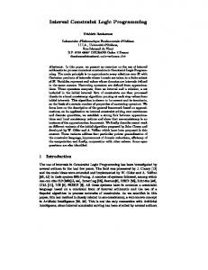
2.3. The combustion chamber problem The example problem involving the design of a combustion chamber of an internal combustion engine is based on the example developed by Wagner and Papalambros [40]. For this example, we assume a flat head design as depicted in Figure 5. The design variables are the cylinder bore (b), compression ratio (cr), exhaust valve diameter (dE), intake valve diameter (dI), and the revolutions per minute at peak power (w). The objective is to minimize the negative specific power, which is equivalent to the original objective of maximizing the brake power per unit engine displacement F. The constraints can be seen in Appendix 1.
Figure 5: Combustion Chamber [40]
8/15
Wagner and Papalambros [40] present a result of b=83.3 mm, dI=40.5 mm, dE=33.6 mm, cr=9.45, w=6.23 rpm×1000, and F=60.7 BKW/V for brake power per displacement for the 1.86L four-cylinder engine.
2.4. The OpAC and WopAC NCSP libraries The NCSP system used is OpAC and WopAC libraries (IRIN Lab of Nantes University, France) for outer and inner CP approximations [14]. The graphical visualizer of CP enumerated boxes is the USV system (Universal Solution Viewer) of IRIN Lab [6]. The tool allows users to solve numerical constraint satisfaction problems (NCSPs). Given a system of nonlinear constraints over the real numbers, it computes a set of solutions through a process based on i) local consistency techniques (a cooperation of hull consistency and box consistency techniques, cf. [1]) for pruning domains and ii) bisection for branching. The solver computes either an inner or outer approximation of the real solution set. The outer approximation guarantees completeness (all solutions in the input are retained in the domains), whereas the inner approximations guarantee soundness (each approximation does not retain any non-solutions).
2.5. The experimental protocol The Combustion Chamber is a processor from 5 DVs (B, Di, De, Cr, W) into one PV, variable F, that the designer would like to maximize. As presented in Figure 1, there are two types of relations: Engineering Constraints linking input variables (B, Di, De, Cr, W) and Performance Constraints giving output F. These constraints are given in Appendix 1. Our detailed protocol (see Figure 6) consists in: 1) Starting from initial variable domains {B = [70.0, 90.0]; Di = [25.0, 50.0]; De = [25.0, 50.0]; Cr = [6.0, 12.0]; W = [5.25, 12.0]; F = [30.0, 80.0]}, we enumerated all the a priori feasible sixdimensional boxes {B,Di,De,Cr,W,F} of 0.1 approximate size. This results in 3958 boxes (named Design Space #1) that we collected in the USV graphic visualizer. The USV system provided us with the minimal and maximal bounds of these variables: {B = [79.2188, 83.3333]; Di = [35.217, 36.9902]; De = [29.2388, 31.7864]; Cr = [8.47842, 9.30116]; W = [5.25, 6.38391]; F = [53.966, 59.8016]}. It can be noticed that the optimal solution of 60.7 provided by Wagner and Papalambros [40] did not comply with all the constraints. 2) We chose the Central Composite Design from the three types of DOEs {Central Composite Design, Latin Hypercube Design, Uniform Design}. 3) We adopted the reduced domains {B = [79.0, 83.4]; Di = [35.0, 37.0]; De = [29.0, 32.0]; Cr = [8.45, 9.35]; W = [5.25, 6.4]}, which are slightly larger than the min-max bounds previously found, for the DOE generation. 4) We limited our study to a Response Surface metamodel type of linear and quadratic polynomial approximations. 5) We replaced the initial Performance Constraint by the fitted MM (see Appendix 1). Starting from the same domains used for the DOE generation and with {F = [53.5, 62.5]}, we enumerated all the a priori feasible six-dimensional boxes of 0.1 side. We collected these boxes in USV to represent Design Space #2. 6) We compared both design spaces. The two enumerations were made with the OpAC outer approximation library only.
9/15
2) Choice of a DOE type 1) Narrowed domains of input variables
B Di De Cr W
Engineering Constraints linking input variables
Performance Constraints giving output F
F
Design Space #1
3) Design of Experiments (DOE)
B Di De Cr W
Engineering Constraints linking input variables
4) Choice of an MM type
5)Metamodel (MM) giving output F
F
Design Space #2
6) Comparizon of Design Spaces Figure 6: Our detailed protocol
2.6. Searching for a compromise between metamodel fidelity and CP precision Our objective was to find an overall good strategy for resulting in a precise design space. But, we know that: -
The higher the order of Response Surface Metamodel and the less polynomial terms are neglected, then the better the metamodel fidelity is. Such a fidelity has a price: an important number of additive monomial terms.
-
The shorter a function and the less the numbers of the same variable occurrences, the more precise the reduction/narrowing/tightening of the function domain.
A compromise clearly appears. The general form of a second-order RSM metamodel with five input variables (B, Di, De, Cr, W) is given by the formula: 2
2
2
F = a 0 + a1 B + a 2 Di + a3 De + a 4 C r + a5W + a 6 B 2 + a7 Di + a8 De + a9 C r + a10W 2 + a11 B Di + a12 B De + a13 B C r + a14 B W + a15 Di De + a16 Di C r + a17 Di W + a18 De C r + a19 De W + a 20 C rW Instead of choosing this regression formula with 20 terms, we looked for neglecting the terms with few influence on F. It led us to a regression on 17 terms while ignoring the coupling terms {Di De , De C r , De W } : F = −113.3539 + 0.7313 B + 2.8146 Di − 0.3111 De + 1.5154 Cr + 7.5478W 2
2
2
− 0.008 B 2 − 0.0731 Di + 0.0039 De − 0.1443Cr − 4.1265W 2 − 0.0001 B Di + 0.0009 B De − 0.0002 B Cr + 0.1778 BW + 0.0682 Di Cr + 0.6493 Di W + 0.1520 Cr W
We term the 2nd order metamodel (for a 27pt Central Composite Design) under this form: MM2 order-raw. nd
Granvilliers et al recall in [15] that the function form is of first importance for the domain precision of the function. Indeed: -
The dependency problem of interval arithmetic is characterized by the fact that “a variable is replaced with its domain during interval evaluation; as a consequence its occurrences are
10/15
decorrelated” resulting in a greater function domain. Thus, one has to exert to make disappear multiple occurrences of the same variable as much as possible. -
As a consequence, the subdistributivity law, characterized by the fact that the domain of x × ( y + z ) is included or equal to the domain of x × y + x × z , encourages to factorize expressions. Horner forms, Bernstein forms and nested forms are different way to factorize a function [15].
In our case, the first-order term of a variable and its square term can be collapsed into an expression with a unique occurrence of the variable, following the formula:
a x + b x2 = −
a2 a +bx+ 4b 2b
2
One can immediately check on an example that such transformation results in tighter domains. Considering the following expression equality: 4 x − x 2 = 4 − ( x − 2 )2 , one can notice that the expression with only one occurrence is more efficient in the narrowing operation:
4 x − x 2 ∈ [− 1,4] x ∈ [0,1] ⇒ 4 − ( x − 2 )2 ∈ [0,3] For the remaining second-order terms of our RSM metamodel, we chose to put them in a cross nested form (see Ceberio et al [5]). The factorization is then performed in priority with the variable of greater number of occurrences, here variable B. Finally, the raw form of our second-order metamodel becomes: 2 2 2 2 2 a a a a a F = a0 − 1 − 2 − 3 − 4 − 5 4a 6 4a 7 4a8 4a 9 4a10 2
2
2
a a a a + a 6 B + 1 + a 7 Di + 2 + a8 De + 3 + a 9 C r + 4 2a 6 2a 7 2a 8 2a 9 + B(a11 Di + a12 De + a13 C r + a14W ) + Di (a16 C r + a17W ) + a 20 C r W
2
a + a10 W + 5 2a10
2
Note that the dependency problem is also partially (locally, see [15]) overcome by the use of the box consistency narrowing technique. We term the 2nd order metamodel under this form: MM-2ndorderformed. F = −68.3226 − 0.008 (B − 45.7062) − 0.0731 (Di − 19.2517) + 0.0039 (De − 39.8846) − 0.1443 (Cr − 5.2508) − 4.1265 (W − 0.91455) 2
2
2
2
+ B (− 0.0001 Di + 0.0009 De − 0.0002 Cr + 0.1778W ) + Di (0.0682 Cr + 0.6493W ) + 0.1520 Cr W
Lastly, the first-order metamodel (for a 27pt Central Composite Design) is termed: MM-1storder and is given by: F = −70.2341 + 0.4905 B + 1.9365 Di − 1.363W
11/15
2
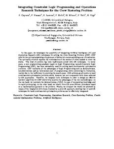
2.7. Results and comments
Figure 7: 3D projection of the design space on (Di,De,F): Design Space #1 at left and Design Space #2 with respectively MM-2ndorder-raw and MM-2ndorder-formed metamodels. We obtained the design spaces (see figure 7) but we were embarrassed to compare them. The first reflex would be to operate subtractions and intersection between design spaces so as to get quantitative measures of proximity: -
DS#1 – DS#2 represent the missed design space.
-
DS#2 – DS#1 represent the invalid design space.
-
DS#1 ∩ DS#2 represent the common design space.
Three measures of comparison could be the volume of these spaces as a percent of DS#1 volume. But these space subtraction and intersection are not trivial when elementary boxes are not cut at the same locations. Fortunately, the calculation of the three volumes can be approximated by Monte Carlo generation of design points followed by a determination of their set properties. This is sometimes referred to as Monte Carlo integration. This utility is under development.
3. Conclusion We presented the benefits that a “set-based design”, to oppose to a current “point-to-point” or tryand-test design, could have in an industrial design project in terms of time-to-market lowering and design quality improvement. Nevertheless, we mentioned that, despite the recent improvements in Constraint Programming techniques over continuous domains, NCSP environments should integrate a richer designer semantic with more usable implementation tools so as to tackle industrial problems of practical size and interest. The problem of taking mechanical performances assessed through lengthy simulations into account is one of the most preoccupying impediment. We proposed a framework to compile at best a hard engineering performance assessment into a tractable approximated but analytical constraint that engineers could take into account with their other constraints. Metamodeling approaches were chosen because of the collection of techniques and existing strategies to fit to a particular issue. Here a compromise clearly appears between the metamodel fidelity and the resulting precision in an NCSP environment. We proposed an engineering case-study in the place of the combustion chamber problem [40]. As soon as quantitative measures of design space proximity will be available, we will try to determine some heuristics for an acceptable MM/NCSP compromise: which design of experiments (DOE), which MM (metamodel) type, which MM order, how many terms for analytical constraints, and which analytical form? Other studies like the influence of the MM intrinsic fidelity on the measures of design space proximity would also be interesting.
12/15
4. References [1] Benhamou F., Goualard F., Granvilliers L., Puget J.-F., (1999), Revising Hull and Box Consistency, in Procs. of ICLP'99, The MIT Press: Las Cruces, USA, vol. [2] Benhamou F., Mc Allester D., Van Hentenryck P., (1994), Clp(intervals) revisited. in Logic Programming. [3] Bourne A., Clément A., Foussier A., Saulais J., Sicard M., (1990), JADE : un jeu d'outils d'aide à la décision technologique, in Outils et applications de l'intelligence artificielle en CFAO, Yvon Gardan, Hermès, vol., p. 148-161. [4] Box G.E.P., Draper N.R., (1987), Empirical Model Building and Response Surfaces, New York, John Wiley & Sons. [5] Ceberio M., Granvilliers L., (2000), Solving Nonlinear Systems by Constraint Inversion and Interval Arithmetic. in Proceedings of AISC'2000, 5th International Conference on Artificial Intelligence and Symbolic Computation, Madrid, Spain, 127-141. [6] Christie M., (2002), USV: user manual, IRIN Lab, Nantes University: Nantes, France. [7] Degirmenciyan I., Foussier A., Chollet P., (1994), Un conciliateur/coordinateur pour une conception simultanée. Revue de CFAO et d'informatique graphique, vol.: p. 889-911. [8] Draper N.R., Lin D.K.J., (1990), Connections Between Two-Level Designs of Resolutions III and V. Technometrics, vol. 32(3): p. 283-288. [9] Faltings B., Djamila H., Smith I., (1992), Dynamic Constraint Propagation with Continuous Variables. in ECAI-92, 754-758. [10] Fang K.-T., Lin D.K.J., Winker P., Zhang Y., (2000), Uniform Design: Theory and Application. Technometrics, vol. (42): p. 237-248. [11] Finch W.W., (1999), Set-based models of product platform design and manufacturing processes. in DETC'99: ASME 1999 Design Engineering Technical Conference, Las Vegas, USA, Paper number DETC99/DTM-8763. [12] Finch W.W., Ward A.C., (1997), A set-based system for eliminating infeasible designs in engineering problems dominated by uncertainty. in DETC'97: ASME / Design Engineering Technical Conference, Sacramento, California, DETC97/DTM-3886. [13] Fischer X., (2000), Stratégie de conduite de calcul pour l'aide à la decision en conception mécanique intégrée - Application aux appareils à pression. Thèse de l'ENSAM, [14] Goualard F., Christie M., (1999), C++ OpAC and WOpAC libraries for outer and inner Constraint Programming approximations, IRIN Lab, Nantes University: Nantes, France. [15] Granvilliers L., Benhamou F., Huens E., (2001), Constraint Propagation (chapter 5), in COCONUT Deliverable D1 Algorithms for Solving Nonlinear Constrained and Optimization Problems: The State of the Art, The Conconut Project, vol., p. 113149. [16] Gu L., (2001), A Comparison of Polynomial Based Regression Models in Vehicle Safety Analysis. in ASME Design Engineering Technical Conferences - Design Automation Conference (DAC), September 9-12, 2001, Pittsburgh, PA, Paper No. DETC2001/DAC21063. [17] Hyvönen E., (1989), Constraint reasoning based on interval arithmetic. in IJCAI-89, 1193-1198. [18] Hyvönen E., (1992), Constraint reasoning based on interval arithmetic: the tolerance propagation approach. Artificial Intelligence, vol. 58: p. 71-112. [19] Janssen P., (1990), Aide à la conception : une approche basée sur la satisfaction de contraintes. Thèse de doctorat, Université de Montpellier des Sciences et Techniques du Languedoc. [20] Kleijnen J.P.C., (1975), A Comment on Blanning's Metamodel for Sensitivity Analysis: The Regression Metamodel in Simulation. Interfaces, vol. 5: p. 21-23. [21] Lhomme O., (1993), Consistency techniques for numeric CSPs. in IJCAI-93, Chambéry, France, 232-238. [22] Lhomme O., Gotlieb A., Rueher M., Taillibert P., (1996), Boosting the interval narrowing algorithm. in ICLP: MIT Press. [23] Lottaz C., Clément D.E., Faltings B.V., Smith I.F.C., (1999), Constraint-Based Support for Collaboration in Design and Construction. Journal of Computing in Civil Engineering, vol. 13(1): p. 23-35. [24] Lottaz C., Sam-Haroud D., Faltings B.V., Smith I., (1998), Constraint Techniques for Collaborative Design. in IEEE International Conference on Tools with Artificial Intelligence. [25] Lottaz C., Smith I.F.C., Robert-Nicoud Y., Faltings B.V., (2000), Constraint-based support for negotiation in collaborative design. Artificial Intelligence in Engineering, vol. 14: p. 261-280. [26] Lottaz C., Stouffs R., Smith I., (2000), Increasing Understanding during Collaboration Through Advanced Representations. ITcon, vol. 5. [27] McAllister C.D., Simpson T.W., (2001), Multidisciplinary Robust Design Optimization of an Internal Combustion Engine. in ASME Design Engineering Technical Conferences, Pittsburgh, USA/PA, sept 9-12, 2001, Paper number DETC2001-DAC-21124.
13/15
[28] McKay M.D., Beckman R.J., Conover W.J., (1979), A Comparison of Three Methods for Selecting Values of Input Variables in the Analysis of Output from a Computer Code. Technometrics, vol. 21(2): p. 239-245. [29] Meckesheimer M., Barton R.R., Simpson T.W., Limayem F., Yannou B., (2001), Metamodeling of Combined Discrete/Continuous Responses. AIAA Journal (American Institute of Aeronautics and Astronautics), vol. 39(10 (october 2001)): p. 1950-1959. [30] Merlet J.-P., (2001), Projet COPRIN : Contraintes, OPtimisation, Résolution par INtervalles, Rapport, INRIA SophiaAntipolis, 21 septembre 2001. [31] Myers R.H., Montgomery D.C., (1995), Response Surface Methodology: Process and Product Optimization Using Designed Experiments, New York, John Wiley & Sons. [32] Otto K., Antonsson E., (1993), The Method of Imprecision Compared to Utility Theory for Design Selection Problems. in ASME/DTM '93: Design Theory and Methodology, 167--173. [33] Otto K., Antonsson E., (1993), Propagating Imprecise Engineering Design Constraints. in IEEE International Conference on Fuzzy Systems, Yokohama, Japan, 375-382. [34] Rueher M., Solnon C., (1997), Concurrent Cooperating Solvers over Reals. Reliable Computing, vol. 3(3): p. 325-333. [35] Sam J., (1995), Constraint Consistency Techniques for Continuous Domains. Ph.D. Thesis number 1423, Ecole Polytechnique Fédérale de Lausanne, EPFL. [36] Shen W., Barthes J.-P., El Dashan K., (1994), Propagation de contraintes dans les systèmes de CAO en mécanique. Revue Internationale de CFAO et d'infographie, vol. 9(1-2): p. 25-40. [37] Simpson T.W., Peplinski, J.D., Koch P.N. and Allen, J.K., (2001), Metamodels for Computer-based Engineering Design: Survey and recommendations. Engineering with Computers, vol. 17: p. 129-150. [38] Van Hentenryck P., Michel L., Benhamou F., (1998), Newton: Constraint Programming over Nonlinear Constraints. Science of Computer Programming, vol. 30(1-2): p. 83-118. [39] Vargas C., (1995), Modélisation du processus de conception en ingénierie des systèmes mécaniques. Mise en oeuvre basée sur le propagation de contraintes. Application à la conception d'une culasse automobile. Ecole Normale Supérieure de Cachan. [40] Wagner T.C., Papalambros P.Y., (1991), Optimal Engine Design Using Nonlinear Programming and the Engine System Assessment Model, Technical Report, Ford Motor Co. Scientific Resaerch Laboratories, Dearborn Michigan and the Department of Mechanical Engineering at the University of Michigan, Ann Arbor, August 15 1991. [41] Ward A.C., Liker J.K., Sobek D.K., Cristiano J.J., (1994), Set-based concurrent engineering and Toyota. in DETC'94: ASME / Design Engineering Technical Conference, Sacramento, California, DETC94/DTM, 79-90. [42] Wood W.H., (2001), A view of design theory and methodology from the standpoint of design freedom. in ASME Design Engineering Technical Conferences, Pittsburgh, USA/PA, sept 9-12, 2001, Paper number DETC2001-DTM-21717. [43] Yannou B., (1998), Chapitre 19 : Les apports de la programmation par contraintes en conception, in Conception de produits mécaniques : méthodes, modèles et outils, Tollenaere M. Editor, Hermes, vol. ISBN 2-86601-694-7, p. 457-486.
14/15
set set set set set set
variable variable variable variable variable variable
B = [79.0, 83.4]; Di = [35.0, 37.0]; De = [29.0, 32.0]; Cr = [8.45, 9.35]; W = [5.25, 6.4]; F = [53.5, 62.5];
set const Pi = 3.1415927; set const G = 1.33; set const K_1 = 1.2; set const K_2 = 2.0; set const K_3 = 0.82; set const K_4 = 0.83; set const K_5 = 0.89; set const K_6 = 0.6; set const K_7 = 6.5; set const K_8 = 230.5; set const K_9 = 2.3e6; set const K_10 = 1.6e6; set const K_11 = 1.0/64.0; set const K_12 = 0.125; set const L_1 = 400.0; set const L_2 = 200.0; set const V = 1.859e6; set const Cs = 0.44; set const Nc = 4.0; set const Q = 43958.0; set const Pincv = Pi*Nc/V; set const Pincvcs = Pincv*Cs; set const P_1 = L_1/(K_1*Nc); set const P_2_square = 4.0*K_2/(Pincv*L_2); set const P_3 = 9.428e5*4.0/(Pincvcs*K_6); set const P_4 = 3.6e6/(K_8*Q);
DECLARATIONS
Constants and variables
constraint constraint constraint constraint constraint constraint constraint constraint constraint constraint constraint
c1(B); c2(B); c3(Di, De, B); c4(Di, De); c5(Di, De); c6(W, Di); c7(Cr, B); c8(W); c9(Nutad, Sv); c10(B, S); c11(B, S);
CONSTRAINTS
set set set set set set set set set set set
15/15
c1(B) = B-P_1 < 0; c2(B) = sqrt(P_2_square)-B < 0; c3(Di, De, B) = Di+De-K_3*B < 0; c4(Di, De) = K_4*Di-De < 0; c5(Di, De) = De-K_5*Di < 0; c6(W, Di) = P_3*W-pow(Di,2) < 0; c7(Cr, B) = Cr-13.2+0.045*B < 0; c8(W) = W-K_7 < 0; c9(Nutad, Sv) = P_4-Nutad+Sv < 0; c10(B, S) = B - 0.7*S > 0; c11(B, S) = B - 1.3*S < 0;
set function S = 4.0/(Pincv*pow(B,2)); set function Sv = 0.83*((8+4*Cr)+1.5*(Cr1)*4.0*B/S)/((2.0+Cr)*B); set function Nutad = 0.8595*(1-exp((1-G)*log(Cr)));
Engineering constraints linking input variables (B,Di,De,Cr,W) DECLARATIONS
5.1. Appendix 1: The Combustion Chamber problem
5. Appendices
DECLARATIONS set constraint c13(F,B,Di,De,Cr,W) = -113.3539 + 0.7313*B + 2.8146*Di –0.3111*De + 1.5154*Cr + 7.5478*W–0.008* pow(B,2) – 0.0731* pow(Di,2) + 0.0039* pow(De,2) – 0.1443* pow(Cr,2) – 4.1265*pow(W,2) – 0.001*B*Di + 0.0009*B*De – 0.0002*B*Cr + 0.1778*B*W + 0.0682*Di*Cr + 0.6493*Di*W + 0.1520*Cr*W – F == 0; CONSTRAINTS c13(F,B,Di,De,Cr,W);
MM-2 order-raw Metamodel system (Secondorder response surfaces, based on 27pt Central Composite Design, in a raw form)
nd
CONSTRAINTS c12(F, W, BMEP);
DECLARATIONS set const K_0 = 1/120; set const Af = 14.6; set const Rho = 1.225; set const P_0 = Rho*Q/Af; set function Vp = 2.0*W*S; set function Nut = Nutad-0.083*Sv*sqrt(1.5/W); set function Nuvb = 1.067-(0.038*exp(W-5.25)); set function Nuv = Nuvb*(1.0+5.96e3*pow(W,2))/(1.0+pow(9.428e5*4.0*W/(Pincvcs*pow(Di,2)),2)); set function FMEP = 4.826*(Cr9.2)+(7.97+0.253*Vp+9.7e-6*pow(Vp,2)); set function IMEP = Nut*Nuv*P_0; set function BMEP = IMEP-FMEP; set constraint c12(F, W, BMEP) = F- K_0*W*BMEP == 0;
Initial Combustion Chamber system
Specific parts of declarations and Performance Constraints giving output F