In GIS, we can classify buffer primitives as point buffering operations, line
buffering operations, and ... Consider the example given in figure 3. Here we can
see ... in a similar way. Next, we perform a line intersection test to eliminate
common.
Buffer Operations in GIS Nagapramod Mandagere, Graduate Student, University of Minnesota
[email protected] SYNONYMS GIS Buffers, Buffering Operations DEFINITION A buffer is a region of memory used to temporarily hold output or input data. In case of Geographical Information Systems, the units of buffering are points, lines, and polygons. Buffer operation refers the creation of a zone of a specified width around a point or a line or a polygon area. It is also referred to as a zone of specified distance around coverage features. There are two types of buffers: constant width buffers and variable width buffers. Both types can be generated for a set of coverage features based on each features attribute values. These zones or buffers can be used in queries to determine which entities occur either within or outside the defined buffer zone. Analogous to buffering in raster GIS is distance analysis. In practical situations, one needs to buffer multiple regions (points, lines and polygons) simultaneously. This gives rise to the idea of buffer allocation and replacement. Data movement happens by making use of primitive buffer operations such as point buffer operation, line buffer operation and polygon buffer operations. Buffer management involves the process of allocation of buffers and replacement of buffers when not needed. Several allocation policies and replacement policies that have been used in the context of memory buffers in computer science are directly applicable here. HISTORICAL BACKGROUND Spatial data usually consist of different types of objects. Object types include points, lines and polygons. The idea of providing primitives for basic buffer operations started soon after the inception of spatial databases themselves. Working on atomic units of points was soon found to be not a very scalable option. The search for a more scalable and computationally efficient technique led to the introduction of buffer primitives. SCIENTIFIC FUNDAMENTALS In GIS, we can classify buffer primitives as point buffering operations, line buffering operations, and polygon buffering operations. Buffering points: A point is the basic unit of resolution in any GIS system. Buffering point data involves the creation of a circular polygon about the point of interest. The radius of this circular polygon is called the buffer distance. In this scheme the buffer distance or the radius of the circle could be fixed for all points in a layer or the user could specify it. If multiple points in the same layer are being buffered, then buffer distances of each point are either specified in an attribute table or a look up table. If one is buffering multiple
points in the same layer, then the buffering algorithms check for overlaps in each point’s buffer and remove the overlapping sections.
Figure 1. Buffering Multiple Points If multiple point buffers intersect or overlap, as illustrated in Figure 1, then the system takes all the overlapping polygons and combines then into one or more polygons that represent a layer. This process of removal of overlapping sections involves the use of intersection and dissolves. In Figure 2, polygons A, B, and C describe the layer with all the eight points of interest.
Figure 2. Removal of Overlaps The point to note here is that now one needs to also keep track as to whether a polygon lies within the buffer zone or outside a buffer zone. For this purpose, the system maintains a table of constituent polygons and their corresponding attribute (inside or outside) per layer. The table below shows the mapping for the layer considered in Figure 2. Polygonal Region A B C
Inside 1 0 0
Buffering Lines: Buffering lines is a little more complicated than buffering point data. This is mainly due to the fact that lines can be made up of multiple segments. Line segments are handled independently of each other. Consider the example given in figure 3. Here we can see two line segments. First, let us consider L1 with end points (A1,B1) and (A2,B2).
Using these coordinates one can calculate dx and dy between the two end points. Now, we can represent two parallel lines at a distance of m (buffer distance) from L1 using the sine and cosine components of line L1 along with m, the buffer distance.
Figure 3. Line Buffering After determining the two parallel line segments, we process any remaining line segments in a similar way. Next, we perform a line intersection test to eliminate common regions or overlapping regions. Finally, we add the bounds to the parallel buffers by capping the start point and end point of the line with half circular polygons of radius m or bounding rectangles.
Figure 4. Multiple Intersecting Line Segments The task of looking for overlaps between line buffers works as follows. If we have multiple lines being buffered, each composed of multiple line segments as shown in figure 4. Again, the same process used for point buffers is applied. As a result we get one or more polygons representing a layer. Figure 5 illustrates the same along with the concept of polygon table. Here polygon A is inside the buffer zone and polygon B is outside of the buffer zone.
Figure 5. Line Buffering with Overlap Removed
Buffering Polygons:
Buffering of polygonal surfaces uses most of the same concepts used for line buffering. The only significant change is that the polygon buffer is created on only one side of the line that defines the polygon. In polygon buffering two options are available, namely – an outside polygon which surrounds/contains the polygonal surface under consideration or an inside polygon that is contained inside the polygonal surface under consideration. Figure 6 illustrates the concept of polygonal buffering.
Figure 6. Polygon Buffering
Accuracy of Buffer Operations: The accuracy of buffer operations depends completely on the quality of the spatial data available. The quality of the spatial data is limited by the accuracy of the sources such as maps and satellite images. Data acquisition and manipulation techniques such as map digitization, photo interpretation, and map transformation often introduce errors in the data [4][5]. This phenomenon is often referred to as error propagation. The accuracy of positional information can have a profound impact on buffer operations. To illustrate, consider the following example of point buffering. In figure 7, O is the actual or original data point and X is the observed data point. The process of data acquisition and manipulation has caused the observed point to be e units away from its original position.
Figure 7. Errors in Point Buffering Now, when point buffering algorithms are applied to the observed point X with a buffer distance of r units, we get a circular buffer region. But, if we were to apply the same buffering algorithm to point O, we would end up with a different buffer region. As is evident from the figure, certain portions which should have been in the resultant buffer region are no longer part of the resultant buffer region and some portions which were not intended, have been included in the resultant buffer region. These types of errors are usually referred to as errors of omission and errors of commission, respectively. A
detailed analysis of the effect of positional accuracy on errors of commission and omission can be found in [3]. Line buffering algorithms also suffer a similar problem due to inaccuracy of positional data. Consider Figure 8,
Figure 8. Errors in Line Buffering Here, (A1,B1) and (A2,B2) are the original points that form the line segment. Due to positional errors points, (A2,B2) appear to be at (E1,E2). Figure 8 shows the effect of applying line buffering operations described earlier to the two line segments. The resulting buffer regions and the errors of commission and omission are shown in Figure 8. For a detailed analysis of the relationship between positional accuracy and errors of commission and omission, the reader may refer to [3]. The algorithms used for various buffer operations have some impact on the extent of errors of omission and commission. But the buffer depth chosen for these algorithms can have a profound impact on the errors of commission and omission. Hence one has to exercise some caution when selecting the buffer depths in algorithms which employ user defined buffer depths. KEY APPLICATIONS In this section, first we consider real world examples where buffering of points, lines or polygons are used. Next, we explore various schemes which make use of buffer operations. Consider the following scenario for point buffering. The University of Minnesota wants to make sure that every inch of the main campus is covered by a wireless network. The university has deployed a large number of wireless access points at various points on campus. Now, the goal is to find if the wireless network covers all points in the map shown. For the buffer distance, let’s assume that the wireless range of each access point is 500m. Now, lets apply the concept of point buffering for the wireless access points with a buffer distance of 500m. The next step is to remove overlaps. Now the region that do not fall under the resultant buffer polygon(s) are the regions that do not have any wireless network coverage. Next, let us look at a real world application of line buffering. Consider a huge ship, the boundary of which can be modeled as a set of line segments. The owners of the ship want to know if all the deck areas near the edges have been water proofed. For this example, let us say that only deck areas within a distance of 50 feet from any edge need to be water proofed. Now, by applying line buffering to all line segments that form the exterior of the ship with a buffer distance of 50 feet, we obtain a polygonal area that
needs to be water proofed. By checking if all area under this polygon have been water proofed, the owner achieves his/her goal. Now, let us look at a real world application of polygonal buffering. Consider a scenario where the university is hosting a special event and hence is planning to create a few make-shift parking spots around the campus. Now, a few rules need to be followed, i.e., no vehicle can be parked with in 50 feet of any campus building and all parking spots need to be off road parking. We can model this situation by buffering polygons around each campus building with a buffer distance of 50 feet. Here we make use of outer polygonal buffering. After eliminating the overlaps, all areas that do not fall under the resultant buffer polygon(s) are free for parking. Buffer Allocation: Buffer or memory is often a limited shared resource. Often a need arises to buffer multiple regions such as points, lines or polygons simultaneously. Multiple applications or streams share common buffers. Buffer allocation involves the process of segmenting or dividing these buffer regions amongst competing applications or processes. Different allocation schemes have been proposed in computer science. Most of them can be readily applied to GIS with minimal modifications. One could perform static allocation or dynamic on demand allocation of buffers. Dynamic allocation is more complex to implement but more resilient to changes. Buffer regions could be strictly partitioned between competing processes or a global buffering scheme could be used. Pre-fetching of Buffers: In certain situations one could predict buffer access patterns. For instance, if a GIS application is working over a specific region of a map, one could think of buffering all polygons that are adjacent to the polygon under consideration. This works like a look ahead of a pre-fetch mechanism. This pre-fetching can often lead to huge performance improvement in terms of response times for queries. Another mechanism of pre-fetching uses the application domain knowledge to pre-fetch relevant regions. Specifically, an application can predict its own access pattern and inform the system to pre-fetch certain regions. Again, different pre-fetching schemes are used, depending on the application domain. Buffer Replacement: A buffer is a limited region of memory. Since the data set size is larger than the buffer size, the need arises to replace existing data in order to accommodate new data. This process is referred to as buffer replacement. A number of buffer replacement algorithms that have been proposed in computer science are directly applicable here. Some of the most popular algorithms include, Not Recently Used (NRU), Least Recently Used (LRU), Clock Algorithm, Second Chance, Working Set, First In First Out (FIFO), Last In First Out (LIFO) and Aging. Out of these, LRU and its variants are the most popular algorithms. In GIS applications, FIFO might make more sense if there is little repeatability of buffer regions. The choice of buffer replacement algorithm completely depends on the application for which it is being used.
FUTURE DIRECTIONS Buffer operations have been around for a while now. Most work now focuses on intelligent use of buffer operations. One of the interesting fields of research is predictive and adaptive buffering techniques. Since any improvement in these techniques can have a drastic impact on spatial query response times, much effort is ongoing in this field. RECOMMENDED READING [1] Tutorials on Topics in GIS: http://www.sli.unimelb.edu.au/gisweb/BuffersModule/BuffSelect.htm [2] Glossary and definition of key terms in GIS: http://en.mimi.hu/gis/buffer.html [3] Yukio Sadahiro, Buffer Operations on Spatial Data with limited Accuracy, In Transactions in GIS, 2005, 9(3): pages 323-344 [4] Heuvelink G B N, Propagation of Errors in Spatial Modeling with GIS, International Journal on Geographical Information Systems 3: Pages 303-322 [5] Maffini G, Arno M, Bitterlich W, Observation and Comments on generation and treatment of errors in digital GIS data, In Goodchild M F and Gopal S , The Accuracy of Spatial Databases. London, Taylor and Francis: Pages 55-67