Jul 7, 2010 - sponding to points on the surface of the scanned object. ... ity intensity and curvature to divide the point cloud into feature regions .... border. (center) The feature boundary region. .... region we also obtain the principal axes.
Noname manuscript No. TR-CS-2010-04, July 7, 2010
Building Editable B-rep Models from Unorganized Point Clouds V. Stamati and I. Fudos
Technical Report: Computer Science Department TR-2010-04
Abstract We present a novel integrated approach to reverse engineering point clouds by producing fully editable feature-based Boundary Representation (B-rep) models. We use point cloud morphology analysis techniques to extract features from a 3D point cloud. We then reconstruct the boundary contours of features using a fast and efficient fitting approach employing a sequence of piecewise rational Bezier curves that are G1 continuous. We introduce a technique for reconstructing the features derived from the point cloud using solid modeling techniques, such as sweeping, skinning and covering, providing editability and model re-design capability. The solid modeling techniques selected for feature reconstruction depend on the morphology of the point set and the complexity of the reconstructed contours of the feature. We support parameter definition on each feature to render attributes such as construction techniques, adjacency and other topological characteristics. A feature connectivity graph is derived and used for producing a feature assembly plan that describes the reconstruction process of the Brep model. Inter- and intra- feature constraints are imposed to ensure that the final reconstructed model is editable, robust and accurate. We offer examples of using our reengineering system to demonstrate the feasibility of this method and its unique editing capabilities.
1 Introduction Reverse engineering is a general concept that can refer to various fields, such as software technology, product design and manufacturing or archaeological site reconstruction [9]. In solid modeling and Computer-Aided Design, reverse engineering aims to analyze a real object and determine its characteristics and structure mechanisms, with V. Stamati and I. Fudos Department of Computer Science, University of Ioannina, GR45110, Ioannina, Greece E-mail: {vicky,fudos}@cs.uoi.gr
focus on editability and manufacturability. The data concerning the physical object are obtained by various methods. Common methods include 3D laser scanning or photogrammetry methods that produce a point cloud corresponding to points on the surface of the scanned object. In the context of solid modeling and CAD, reverse engineering is the process of obtaining a B-rep model from measurements acquired by scanning an existing physical model [23]. Reverse engineering is vital for industry because the computer models acquired help improve the quality and efficiency of designs and also speed up the analysis and manufacturing process. The aim of this work is to introduce an integrated method for reverse engineering objects of mechanical or freeform design to obtain fully editable feature-based Brep models that can be reproduced or modified before production. More specifically, our approach partitions a 3D point cloud into components corresponding to features, so as to create an editable and parameterized solid model described by its various interconnected features. This type of model provides the user-designer with the capability of editing, redesigning and reproducing the original object, according to his preferences and needs, by editing the features of the model [8]. The information flow in our system is summarized in Figure 1. We begin from a 3D point cloud which we have preprocessed to remove duplicate points and an STL (stereolithography) file of the point cloud. An STL file is a file describing the model as a triangular mesh. This file format provides the vertices of each triangle of the mesh and the corresponding normal vectors. We perform segmentation of the point cloud into subsets by detecting features using a point-wise characteristic called point concavity intensity and the local surface normal vector variations that measure mesh curvature. We apply a region growing method based on variations of point concavity intensity and curvature to divide the point cloud into feature regions and regions corresponding to their boundaries. The boundary regions are approximated with cubic rational Bezier curves through a fast and efficient curve
2
ture components so that they can be used seamlessly in complex solid modeling operations.
2.1 Feature Definition
Fig. 1 Feature-based Reverse Engineering Platform Data Flow
approximation method that we have developed. The resulting contours are used in combination with the feature regions to reconstruct each feature using solid modeling operations. The resulting features are then combined using a feature assembly plan based on a feature adjacency graph to construct the final B-rep model. Parameters and constraints are defined on the feature components to provide for editability and robustness. This paper makes the following technical contributions: – Describes a methodology for reconstructing the features of the object using solid modeling techniques. – Presents a feature assembly plan based on a connectivity graph of the model’s feature elements. – Introduces parameters and constraints to allow for editability. – We report on the development of a prototype system called Re-FACE (Re-Engineering with Feature Assembly plans using Constraints for advanced Editability) and present some reconstruction examples. Section 2 presents an overview of our approach to detecting and extracting features from a 3D point cloud based on point concavity intensity and surface normal variation. A fast and efficient curve approximation method for fitting cubic rational Bezier curves to 3D points is also presented in Section 2. Section 3 focuses on reconstructing features using solid modeling operations. Section 4 focuses on using a connectivity graph for building a construction plan to create a B-rep model. In Section 5 we present reconstruction examples that verify our re-design paradigm. Section 6 offers a brief comparison to other reengineering approaches. Section 7 provides conclusions.
2 Feature Formation Our Brep model reconstruction method is based on reengineering objects by exploiting their morphological feature elements. In this section we outline our method used for detecting and extracting features from point clouds for the purposes of reengineering. The objects that can be reengineered by the proposed approach can be either of mechanical or freeform design. It is also important for feature construction and assembly to provide tools for reconstructing the boundary contours of the detected fea-
“Feature”, in computer-aided design, is a term used to describe an entire class of concepts. In general, features are generic shapes or characteristics which can be associated with certain attributes and knowledge[16]. These attributes usually describe the morphology of the object, i.e. through parameters defining its size, shape and orientation, and its behavior in a CAD model, i.e. connectivity issues, constraints and tolerances[13]. The use of features in a model provides the user-designer with the ability to edit and redesign the model[8], [15]. A user-designer can even define his own feature components to use in the design phase[7]. Given this, various systems apply the concept of features in a way compatible to the scope and aim of the respective application. In reverse engineering applications, and specifically, in reconstructing mechanical parts, features are entities traditionally used in engineering designs such as slots, holes, and bosses[21]. In reverse engineering of objects of freeform design, the term ”feature” is often used in the sense of feature lines[4], meaning edges/boundaries of an object that can be detected by changes of the surface curvature of the object[3],[6].[22] uses an intermediate data structure called a feature skeleton which is a network of curves basically representing the boundaries of surface regions. In Brep models features can also be surfaces that can be grouped together based on certain characteristics or properties. In this sense, we consider a feature as a group of points that has morphological semantics, from a design point of view. We consider how feature components that consist of feature regions and boundary curves can be used to reconstruct a complete editable B-rep model of an object. We apply solid modeling techniques to combine and obtain the entire 3D model representation. Furthermore, we introduce parameters and constraints on these features to enable editing and capturing of design intent.
2.2 Feature Detection and Extraction In [18] we have presented a feature-based approach to reengineering freeform objects from point clouds obtained by 3D laser scanners. This approach is based on discovering features on the point cloud by detecting key local changes in the morphology of the point cloud. We employ region growing, detection of rapid variation of the surface normal and the concavity intensity, i.e. the distance from the convex hull. This results in a number of regions that represent object features. More specifically, morphological features in the point cloud are detected using a characteristic called the “concavity intensity” of a point which represents the smallest
3
Fig. 4 The result of our feature detection and extraction method on the screwdriver point cloud. Fig. 2 Point cloud of a cycladic idol
feature is not continuous, by specifying additional connecting points to be included in the border contour. Our region growing method returns sets of points corresponding to the feature (feature region) and sets of points corresponding to the boundaries of the features (region border). The boundaries are used for curve approximation whereas the region points are used for surface fitting. In the following we focus on constructing smooth fitting curves for the region boundaries. For more details on our feature detection and extraction approach the reader is referred to [18] and [17]. Fig. 3 Greyscale mapping of point cloud concavity intensity values and feature regions
2.3 Feature Contour Reconstruction distance of a vertex from its convex hull. This characteristic detects concave features in the cloud. Figure 2 presents the point cloud of a cycladic idol, whereas Figure 3 displays a greyscale mapping of the concavity intensity value of each point (white color corresponds to the maximum distance whereas black corresponds to points located on the convex hull). Features are also detected by rapid variations of the surface normal. These two characteristics are combined in a region growing method that results in sets of points corresponding to individual features (Figure 3). By obtaining the features of the object we can create an editable and parameterized B-rep model described by its various connected components. This type of model provides the user-designer with the capability of editing, redesigning and reproducing the original object, depending on his preferences and needs, by editing the features of the model and the inter-feature constraint. Another example of our region growing method is shown in Figure 4, where it is applied on the point cloud of a screwdriver[20]. A short post-processing step on the feature regions may be performed manually after region growing. Specifically, we can merge two regions together to form a single region or we can split a region into two smaller regions. This is accomplished interactively by specifying vertex sequences which can form a border between the two new regions. Also we can create user-defined hardwired pointwise boundary contours to limit the behavior of the region growing method, when recalculating the regions on a portion of the point cloud. Also border correction can be carried out manually in cases where the border of a
The feature extraction method described in the previous section derives sets of points corresponding to borders of feature regions and sets of points corresponding to the feature bodies. Let CR be a contour region consisting of n 3D points. We wish to build a set of curves that best approximates this data set and captures the overall morphology of the border. We require that the method used for fitting is of low computational complexity and of low degree to avoid multiple curvature reversing. Approaches in the literature did not meet these requirements either because of slow convergence, or usage of curves of higher degree or no consideration of the fairness of the curve ([14], [24], [25]). We use an approach that fits 3D cubic rational Bezier curves to boundary point sets of features that ensures that the curve segments obtained conform to the conditions required for G1 continuity. We use an equivalent instance of the general NURB, namely piecewise rational cubic Bezier curves because the constraints we apply decrease the degrees of freedom of our problem and our requirements are well met with this low degree simpler representation, resulting in a fast converging optimization algorithm. Using piecewise rational Bezier curves we basically follow an optimization approach which can inherently rule out noisy data without affecting the shape of the boundary as a whole. Rational curves are flexible curves that can approximate complex geometry more accurately than pure polynomials of similar degrees. In general they are not preferred for reverse engineering applications in the sense that their nonlinear multivariate format is not computationally practical. However they
4
Fig. 5 Inner control point coordinates expressed in reference to the end control points
are not as expensive and time consuming when used to approximate low degree patterns. Before applying our curve approximation method on the feature borders, we perform thinning on the border region. The sequence of points representing the feature border is divided into subsets of points and curve approximation is carried out on each point subset. Curve approximation is performed with a least squares optimization procedure. Suppose Q = Q1 , Q2 , . . . , Qm is a set of ordered border points and C is an approximating rational Bezier curve given by the equation: n �
C(ui ) =
wj Pj Bj (ui ))
j=1 n �
(1) wj Bj (ui )
j=1
where n=4 for a cubic rational Bezier curve, ui is the parameter value associated with border point Qi , Pj are the control points, wj is the weight of each control point and Bj is the corresponding Bernstein polynomial. Assuming that all points of Q should be approximated by the curve, we would like to minimize the error: ei = Qi − C(ui )
(2)
The least squares problem is then to minimize the error: E=
m � i=1
ei 2 −→ E =
m �
((Qi − C(ui )))2
(3)
i=1
We partially differentiate this target function with respect to two independent variables. This results in two different systems of linear equations. To ensure G1 continuity between the Bezier curves produced by our fitting approach, we import constraints into the resulting equations. We make sure the starting point of one curve coincides with the end point of the previous curve and that the inner control points are located accordingly on the tangents of the end points (Figure 5). The solutions of the systems of linear equations are used iteratively in a two-step optimization procedure that ultimately determines the values of the weight variables and the inner control point coordinates. This is a fast curve approximation approach that produces smooth continuous curves that interpolate or pass close by the original data points. A good approximation is reached within a few iterations. In some cases, the minimal error is obtained after a single iteration.
Fig. 6 (left) A feature extracted from the point cloud and its border. (center) The feature boundary region. (right) The reconstructed boundary contour
An example of feature boundary reconstruction by means of our method is shown in figure 6. For more details on our boundary contour reconstruction approach please refer to [19],[17].
3 Feature reconstruction using solid modeling techniques Features, as used from our perspective, can be reconstructed from their regions either by surface fitting or solid modeling operations. Surface fitting constructs a surface model that conforms to the initial object from both a morphological and an aesthetic point of view, however its editing capabilities are limited to interactive pointwise modifications. Therefore we apply solid modeling techniques to our feature regions so that the reconstructed features are more easily edited and modified. We use a limited repertoire of solid modeling operations: sweeping, skinning, covering and blending. Other solid modeling and advanced CAD operations can also be utilized if we support them with appropriate constraining and assembly schemes. Modeling operations are performed using the boundary contours of the features, additional curves derived from significant feature region points. Our main concern is to reconstruct each feature as a solid entity, preserving the shape morphology and semantics, without necessarily interpolating the point cloud exactly. We apply standard symmetry detection methods to determine what modeling technique is more appropriate in each case [12].
3.1 Sweeping Sweeping is a solid modeling operation in which a closed planar domain is translated (translational sweeping) along a trajectory curve or rotated (rotational sweeping or swinging) around an axis to form a solid. If an open domain is swept accordingly then a surface model is formed [11]. Research on reverse engineering point clouds using sweeping techniques has been performed by [10]. The authors perform slicing on a point cloud using the bounding box as a guide and reconstruct a boundary curve conforming to the points retrieved from slicing. The boundary curve
5
is swept accordingly to reconstruct and obtain the solid model.
3.3 Covering
Sweeping is employed for feature reconstruction when the feature region is homogeneously distributed along an axis and the shape of the feature is smooth. Suppose, for example, that we would like to reconstruct the shaft of a screwdriver. The corresponding feature region extracted from our region growing algorithm is shown in Figure 7. Cross-sections of the upper half of the screwdriver shaft result in round circular curves that, when compared, match. This implies that reconstruction at that part of the feature should be carried out with simple translational sweeping. Before carrying out reconstruction, we examine all sequential cross-sections to define the limits of the sweeping operation. Sweeping is performed on the trajectory up to the point where the other end of the OBB is reached or the cross-section contour changes. In the example of the screwdriver shaft, this occurs up to the point where the tip of the shaft starts to form. This type of simple sweeping, along a linear trajectory path, is also referred to as extruding.
Some feature regions can easily be reconstructed using covering techniques. This holds for point cloud regions that are fairly flat, spread out and/or freeform. Suppose we have the feature region shown in Figure 8. This feature is the top surface of the handle of a screwdriver.
Fig. 8 Bottom surface of screwdriver handle created by covering
The specific feature point cloud is very thin and spread out, similar to an overturned plate. Its corresponding OBB is also thin. Using the feature’s boundary curve and a sample of points located on the top of the feature (on and very close to the upper face of the OBB) we create a surface that interpolates the points providing a smooth result. In general, covering techniques can be applied to cover points or other guide contours.
3.4 Blending/Filleting/Chamfering
Fig. 7 The feature region points of the screwdriver shaft and the corresponding reconstructed feature
3.2 Skinning Skinning is a solid modeling operation where a closed volume or solid is formed by creating a skin surface over prespecified cross-sectional planar surfaces whereas covering is an operation that covers (that is, fits a surface onto) closed boundary curves in solid or wireframe objects. In the case where two cross-section curves are different, in size or shape, reconstruction is performed through skinning techniques. In the previous example of the shaft reconstruction, from the point where the sweep operation terminates, up to the tip of the shaft, where we reach a feature boundary curve, sequential cross-sections cannot be matched, thus leading to the application of skinning techniques to create surface patches between the two cross-section curves. In general, if a network of different cross-section curves is provided, then skinning is performed using the intermediate curves as guides for the skinning operation.
For connecting surfaces located inside a feature we use operations such as blending, chamfering and filleting. Blending is an operation used to modify a model so that a sharp edge or vertex is replaced by a smooth surface whose normal vectors are continuous with those of the surfaces that originally meet at the edge or vertex[11]. Chamfering and filleting are special cases of blending. Blending is used mainly for aesthetic reasons, to make the model look smoother. We employ these operations after the initial feature assembly, to repair and beautify the B-rep model.
3.5 Selecting a Feature Reconstruction Operation In a nutshell, our approach to reconstructing features through solid modeling is described by the following steps: 1. Compute the PCA of the feature region 2. Find OBB based on principal axes 3. Examine shape of OBB and distribution of points on PA 3.1. If distribution not distinctly along axis ⇒ Covering 3.2. Else ⇒ Sweeping or Skinning 3.2.1. Create slicing plane S, � to OBB, ⊥ to PA 3.2.2. Until path T (length of OBB axis) is traversed a. Move S on T b. Find all points Pi of region located on or close to S c. Apply curve approximation on S to construct curve c 3.2.3. Detect similarities/characteristics of curves 3.2.4. Apply operation for feature reconstruction a. If cross sections identical → translational sweeping b. If cross sections differ → perform skinning
6
In some cases, features can be reconstructed in more than one way. Let us consider for example the bottom surface of the screwdriver that is connected with screwdriver shaft (Figure 17). This feature has 2 border curves, the outer and the inner boundary. This feature can easily be reconstructed using skinning between the two boundary curves. However it can also be reconstructed using rotational sweeping. By creating the OBB of the feature region we also obtain the principal axes. The axis that passes through the hole can be used as an axis of rotation for sweeping. The profile curve for sweeping is obtained by slicing the point cloud with a plane that originates from the rotation axis and is parallel to one of the faces of the bounding box. The points on and very near to the slicing plane are used for the profile curve reconstruction, which is then swept around the axis accordingly.
4 Reconstructing B-rep models with feature assembly plans In this section, we consider how feature components that consist of feature regions and boundary curves can be used to reconstruct the complete editable B-rep model of an object. We apply the solid modeling techniques presented above to combine and obtain the entire 3D model representation. Furthermore, we introduce parameters and constraints on these features to allow editing and capturing of design intent.
4.1 Generating a Feature Assembly Plan A point cloud is reconstructed based on a feature assembly plan. A feature assembly plan provides a logical structure for determining how feature parts are connected. The feature assembly plan of a point cloud can be derived based on a decomposition of an object into its features. We consider the screwdriver point cloud to illustrate this process. We construct a feature connectivity graph G(V, E) where V is the set of nodes of the graph and E the set of edges. Every node of the graph corresponds to a feature in the point cloud, whereas an edge between two nodes means that the two features are adjacent. An initial, though not necessarily final, estimation of the feature connectivity graph is provided by our region growing feature detection and extraction algorithm. A feature decomposition tree (Figure 10) of the screwdriver is derived from the feature connectivity graph. The screwdriver’s features can be decomposed into the parts shown in the Figure. Each leaf node of the tree corresponds to a feature component meant for reconstruction. Each leaf contains the id or ids of the corresponding feature(s). The connectivity graph is augmented with data structures for each feature node containing information relevant to their corresponding features, such as number of
Fig. 9 The feature connectivity graph of the screwdriver.
Fig. 10 Decomposition of the screwdriver model into feature elements. Each leaf node corresponds to the feature element(s) to be reconstructed (denoted by its node id).
points, average normal vector, and average concavity intensity value. The edges of the graph are also associated with data structures maintaining information such as the number of points in the border, the connected features etc. The second number (in red) in every node describes the degree of the node. From the graph of Figure 9 we determine that all the nodes except for node 3 have a low degree of 1 or 2. Node 3 however has a degree 8. Also nodes 1, 10 and 4-9 have one boundary contour each, whereas node 2 has two boundary contours and node 3 has eight boundary contours. Node 3 has two boundary connections with nodes 2 and 10 and 6 distinct border regions around the slots (one for each slot). If a node in the connectivity graph is of high degree or has a large number of boundary contours, such as node 3 in Figure 9, then further decomposition is performed on the feature corresponding to the node. For example, the grip body of the screwdriver can be decomposed into smaller regions of a reduced degree with less boundary contours (Figure 11). This results in more feasible solid modeling operation sequence for the reconstruction of the point cloud. Specifically, the grip body is divided into the base of the grip, the six handling slots and six intermediate connecting surfaces which surround the slots. The corresponding feature connectivity graph is shown in Figure 12. Each feature entity in this graph contains one or two at the most continuous border contours. Specifically, nodes 1, 4-9, 10-15 and 16 have one boundary contour each, whereas nodes 2 and 3 have 2 boundary contours each. Also the highest degree of a node is seven, in contrast to
7
a physical part, an attribute (property) is a characteristic or a quality of a feature [16]. The parameters (attributes) defined on a feature may refer to the geometry, the location, the relative placement in 3D or the construction method of the feature element. Attributes may even describe properties such as material or texture of the feature. Usually parameter definition is supported by imposing constraints to which the model must conform. We have defined parameters and constraints that determine the main functionality and behavior of the features in the model, i.e. dimension limitations, connectivity, so as to provide basic editing capabilities.
Fig. 11 Decomposition of the grip body of the handle
Fig. 12 New feature connectivity graph of the grip body of the handle. The number inside the node is the node id and the outer number describes its degree.
the previous graph where the highest degree was eight. Therefore, we have accomplished to reduce the highest degree of the nodes and the average number of boundary contours per node. This is performed iteratively, until we cannot perform any other graph transformation that reduce these quantities.
Fig. 13 New decomposition of the grip body of the handle. Each leaf node corresponds to the feature element(s) to be reconstructed (described by its node id).
4.2.1 Editability By defining parameters on our features, we provide the capability of editing the feature. Changing a parameter of a feature means that the model has to be re-evaluated and reconstructed to conform to the new parameter values. Depending on the parameter that is changed, the new feature model may be slightly or completely different from its previous state. For example, if one of the intermediate curves used in skinning a feature is made larger, then the resulting model will be different from its previous instant. However, if the guide curve is changed dramatically, i.e. the shape of the curve changes, then the edited model will be very different. For example, suppose we have the feature presented in Figure 14. The shape of this feature is described by two concentric circular curves of diameters r1 and r2 . If the initial parameter values of these two attributes are set to 2 and 1 respectively, then the instant of the feature is shown in 15. This feature can be easily edited by modifying the parameter values of the curve diameters to 10 and 1 respectively. Then the feature is as shown in 15.
Fig. 14 A feature along with shape parameters/attributes
4.2 Parameter definition and editability The major advantage of feature based modeling is that by defining parameters on the features, the user-designer can more easily and efficiently modify the specific feature without necessarily affecting the rest of the solid model. While a feature is an entity that corresponds directly to
Fig. 15 Feature recalculated for parameter values: (r1 = 2, r2 = 1) and (r1 = 10, r2 = 1).
8
Editing functions are closely linked to constraint definition. Most often, parameter values should be constrained with upper and/or lower bounds, so as to make sure that the model’s design intent and functionality is not compromised. Suppose we change the length parameter value of the screwdriver shaft. If this parameter is left unconstrained, then a value may be provided that makes the shaft too long to be of any practical use, thus compromising its functionality. Therefore, in cases like this, the parameter values must be bounded. Inter-feature constraints are defined to prevent inconsistent neighboring components. For example, the shaft of the screwdriver connects with the bottom surface of the handle. If the diameter of the shaft is modified (scaled up or down), then the boundary hole of the handle bottom has to be modified appropriately, so that the model is accurate. Also, inter-feature constraints such as parallelism and perpendicularity aid the reconstruction process by setting standards that may overcome noise problems or anomalies that may exist in the point cloud. Intra-feature constraints are used to define and change the morphology of the feature. Constraints are defined on parameters such as the length between cross sections (i.e. for skinning), the dimension of the feature, the trajectory path used for skinning and sweeping and any other properties that contribute to the resulting constructed model. Also constraints can be applied to the points used to reconstruct contours to allow more difficult modifications, such as skewing.
4.3 Custom Re-design Functionality Using Constraints By using features and defining their parameters we obtain editable B-rep models. We can achieve even higher levels of editability and flexibility if we combine basic parameter and constraint definition with more local and global constraints. Local or global constraints are imposed on a model to enforce complex geometric structures and advanced functionality. Such constraints may be part of a feature or span a number of different features. By applying a system of constraints on a model and its features we can support custom design on a higher level, providing the capability to extract individual features from a model or a set of features and use them in the design process of a different model or for the redesigning of the current model. We omit the constraint definition part due to space limitations. We use a hybrid geometric constraint solving method for finding the plausible geometric configurations.
Fig. 16 A point cloud of a screwdriver point cloud and its convex hull
Spatial. The GUI of the application has been implemented using HOOPS. Example 1: Re-engineering the Screwdriver Point Cloud. We applied our re-engineering approach to a 3D point cloud of a screwdriver[20] containing approximately 27K data points. We use the Qhull [1] algorithm to calculate the convex hull of the point cloud (Figure 16) and compute the concavity intensity values of the points. We then apply our region growing method to detect and extract the features present in the point cloud, as shown in Figure 4 and perform post-processing on the resulting features and reconstruct the boundary contours of each feature component. We then proceed to reconstruct each feature element extracted by our approach. Based on the feature connectivity graph of the model, we start the reconstruction process from the node with the smallest complexity, i.e. the shaft. According to our approach, the shaft is reconstructed using translational sweeping for the main body, whereas skinning is used for the remaining part (tip). To maintain the accuracy and robustness of the feature, the end slice of the swept element is used as the initial slice for the skinned element, and this is considered an intra-feature constraint for this component.The two feature elements are stitched together at the point of their joint slice. This reconstructed feature is shown in Figure 7. The neighboring component to the shaft, the bottom surface of the handle is the next feature to be reconstructed. This feature shares a boundary contour with the shaft and with the rest of the handle. The OBB of this feature is flat and plate-like, however since we have two boundary contours, we use skinning for reconstruction. The result is shown in Figure 17.
5 Implementation and Examples Fig. 17 Bottom surface of screwdriver handle created by covering
In this section we present examples of our re-engineering application. Our algorithms have been implemented and tested under the Microsoft Visual C++ programming environment using ACIS R18 solid modeling libraries by
Next we reconstruct the base of the handle. Using the joint boundary contour as the first slice of the component,
9
we perform slicing along the main axis of the feature and use skinning (Figure 18).
the components. The resulting edited feature is shown in Figure 20.
Fig. 18 Bottom half of screwdriver handle Fig. 20 Modified screwdriver handle base.
The base of the handle is connected to the connecting surfaces of the grips, as presented in the updated connectivity graph (Figure 11) . Each connecting surface is reconstructed using covering, as is each grip component. Each connecting surface is attached to two grip components. Blending is employed to ensure that the connecting surfaces are smoothly joined with their corresponding grips. This complex component, once reconstructed, is stitched together with the base of the handle. Finally, the top of the screwdriver is reconstructed using covering (figure 8) and blending is used to smoothly connect it with the rest of the handle. The result of this implementation is shown in Figure 19.
Fig. 19 Reconstructed B-rep model of the screwdriver.
Suppose we would like to edit the base of the handle of the screwdriver by widening the base contour (by scaling up the bottom boundary curve) and by dimensioning it to be longer. The bottom half of the handle is described by four cross-section contours, as shown in Figure 18. The bottom boundary contour is shared by the bottom surface of the screwdriver whereas the top boundary contour is connected to the upper half of the handle. We scale the lower boundary contour (that is shared with the bottom surface of the handle) by a factor of 1.5 along the x and y axes and translate the top boundary contour along the z axis. The translation is propagated to the upper half of the screwdriver handle to ensure the connectivity of
Example 2: Re-engineering and Editing a Cycladic Idol. We applied re-FACE to a point cloud of a cycladic idol consisting of 8400 points. The features detected by region growing are presented in Figure 3. We use skinning and sweeping to reconstruct the model features and the final reconstructed B-rep model is shown in Figure 21(left). We redimension the contours that describe the neck and the result is shown in Figure 21(left). Subsequently, by editing the feature that describe the top of the head we obtain the model shown in Figure 21(right).
6 Related Work Other parametric, feature-based and constraint-based methods for reverse engineering have been proposed. Research such as [21],[5] have concentrated on creating high accuracy models of manufactured mechanical parts. The REFAB project [21] uses a feature-based and constraintbased method to reverse engineer mechanical parts. REFAB is a powerful interactive system where the 3D point cloud is presented to the user, and the user selects from a list features that exist in the cloud, specifies with the mouse the approximate location of the features in the point cloud, and the system then fits the specified features on the actual point cloud data using least square optimization. This feature-fitting process is made more accurate by using constraints that are detected by the system, verified by the user and then exploited to achieve a better fitting of the features according to the data. Work such as [12], [2] concentrate on how constraints can be detected and efficiently applied in the reverse engineering process to create more accurate and aesthetically improved models. The authors analyze the types of symmetries and shape regularities that can be observed and detected in a Brep model and how they can be grouped into constraints that can be applied on the model. [22] presents a reverse engineering framework where a mesh is segmented based on techniques derived from morse theory. The mesh created from the point cloud is divided into separator sets which are combined with feature skeleton to detect primary regions of the object which are finally fitted with surface patches.
10
Fig. 21 Original cycladic idol and reproduced idol after editing the neck and top head feature.
A major contribution of our approach as compared to previous approaches is that it supports reverse engineering of objects of freeform design, which is not feasible with traditional reverse engineering systems. Also our approach, in comparison to the above, minimizes user intervention and offers an integrated approach to the overall problem of re-engineering solid models: from feature and contour detection and reconstruction to feature assembly and parameterization. Finally, our approach is targeted to providing editability of the final B-rep model, which is accomplished by heavy use of inter-feature and intrafeature geometric constraints.
7 Conclusions We presented a novel approach to reconstructing the features derived from a point cloud using solid modeling techniques, such as sweeping, skinning and covering, providing editability and model re-design capability. A feature connectivity graph is used for deriving a feature assembly plan that determines the reconstruction process of the whole B-rep model. We impose inter- and intra- feature constraints to ensure that the final reconstructed model is editable, robust and accurate. Our system has been powered by a geometric constraint solving system that provides advanced editing capabilities, and high-level custom design and redesign.
References 1. C. Barber, D. Dobkin, and H. Huhdanpaa. The quickhull algorithm for convex hulls. ACM Transactions on Mathematical Software, Vol. 22(4):469–483, 1996. 2. P. Benko, G. Kos, T. Varady, L. Andor, and R. Martin. Constrained fitting in reverse engineering. Computer-Aided Geometric Design, 19:173–205, 2002. 3. J. Daniels, L. Ha, T. Ochotta, and C. Silva. Robust smooth feature extraction from point clouds. In IEEE International Conference on Shape Modeling and Applications (SMI ’07), 2007. 4. K. Demarsin, D. Vanderstraeten, T. Volodine, and D. Roose. Detection of closed sharp edges in point clouds using normal estimation and graph theory. Computer Aided Design, 39:276– 283, 2007.
5. H. D. S. Germain, S. Stark, W. Thompson, and T. Henderson. Constraint optimization and feature-based model construction for reverse engineering. In Proceedings of the ARPA Image Understanding Workshop, 1996. 6. S. Gumhold, X. Wang, and R. Macleod. Feature extraction from point clouds. In Proceedings of the 10th International Meshing Round Table, pages 293–305, 2001. 7. C. Hoffmann and R. Joan-Arinyo. On user-defined features. Computer Aided Design, 30(5):321–332, 1998. 8. C. Hoffmann and R. Juan-Arinyo. Erep - an Editable, HighLevel Representation for Geometric Design and Analysis. Geometric modeling for product realization, north holland edition, 1993. 9. K. Ingle. Reverse Engineering. McGraw-Hill, 1994. 10. J. Kantz. Application of sweeping techniques to reverse engineering. Master’s thesis, Department of Computer and Information Science, University of Michigan - Dearborn, 2003. 11. K. Lee. Principles of CAD/CAM/CAE Systems. AddisonWesley, 1999. 12. B. Mills, F. Langbein, A. Marshall, and R. Martin. Approximate symmetry detection for reverse engineering. In ACM Symposium on Solid and Physical Modeling, Ann Arbor, Michigan, United States, pages 241–248, 2001. 13. P. Nyirenda and W. Bronsvoort. Numeric and curve parameters for freeform surface feature models. Computer Aided Design, 40:839–851, 2008. 14. H. Pottmann, S. Leopoldselder, and M. Hofer. Approximation with active bspline curves and surfaces. In Proceedings of the Pacific Graphics IEEE, pages 8–25, 2002. 15. J. Rossignac. Issues on feature-based editing and interrogation of solid models. Computers and Graphics, 14(2):149–172, 1990. 16. J. Shah and M. Mantyla. Parametric and Feature-Based CAD/CAM. John Wiley & Sons Inc, 1995. 17. Omitted for the purposes of double blind review. 18. Omitted for the purposes of double blind review. 19. Omitted for the purposes of double blind review. 20. Cyberware. Cyberware Rapid 3D Scanners. http://www.cyberware.com/products/scanners/desktopSamples.html. 21. W. Thompson, J. Owen, H. D. S. Germain, S. Stark, and T. Henderson. Feature-based reverse engineering of mechanical parts. IEEE Transactions on Robotics and Automation, 15(1):57–66, 1999. 22. T. Varady, M. Facello, and Z. Terek. Automatic extraction of surface structures in digital shape reconstruction. Computer Aided Design, 39:379–388, 2007. 23. T. Varady, R. Martin, and J. Cox. Reverse engineering of geometric models - an introduction. Computer-Aided Design, 29(4):255–268, 1997. 24. W. Wang, H. Pottmann, and Y. Liu. Fitting b-spline curves to point clouds by curvature-based squared distance minimization. ACM Transactions on Graphics, 25(2):214–238, 2006. 25. H.-T. Yau and J.-S. Chen. Reverse engineering of complex geometry using rational b-splines. International Journal of Advances Manufacturing Technology, Vol.13:548–555, 1997.