Cache Configuration Exploration on Prototyping Platforms Chuanjun Zhang
Frank Vahid
Department of Electrical Engineering
Department of Computer Science and Engineering
University of California, Riverside
University of California, Riverside
[email protected]
[email protected], http://www.cs.ucr.edu/~vahid Also with the Center for Embedded Computer Systems at UC Irvine
Abstract We describe cache architecture, intended for prototype-oriented IC platforms, that automatically finds the best cache configuration for a particular application. The cache itself can be configured with respect to the total size, associativity, line size, and way prediction. The cache architecture includes an explorer component that efficiently searches the large space of possible configurations for the set of points representing meaningful tradeoffs between performance and energy – the Pareto-optimal set. We provide results of experiments showing that the architecture effectively finds a good set of Pareto points for numerous Powerstone and MediaBench embedded system benchmarks. Our architecture eliminates the need for time-consuming simulations to determine the best cache configuration, and imposes little power overhead and reasonable size overhead.
Keywords Configurable cache, architecture tuning, low power, low energy, embedded systems, memory hierarchy, system-level exploration.
1. Introduction Programmable IC platforms [15] can greatly improve time-to-market of integrated circuit (IC) based systems. An IC platform is a pre-fabricated system-level computing architecture, often consisting of one or more microprocessors, caches, memories, coprocessors, and perhaps configurable logic, all on a single chip [5]. Some platforms are intended for insertion into final products [4], while others are intended for prototyping [17]. Prototype-oriented platforms are typically too big, power-hungry and expensive for insertion into final products. After using a prototype-oriented platform, a designer would then develop an application-specific IC (ASIC) for insertion into a final product. Compared to simulation, prototype-oriented platforms enable nearly-at-speed execution and hence extensive functionality testing. Furthermore, such platforms enable in-circuit testing and hence detect many errors before ASIC fabrication. Numerous recent studies have shown the benefits of tuning system architecture to the particular embedded system application that will run on that architecture. For example, adding a few customized instructions can greatly improve performance [1][12]. The memory hierarchy has long been known to be especially important in determining an application’s performance and power [14].
Thus, most customizable processors also come with customizable memory hierarchies [16], so that when the designer implements a new ASIC, the customized memory will be included. However, designers have largely been left on their own to determine the best memory architecture. Recent work has focused on simulation-based methods to determine the best memory architecture [3][5]. The drawback of simulation is its slowness. Seconds of real-time work may take tens of hours to simulate. With the advent of prototype-oriented platforms, system architectural simulations become less common, and thus setting up a simulation just to choose the best memory architecture becomes less likely. We thus sought to develop a method to help designers to use a prototype-oriented platform to determine the best memory architecture. The method we developed consists of highly configurable cache architecture along with on-chip exploration hardware. When requested by the designer, the platform automatically explores different configurations of the cache architecture and tracks the performance of each configuration. The platform provides the Pareto-optimal configurations to the designer, who can then choose the configuration that best suites performance and power constraints.
2. Putting a Configurable Cache on the Platform Several cache architectural parameters have long been known to have big impacts on performance and power. Typically, a microprocessor IC comes with a cache that is designed to work well for a large set of benchmarks. In an embedded computing system, however, only one or perhaps a few applications will actually execute on the microprocessor. Tremendous performance and power benefits can be obtained, by tuning the cache parameters to those few applications [18][19]. In earlier work, we have shown an average of 40% energy savings (considering energy related to memory, cache, bus and microprocessor stalls) across dozens of Powerstone [8] and Mediabench [7] benchmarks, with up to 70% savings in several cases [18][19]. One important cache parameter is cache size. A larger cache results in fewer misses, but has a higher cost due to larger silicon, and consumes more power due to higher static as well as dynamic power dissipation. For a prototype-oriented platform, we would like to put the largest possible cache on the platform, and then be able to shut down regions of the cache to see how that impacts performance.
MicroProcessor
Explorer
Off Chip Memory
I$
D$
Figure 1: Cache self-exploring hardware Another important cache parameter is associativity. Associativity determines how many locations in a cache are simultaneously searched for a given address. In a one-way cache, known as direct mapped, only one tag and data array is searched. In a two-way cache, two tag and data arrays are simultaneously searched, requiring that the cache be designed with two separate arrays that can be simultaneously searched. One, two, four and sometimes eight ways are common. (Recently, highly associative caches with 64 ways have been used for low-energy by utilizing CAM-based tag arrays, but that is beyond the scope of this paper [20].) Direct-mapped caches are fast and have low power per access, but have very low hit rates and hence very poor performance on a small percentage of benchmarks. Adding associativity to four ways results in good performance for nearly all benchmarks, but at the cost of slower time per access, and much more power per access (due to multiple simultaneous lookups). Yet another cache parameter is line size, which is the number of bytes brought into the cache whenever there is a cache miss. A typical line size is 32 bytes. Decreasing the line size to 16 bytes results in less wasted bus transfers in some examples, but a higher miss rate in others. Increasing to 64 bytes results in a higher hit rate in several examples, but more bus traffic in other examples. For any particular application, there is a best cache size, associativity and line size, and the difference between that best configuration and the configuration that works best across a large set of benchmarks can be very large, around 70% energy savings. Thus, we have developed a highly configurable cache that can be configured for size, associativity, and line size [18][19]. A key idea is that of way concatenation. We design the cache with the maximum number of ways (in our case four) with each way being 2 Kbyte, but then just by configuring a bit in a register, two ways can be concatenated into one larger way. Another idea is that of way shutdown [2], which we set a bit that shuts down a particular way. Thus our cache size can range from 8 Kbyte (with four, two or one way) down to 2 Kbyte (with one way). Surprisingly, creating a way concatenatable cache does not increase cache access time over a set-associative cache. We simply replace a couple of inverters on the critical path by NAND gates resized to have the same delay as the previously small delay inverters, to maintain the same access time. We have verified these results by layout [19]. A third idea is to allow for logical line size on top of a physical line size. We create a 16-byte physical line size, and then modify the cache controller to allow for 16, 32 or 64 byte line sizes by setting a couple of bits, with the latter line sizes achieved by carrying out 2 or 4 transfers of 16 bytes, respectively.
Recent efforts seek to reduce the power of set associative caches. We examined several methods and found way prediction [6][10] to be very effective. In way prediction, the cache controller tries to find data in one way first, and only checks the other ways if that first way misses. We allow way prediction to be turned on or off.
3. Automatic Configurable Cache Exploration 3.1 Overview Given a highly configurable cache on a prototype-oriented platform, we need a way to determine the best configuration for a given application. Actually, there typically will not be a single best configuration. Instead, there may be some configurations with better performance at the cost of more energy, and others with better energy at the cost of worse performance. Our goal is thus to find the set of best configurations in terms of performance and energy. That set is known as the Pareto-optimal set [5]. A configuration is part of the Pareto-optimal set if no other configuration has both better performance and energy. Our solution is to include an on-chip explorer, as shown in Figure 1. The designer downloads and executes the application on the platform, something he/she would have already been doing anyway to develop and test the application. The designer then instructs the platform to determine the best set of cache configurations, either by setting a pin on the platform chip, or by setting a bit in a register. In either case, the platform will then enter an exploration mode while executing the application, after which the platform will indicate exploration is complete by either setting an acknowledge pin or an acknowledge bit in a register. The exploration phase will search through various cache configurations, monitor them for performance and energy, and create a set of best configurations in a small memory. Finally, the designer will upload the set of configurations and pick the one best suited for given performance and energy constraints.
3.2 Performance and Energy evaluation The explorer can monitor the miss rate and from this determine the performance of the current configuration. The explorer must also determine the energy consumed by a given configuration. We use the following equations to compute energy. Equation 1: energy_total = energy_dynamic + energy_static Equation 2: energy_dynamic = cache_hits * energy_hit + cache_miss * energy_miss Equation 3: energy_miss = energy_offchip_access + energy_uP_stall + energy_cache_block_fill Equation 4: energy_static = cycles * energy_static_per_cycle The energy dissipation of the cache explorer is computed using the following equation: Equation5: energy_explorer=power_explorer*time*num_search The cache explorer incorporates these equations to estimate energy. energy_hit, energy_miss, energy_offchip_access, energy_uP_stall, energy_cache_block_fill, and energy_static_per_cycle are all constants in registers that can be set by the designer to correspond to the eventual technology to be used. cache_hits, cache_miss, and cycles are measured by the explorer using simple counters.
3150000
3125000
I64D32I2KD2KI1D1
3130000
3120000
3120000
3115000
I64D64I4KD2KI1D1
3110000
I64D64I8KD2KI2D1
3110000 3100000 3090000 0
0.001
0.002
0.003
0.004
0.005
Energy(mJ)
Figure 2: Energy/time for all cache configurations of both I-cache and D-cache of benchmark bcnt.
3.3 Searching for Pareto Points Searching for Pareto points is different from searching for the point of least energy dissipation only or the shortest execution time point only. Figure 2 shows all the energy-time pairs corresponding to the possible cache configurations for benchmark bcnt. Figure 3 shows the corresponding Pareto optimal cache configurations, from which we can see that there are two points, A and B, that must belong to the Pareto set. Point A corresponds to the cache configuration that consumes the least energy. This cache configuration will be chosen if energy is the only consideration. Point B is the fastest configuration. This cache configuration will be chosen if speed is the only consideration. The points of cache configuration in region C would have neither the lowest energy nor the best performance, however they consume reasonably low energy at a good speed. Although the performance range is not large in the example of Figure 3, the range is often much larger for other examples.
3.4 Exploration Strategy Exploring all possible configurations to find the Pareto set would take too much time. For our particular configurable instruction and data caches, 729 (27*27) configurations exist. Adding just a few more parameter values to each cache would increase that number of configurations to 10,000 (100*100), and adding a second level of configurable unified cache could increase the number to 1,000,000 (100 * 10,000). Thus, exhaustive exploration is not feasible. We therefore developed heuristics for finding the Pareto set. We first heuristically find points A and B, and then search for points C. To develop our heuristics, we first simulated 13 of Motorola’s Powerstone benchmarks [8] and 6 of Mediabench benchmarks [7] for all 27 possible configurations, using SimpleScalar [3], to obtain the cache_hits and cache_miss values. We obtain the energy_hit from our own CMOS 0.18-micron layout of our configurable cache (incidentally, we found our energy values correspond closely with CACTI [11] values). We obtain the energy_offchip_access from a standard Samsung memory, and energy_uP_stall from a 0.18 micron MIPS microprocessor. Note that our energy_total value captures all energy related to memory accesses, which is the value of interest when configuring the cache; additional system energy would add a constant. Memory access energy often accounts for about 50% of total microprocessor system energy [8][13].
Time(cycles)
Time(cycles)
3140000
I64D64I2KD2KI1D1
A
I64D64I8KD2KI1D1 I64D64I8KD8KI4D1
3105000
I64D64I8KD8KI4D4
3100000
C
3095000
B
3090000 0
0.001
0.002
0.003
0.004
0.005
Energy(mJ)
Figure 3: Pareto optimal points of benchmark bcnt. Also the cache parameters are shown.
3.5 Searching for Point A Point A corresponds to the cache configuration that consumes the least energy. We use the following search heuristic: 1. We begin with a 2 Kbyte cache (direct-mapped, 16 byte line), and increase to 4 Kbyte. If this yields improvement, we increase to 8 Kbyte. We pick the cache size yielding the best energy. 2. For the best cache size, we increase the line size from 16 to 32 bytes. If this yields improvement, we increase to 64 bytes. We pick the line size yielding the best energy. 3. For the best cache size and line size, we increase associativity from 1 to 2 ways. If this yields improvement, we increase to 4 ways. Of course, for a 2 Kbyte cache, 2 and 4 ways aren’t possible, while for a 4 Kbyte cache, 4 ways aren’t possible, and so we don’t consider those. We pick the associativity yielding the best energy. 4. For the best cache size, cache line size and cache associativity, we incorporate way prediction. If way prediction yields lower energy dissipation, we enable it. Otherwise, way prediction will not be used. Our heuristic finds the lowest energy configuration in most cases, examining about 7 configurations on average, and requiring no cache flushes. Note that our heuristic can easily be extended for caches whose three parameters (cache size, line size, associativity) have more possible values.
3.6 Searching for Point B Point B corresponds to the fastest cache configuration. Finding this point is more straightforward than Point A. We pick the biggest size (8 Kbyte) and highest associativity (four-way) – smaller size or lower associativity almost never improves the performance. For line size, we found that the largest line size (64 bytes) typically have best performance. However, decreasing any of these items may have no degradation in performance, so we still have to try adjusting each parameter to find point B. We use the following search heuristics to find point B:
3.
4.
3.7 Searching for Points C
A 64 2K 1W
B 64 8K 4W
C 64 4K 8K 1W 2W
Table 1:Cache parameters for point A , B and candidate parameters for region C, four configurations, I64I4K1W, I64I4K2W, I648K2W, and I648K1W for benchmark bcnt have one way or two ways. The cache size may be 2k, 4k, and 8k. So we have four candidate parameters for region C, I64I4K1W, I64I4K2W, I648K2W, and I648K1W. From our exhaustive simulations, we note that three out of four candidate cache configurations are Pareto optimal cache configurations.
3.8 Implementing the Heuristic in Hardware Implementing the search heuristic in hardware is achieved using a simple state machine, shown in Figure 4. In the datapath, there are eighteen registers and a 16-word memory to hold the Pareto optimal configurations. Three registers collect the run time information, the total number of cache hits and misses, and the total cycles in designated tuning time. Six registers store the cache hit energy per cache access, which correspond to 8 Kbyte four way, two way and one way; 4 Kbyte two way and one way and 2 Kbyte one way configuration. The physical line size is 16 bytes, so the cache hit energy for different cache line sizes is the same. There are three registers to store the miss energy, which correspond to the line sizes of 16 bytes, 32 bytes, and 64 bytes respectively. Static power dissipation depends on the cache size
hit num
hit energy miss energy static energy
miss num exe time
mux
mux
control multiplier com_out
memory
adder configure register
Cache configuration parameters in region C are very important because they represent the trade off between energy and performance. We use the following search heuristic: 1. We choose the value of the cache parameters between points A and B. For example, if the cache size at points A and B are 8K and 4K respectively, then the cache size of points in region C will be tested at 8K and 4K. 2. Then different combinations of the parameters of point A and B are tested. As an example, Figure 3 shows the Pareto optimal points of benchmark bcnt. The cache configuration of point A is I64D32I2KD2KI1D1, meaning an I-cache with line size 64 bytes, D-cache with line size 32 bytes, I-cache with size 2 Kbyte, D-cache with size 2 Kbyte, I-cache with 1 way associativity, and D-cache with 1 way associativity. The configuration for point B is I64D64I8KD8KI4D4. Table 1 lists the instruction cache parameters of points A and B. Because points A and B have the same line size, 64 bytes, then we will assume points in region C have line size 64 too. For associativity, points in region C may Point Line size Cache size Associativity
input
Cache size is fixed at 8 Kbyte. Instruction cache line size is fixed at 64 bytes. For data cache line size, we start from 64 bytes and reduce the line size to find the best. Cache associativity starts from a 4 way set associative cache. We then decrease to 2 ways, and if this improves the performance, we try a direct mapped cache; otherwise we stop searching. Way prediction is not used, as it will decrease performance.
FSM
1. 2.
register
lowest energy comparator com_out
Figure 4: FSM and datapath of the cache explorer. The “input” includes clock, reset, and start signals. The “control” is the output of the FSM to control the registers and muxes; the output of the comparator is fed back to the FSM.
s
A
B
C
Figure 5: FSM of the cache explorer.
Parameter state machine
Start=0 cache size line size
P0
P1
associativity
P3
prediction
P4
V0
Value state machine V1
Calculation state machine
P2
V2
V3
C0 C1
C2
C3
Figure 6: Sub-FSM “A” for searching for point A of the cache explorer. only, so there are three registers to store the static power dissipation corresponding to 8 Kbytes, 4 Kbytes, and 2 Kbytes cache, respectively. These fifteen registers are all 16 bits wide. We also need one register to hold the result of energy calculated and another register to hold the lowest energy of the cache configuration tested. These two registers are 32 bits wide. The last register is the configure register that is used to configure the cache. Now we have four cache parameters to configure. Cache size, line size and associativity have three possible values, while prediction is on or off. So the configure register is seven bits
12000000
4206000 4204000
8000000 Time(cycles)
Time(cycles)
10000000
6000000 4000000 2000000
I64D32I4KD2KI1D1 I64D64I4KD2KI1D1 I64D64I8KD2KI1D1 I64D64I8KD2KI1D1 I64D64I8KD2KI2D1 I64D64I8KD2KI4D1
4202000 4200000 4198000 4196000
0
4194000
0
0.005
0.01
0.015
0.02
0
Energy(mJ)
Figure 7: All cache parameter combinations including both I-cache and Dcache of benchmark brev wide. The datapath is controlled through the signal “control” from the FSM. The output of the comparator is fed to the FSM in Figure 5. There are four states, state “S” is the start state, state “A” is the state machine for searching the point A, and states “B” and “C” are the state machines for searching for points B and C, respectively. The FSM corresponding to searching for point A of the cache explorer is shown in Figure 6. We have three simple sets of states. The first state machine is for cache parameters, which we call a parameter state machine (PSM). The first state of the PSM is the start state, which has to wait for the start signal to start the cache tuning. The second state, state P1, is for tuning the cache size, where the best cache size is determined in this state. The other states P2, P3, and P4 are for cache line size, cache associativity, and prediction, respectively. The second state machine is used to determine the energy dissipation at the possible values of each cache parameter. We call it the value state machine (VSM). The highest possible value of these cache parameters is three, so we use four states in the VSM. If the state of PSM is A1, which is for cache size, then the second state of the VSM is used to determine the energy of 2k cache; the third state, V2 is for a 4k cache, and V3 is for an 8k cache. The first state V0 is used as an interface state between PSM and VSM. If the PSM is A2, which is for line size tuning, then the second state of the VSM, V1, is for a line size of 16 byte, the third state of VSM, V2 is for a line size of 32 byte, and the last state, V3 is for a line size of 64 byte. We also need the third state machine to control the calculation of the energy. Because we have three multiplications, and only one multiplier, we need a state machine that has four states. It is called calculate state machine (CSM). The first state is also an interface state between VSM and CSM. In Figure 6, the solid lines show state transitions in the three state machines, respectively. The dotted lines show the dependence of upper level state machines on the lower level state machines, for example, the dotted lines between PA1 and V0 shows that P1 state has to wait for VSM to finish before go to the next state P2. Our experimental results show that the average
0.001
0.002
0.003
0.004
0.005
Energy(mJ)
Figure 8: Pareto optimal points of benchmark brev. The cache parameters are also shown. searching of all the benchmarks is around 5.4 configurations, out of 27 total configurations. The state machines corresponding to point B and C may be constructed as that of point A in a similar way. The parameter state machine for point B will have three states instead of five as that of point A, because at point B, the cache size is fixed at 8K and way prediction is not used. In the value state the value of the cache parameters will start from the maximum value to minim. For point C, there are only two states in the parameter state machine, one is start state and the other is the state that all the possible combinations of cache parameters obtain from the results of point A and point B are tested. Value state machine is not needed for point C, because the cache parameters have been set by state machine A and B. All the three state machine for A, B, and C will use the same calculation state machine to compute the energy and time.
4. Experiments Figure 2 and Figure 3 show the result of benchmark bcnt. The results of benchmark brev are shown in Figure 7 and Figure 8. Figure 7 shows the total cache parameter configurations. Figure 8 shows the six Pareto optimal configurations found by our heuristic method. From Figure 8, we can see the data cache parameter remains the same for all Pareto optimal configurations except the line size, for which a line size of 32 corresponds to the least energy dissipation cache configuration and a line size of 64 corresponds to the best performance. This also means that no other point exists in region C for data cache. For the instruction cache, the least energy dissipation configuration is for a line size of 64 bytes, a cache size of 4 Kbytes and an associativity of one. The best performance cache configuration has a line size of 64 bytes, cache size of 8 Kbytes and associativity of four. So we can assume that the points in region C have a cache line size of 64 bytes, a cache size of 4 Kbytes and 8 Kbytes, associativity of one way and two ways (the four way case has already been occupied by point B which corresponds to the best performance case). Just as in the analysis in Table 1, there are only three candidate cache configurations in region C: I64I4K2W, I64I8K1W, and I64I8K2W. Two of them are Pareto points as shown in Figure 8.
Time(cycles)
206000 204000
11236000 11235000 11234000 11233000
0.05
0.1
0.15
0.2
0
0.25
0.002
0.004
0.15
0.2
auto2
33000000 32000000 31000000 30000000 29000000 0.054
0.056
Energy(mJ)
0.058
0.006
0.008
0.01
Energy(mJ)
Energy(nJ)
34000000
0.1
11237000
Time(cycles)
Time(cycles)
208000
0
Time(cycles) 0.05
11238000
202000
pegwit
0
bliv
11239000
210000
Energy(nJ)
72000000 70000000 68000000 66000000 64000000 62000000 60000000 58000000
binary
212000 Time(cycles)
Time(cycles)
padpcm
146000 144000 142000 140000 138000 136000 134000 132000 0.174 0.175 0.176 0.177 0.178 0.179 0.18
0.06
0.062
0.064
crc
3104000 3102000 3100000 3098000 3096000 3094000 3092000 3090000 0
Energy(mJ)
0.001
0.002
0.003
0.004
Energy(mJ)
Figure 9: Pareto optimal configurations found by the cache explorer for benchmarks padpcm, binary, blit, pegwit, auto2 and crc. Figure 9 shows the Pareto optimal configurations for our other six benchmarks. We can see that the most important part of searching for Pareto points is the searching for point A. For instruction and data cache configurations, respectively, our heuristic searches on average just over 5 configurations compared to 27 for exhaustive. Just as expected, the searching of point B is easy. All benchmarks have the best performance with an 8 Kbytes cache size, a cache line size of 64 bytes, and 4 way set associativity, with only few exceptions. For example, 9 out of 19 benchmarks achieved their best performance with a two way or one way cache, while the other 10 out of 19 benchmarks achieved their best performance with a four way set associative cache. The searching of Pareto optimal points in region C is straightforward. We also compared the results to some other search heuristics for point A, one of which searched in the order of line size, associativity, way prediction and cache size. That heuristic did not find the optimal configuration in 11 out of 18 examples for the instruction cache, and in 7 out of 18 examples for the data cache. For both caches, the sub-optimal configuration was off by up to 7%. The exploring hardware does not impose much overhead. The hardware consists of a few registers, a small custom circuit implementing the state machine (synthesized to hardware), and an arithmetic unit capable of performing addition and slow multipliers (fast multipliers are not necessary since the equations are only occasionally computed), a small control circuit that uses the arithmetic unit to compute energy, and a comparator. The cache explorer is synthesized by using Synopsys. The total size is about 4,200 gates, or 0.041 mm2 in 0.18 micron CMOS technology. Compared to the reported size of the MIPS 4Kp with cache [9], this represents just over a 3% area overhead. The power consumption is 2.69 mW at 200 MHz. The power overhead for the MIPS would be less than 0.5%. Furthermore, the exploring hardware is used only during the exploring stage, and can be shut down after the best configuration is determined. From the simulation of the cache explorer, the total cycles used to compute the energy is 164 cycles. When working at 200
MHz, and with the average number of cache configurations searched for point A being 5.4, the average energy consumption of the cache explorer is then: energy_explorer =2.69 mW * 164*5ns*5.4 = 11.9nJ. Compared with the total energy dissipation of the benchmarks that ranged from 1.64E-4J to 3.03 J with an average of 2.34J, the energy dissipation of the cache explorer is negligible. In order to show the impact of data cache flushing, we compute the energy consumption of the benchmarks when cache size is configured from 8k to 2k. The average energy consumption due to dirty data cache write-back ranges from 9.48e-6 J to 2.1e-2 J with an average 5.38E-3J. So if the cache size is configured from a large to a small one, the extra energy dissipation due to cache flush will be 5.38E-3J/11.19nJ =4.8e5 times larger than that of cache explorer.
5. Conclusions We have introduced a cache architecture that can find the best set of cache configurations for a given application. Such architecture would be very useful in prototyping platforms, eliminating the need for time-consuming simulations to find the best cache configurations. Our architecture imposes little area and power overhead, and no performance overhead. Our heuristics effectively find a good set of Pareto points trading off performance and energy.
6. Acknowledgements This work was supported in part by the National Science Foundation grants CCR-9876006 and by the Semiconductor Research Corporation.
References [1] S.Aditya, B.R.Rau, and V.Kathail, “Automatic Architectural Synthesis of VLIW and EPIC Processors,” Int. Symp. on System Synthesis , pp. 107-113, Nov. 1999.
[2] D.H. Albonesi, “Selective Cache Ways: On-Demand Cache Resource Allocation,” Journal of Instruction Level Parallelism, May 2000. [3] D. Burger and T.M. Austin, “The SimpleScalar Tool Set, Version 2.0,” Univ. of Wisconsin-Madison Computer Sciences Dept. Technical Report #1342. June 1997. [4] E5 and A7 platforms, http://www.triscend.com. [5] T. Givargis and F. Vahid, “Platune: A Tuning Framework for System-on-a-Chip Platforms,” IEEE Trans. on CAD, Vol. 21, No. 11, Nov. 2002. [6] K. Inoue, T. Ishihara, and K. Murakami, “Way-Predictive Set-Associative Cache for High performance and Low Energy Consumption,” Int. Symp. on Low Power Electronic Design , 1999. [7] C. Lee, M. Potkonjak and W. Mangione-Smith, “MediaBench: A Tool for Evaluating and Synthesizing Multimedia and Communications Systems,” Int. Symp. On Microarchitecture , 1997. [8] A. Malik, B. Moyer and D. Cermak, “A Low Power Unified Cache Architecture Providing Power and Performance Flexibility,” Int. Symp. on Low Power Electronics and Design , June 2000. [9] MIPS http://www.mips.com/products/s2p3.html
Technologies,
[10] M. Powell, A. Agaewal, T. Vijaykumar, B. Falsafi, and K. Roy, “Reducing Set-Associative Cache Energy via Way-Prediction and Selective Direct Mapping,” Int. Symposium on Microarchitecture, 2001. [11] Glen Reinman and N.P. Jouppi, “CACTI2.0: An Integrated Cache Timing and Power Model,” COMPAQ Western Research Lab, 1999. [12] M.Sima, S. Cotofana, S.Vassiliadis, J. T. J. van Eijndhoven, and K.A. Vissers, “MPEG Macroblock Parsing and Pel Reconstruction on an FPGA-augmented TriMedia Processor,” Int. Conference on Computer Design, Sep. 2001. [13] S. Segars, “Low Power Design Techniques for Microprocessors,” IEEE International Solid-State Circuits Conference Tutorial, 2001. [14] C. Su and A. M. Despain, “Cache Design Trade-offs for Power and Performance Optimization: A Case Study,” Int. Symp. on Low Power Electronics and Design , 1995. [15] Semiconductor Industry Association. International Technology Roadmap for Semiconductors: 1999 edition. [16] Tensillica, http://www.tensilica.com/ [17] Velocity and RSP http://www.semiconductors.philips.com.
platform,
[18] C. Zhang, F. Vahid and W. Najjar, “Energy Benefits of a Configurable Line Size Cache for Embedded Systems,” Int. Symposium on VLSI design, Feb. 2003. [19] C. Zhang, F. Vahid, and W. Najjar, “A Highly Configurable Cache Architecture for Embedded Systems,” to appear in Int. Symp. on Computer Architecture, June 2003.
[20] M. Zhang and K. Asanović, “Highly-Associative Caches for Low-Power Processors,” Kool Chips Workshop, in conjunction with the 33rd International Symposium on Microarchitecture, Dec. 2000