Calculation of Mappings Between One and n-dimensional ... - CiteSeerX

Calculation of Mappings Between One and n-dimensional Values Using the Hilbert Space-filling Curve⋆ J K Lawder School of Computer Science and Information Systems, Birkbeck College, University of London, Malet Street, London WC1E 7HX, United Kingdom [email protected]

Abstract. This report reproduces and briefly discusses an algorithm proposed by Butz [2] for calculating a mapping between one-dimensional values and n-dimensional values regarded as being the coordinates of points lying on Hilbert Curves. It suggests some practical improvements to the algorithm and presents an algorithm for calculating the inverse of the mapping, from n-dimensional values to one-dimensional values.

1

Introduction

The concept of a space-filling curve emerged in the 19-th Century and is originally attributed to Peano [5] who expressed it in mathematical terms. The first graphical, or geometrical, representation of the space-filling curve is attributed to David Hilbert [3]. He illustrates the the concept in 2 dimensions but it is applicable in any number of dimensions. Hilbert Curves pass through every point in an n-dimensional space once and once only in some particular order according to some algorithm. As such they graphically express a mapping between one-dimensional values and the coordinates of points, regarded as multi-dimensional values, since the points are placed in a sequence according to the order in which the curve passes through them. In this report, we call the sequence number of a point its Hilbert derivedkey. Mappings between one and n dimensions are of interest in a number of applications, including the storage and retrieval of multi-dimensional data, as discussed by Lawder [4]. This report is concerned with methods of calculating the Hilbert derived-keys of arbitrary points and the inverse and builds on the work of Butz. In section 2 we briefly describe the Hilbert Curve. In section 3 we reproduce Butz’ algorithm and example taken from his 1971 paper [2] and provide a brief commentary. In section 4 we suggest some useful improvements which can be ⋆

Technical Report no. JL1/00, Aug 15, 2000; Table 3 corrected (definition of ρi ) July 14, 2009

made to the algorithm. Butz does not provide an algorithm for calculating the inverse mapping, from n-dimensional values to one-dimensional values, and so this is given in section 5, in the same style as the original. The algorithms given in sections 3 and 5 are implemented in the C programming languages in section 6.

2

The Hilbert Curve

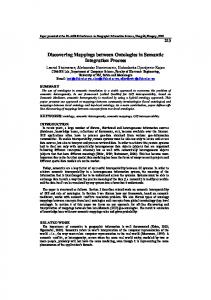
The way in which a Hilbert Curve is drawn is discussed in more detail in Lawder [4]. An insight, however, is rapidly gained from Fig. 1 showing the first 3 steps of an infinite process for the 2-dimensional case. A square is initially divided into 4 sub-squares which are then ordered such that any pair of consecutive sub-squares share a common edge. The ordering is illustrated by drawing a line through their centre-points and this line is called a first-order curve. Figure 1(b) shows the next step in which each sub-square is then divided into 4 sub-squares. The sub-squares within the first and last squares of the first step are ordered differently to ensure the adjacency property is always preserved. 0

1

2

3

15

012

5 1

9

6

10

2 4

0

7

8

11

3

2

13

12

0

1

14

15

3

1 0

(a)

(b)

2 3

63

(c)

Fig. 1. Approximations of the Hilbert curve in 2 dimensions

In practical applications, the process can be terminated after k steps to produce an approximation of a space-filling curve of order k. This curve passes through 2kn sub-squares, the centre-points of which are regarded as points in a space of finite granularity. The Hilbert Curve manifests a useful property in which consecutively ordered points are adjacent to each other in space. Most previous work on the calculation of mappings is confined to the 2dimensional case and a review is given in Lawder’s PhD thesis [4]. Bially [1] describes a generic set of rules for constructing state diagrams for use in calculating mappings but these rules are incomplete, requiring a process of ‘trial and error’. Lawder’s thesis supplements and specializes Bially’s rules so that state diagrams can be constructed for the Hilbert curve without manual intervention. 2

However, the space requirements for state diagrams for the Hilbert Curve grow exponentially with the number of dimensions and so they are only useful in up to about 8 dimensions. Butz’ algorithm in effect descibes a particular Hilbert Curve for each value of n. That more than one Hilbert Curve can be drawn through any space is readily illustrated by inverting the diagrams in Fig. 1.

3

Butz’ Algorithm for Mapping from a Hilbert derived-key to the Coordinates of a Point

In this section, we reproduce the algorithm for mapping from a Hilbert derivedkey to the coordinates of a point, given by Butz in [2]. Butz’ algorithm is iterative, requiring a number of iterations equal to the order of the curve. Butz summarizes the algorithm in two tables. The first, given here in Table 1, lists working variables and specifies how they are assigned values. These variables are ordered in the sequence in which their values are calculated, and new values are assigned within each iteration of the algorithm. With the exception of the variable αi , information is not provided on their semantics in [2]. The second, given here in Table 2, provides an example of the calculation process. The tables make use of the following variables and terms defined in or inferred from the paper: n: the number of dimensions in a space. m: the order of the curve passing through a space. N : the number of bits in a derived-key, ie nm. i : the number of the iteration of the algorithm, in the range [1, . . . , m]. r : an N -bit binary Hilbert derived-key, expressed as a real number in the range [ 0, 1). byte: a word containing n bits. ρij : a binary digit in r, such that r = 0.ρ11 ρ12 · · · ρ1n ρ21 ρ22 · · · ρ2n ρ31 ρ32 · · · ρm n . Thus ρi represents the ith byte in r, such that ρi = ρi1 ρi2 · · · ρin . aj : a coordinate in dimension j of the point, ha1 , a2 , · · · , an i whose derived-key is r. A coordinate is also expressed as a real number in the range [ 0, 1). αij : a binary digit in a coordinate aj , such that aj = α1j α2j · · · αm j . Thus in i i i i Table 1, α = α1 α2 · · · αn is an n-bit Z order derived-key formed from the ith bits of all of the coordinates in the point ha1 , a2 , · · · , an i. principal position: the last, or least significant, bit position, j, in ρi such that ρij 6= ρin . If all bits in ρi are equal, the principal position is the nth, or least significant. The most significant bit position is considered to occupy poistion 1. parity: the number of bits in a byte which are set to 1.

3

TABLE I Entities Used in Space-filling Curve Algorithm

Ji : An integer between 1 and n equal to the subscript of the principal position of ρi . In the following four examples of ρi for the case n = 5, the values of Ji are 5, 2, 4 and 5, respectively (the principal positions are circled): 1 1 0 0

1 1 1 1i 0i 111 0 1 1i 0 0 0 0 0i

σ i : A byte of n bits, such that σ1i = ρi1 , σ2i = ρi2 ⊕ ρi1 , σ3i = ρi3 ⊕ ρi2 , · · · , σni = ρin ⊕ ρin−1 , where ⊕ stands for the EXCLUSIVE-OR operation. τ i : A byte of n bits obtained by complementing σ i in the nth position and then, if and only if the resulting byte is of odd parity, complementing in the principal position. Hence, τ i is always of even parity. Note that the parity of σ i is given by the bit ρin and that a mask for performing the second complementation may be set up in the same process which calculates Ji . σ ˜ i : A byte of n bits obtained by shifting σ i right circular a number of positions equal to (J1 − 1) + (J2 − 1) + · · · + (Ji−1 − 1) There is no shift in σ 1 . τ˜ : A byte of n bits obtained by shifting τ i in exactly the same way. ω i : A byte of n bits where i

ω1 = 0 0 · · · 0 0

ω i = ω i−1 ⊕ τ˜i−1 ,

and where ⊕ indicates the EXCLUSIVE-OR operation on corresponding bits. αi : A byte of n bits where αi = ω i ⊕ σ ˜i. Table 1. ‘TABLE I’ from [2]

4

TABLE II Example of Calculation of a from r

n=5 m=4 N = 20 r = 0.10011000100010111000 i ρi Ji σi τi σ ˜i τ˜i ωi αi

1 100 3 110 110 110 110 000 110

2 11000 4 10000 11000 10110 11000 00110 10000

3 10001 4 11001 00001 00001 00001 11110 11111

a1 a2 a3 a4 a5

= 0.1010 = 0.1011 = 0.0011 = 0.1101 = 0.0101

4 01110 2 11101 10111 11100 10101 11111 00011

Table 2. ‘TABLE II’ from [2]

5

5 00000 5 00000 01000 10000 11000 01010 11010

00 0 0 0 0 1 1

0 0 0 0 0 0

4

Some Improvements to the Algorithm Given in Table 1

The improvements described in this section emerged from insights gained in specializing Bially’s rules for producing generator tables from which state diagrams are produced to facilitate Hilbert Curve mappings, as described by Lawder [4]. Calculation of σ i : The variable σ i is derived directly from the value of ρi . A close inspection of the definition of the former shows that it is the Gray-code1 of ρi . Thus σ i may be defined in a single operation rather than in n steps as indicated in Butz’ paper: σ i ⇐ ρi ⊕ ρi /2 where ⊕ denotes the exclusive-or operation. Calculation of τ i : In describing how the value of the variable τ i is determined, Butz notes that the result is always of ‘even parity’, by which is meant that it contains an even number of non-zero bits. We observe from the state diagram generator tables produced in the manner described by Lawder [4] that this characteristic is shared, specifically and only, by the first of a pair of column X2 values appearing in any row. Column X2 values encapsulate the coordinates of the first and last points on a first order curve which ‘replaces’ a point on some first order curve when it is transformed into a second order curve. This leads to the conjecture that there is a correspondence between these two values and this is supported by the results of experiments. Thus we are able to calculate values for τ i simply, in accordance with the method for calculating the first of a pair of column X2 entries described in [4]. This is detailed in Algorithm 1.

Algorithm 1 Simplified Calculation of τ i in Butz’ Algorithm 1: if ρi < 3 then 2: τi ⇐ 0 3: else 4: if ρi % 2 then 5: τ i ⇐ (ρi − 1) ⊕ (ρi − 1)/2 6: else 7: τ i ⇐ (ρi − 2) ⊕ (ρi − 2)/2 8: end if 9: end if

The calculations for other variables in Butz’ algorithm are performed in our implementation in accordance with Table 1. 1

The Gray-code sequence is a sequence of binary numbers in which any two successive numbers differ in value in one bit position only. They are discussed in more detail by Reingold et al [6].

6

5

Procedure for Mapping from the Coordinates of a Point to a Hilbert derived-key

Butz does not give an algorithm for mapping from the coordinates of a point to its Hilbert derived-key. We therefore give the algorithm in Table 3, presented in the same format as used by Butz. The values of variables Ji , τ i and ω i are calculated in the same way as described in Table 1. All other variables are calculated differently.

αi : A byte of n bits, such that αi1 = ai1 , αi2 = ai2 , · · · αin = ain . ω i : A byte of n bits where ω1 = 0 0 · · · 0 0

ω i = ω i−1 ⊕ τ˜i−1 , and where ⊕ indicates the σ ˜ i : A byte of n bits where

EXCLUSIVE-OR

σ ˜ i = αi ⊕ ω i ,

operation on corresponding bits.

σ ˜ 1 = α1

σ i : A byte of n bits obtained by shifting σ ˜ i left circular a number of positions equal to (J1 − 1) + (J2 − 1) + · · · + (Ji−1 − 1)

i

ρ: Ji : τ i:

τ˜i :

There is no shift in σ ˜ 1. A byte of n bits, such that ρi1 = σ1i , ρi2 = σ2i ⊕ ρi1 , ρi3 = σ3i ⊕ ρi2 , · · · , ρin = σni ⊕ ρin−1 , where ⊕ stands for the EXCLUSIVE-OR operation. An integer between 1 and n equal to the subscript of the principal position of ρi . A byte of n bits obtained by complementing σ i in the nth position and then, if and only if the resulting byte is of odd parity, complementing in the principal position. Hence, τ i is always of even parity. Note that the parity of σ i is given by the bit ρin and that a mask for performing the second complementation may be set up in the same process which calculates Ji . A byte of n bits derived from τ i in the same way that σ i is derived from σ ˜i.

Table 3. Entities used in the algorithm for mapping from the coordinates of a point to a Hilbert derived-key

7

6

Source Code for the Mapping Algorithms

In this section we implement the algorithms given in sections 3 and 5 in the C programming language. The correspondence between terms defined in section 3 and variable names used in the source code is summarized in Table 4. Butz’ Term Program Variable Ji J (J1 − 1) + · · · + (Ji−1 − 1) xJ ρi P σi S σ ˜i tS τi T τ˜i tT ωi W αi A Table 4. Key to Variables

/* This code assumes the following: The macro ORDER corresponds to the order of curve and is 32, thus coordinates of points are 32 bit values. A U_int should be a 32 bit unsigned integer. The macro DIM corresponds to the number of dimensions in a space. The derived-key of a Point is stored in an Hcode which is an array of U_int. The bottom bit of a derived-key is held in the bottom bit of the hcode[0] element of an Hcode and the top bit of a derived-key is held in the top bit of the hcode[DIM-1] element of and Hcode. g_mask is a global array of masks which helps simplyfy some calculations - it has DIM elements. In each element, only one bit is zeo valued - the top bit in element no. 0 and the bottom bit in element no. (DIM - 1). eg. #if DIM == 5 const U_int g_mask[] = {16, 8, 4, 2, 1}; #endif #if DIM == 6 const U_int g_mask[] = {32, 16, 8, 4, 2, 1}; #endif etc... */ #define DIM 3 typedef unsigned int #define ORDER

U_int;

32

typedef struct { U_int hcode[DIM]; }Hcode; typedef Hcode Point;

8

/*===========================================================*/ /* calc_P */ /*===========================================================*/ U_int calc_P (int i, Hcode H) { int element; U_int P, temp1, temp2; element = i / ORDER; P = H.hcode[element]; if (i % ORDER > ORDER - DIM) { temp1 = H.hcode[element + 1]; P >>= i % ORDER; temp1 = i % ORDER; /* P is a DIM bit hcode */ /* the & masks out spurious highbit values */ #if DIM < ORDER P &= (1 > 1) & g_mask[i]) P |= g_mask[i]; return P; } /*===========================================================*/ /* calc_J */ /*===========================================================*/ U_int calc_J (U_int P) { int i; U_int J; J = DIM; for (i = 1; i < DIM; i++) if ((P >> i & 1) == (P & 1)) continue; else break; if (i != DIM) J -= i; return J; }

9

/*===========================================================*/ /* calc_T */ /*===========================================================*/ U_int calc_T (U_int P) { if (P < 3) return 0; if (P % 2) return (P - 1) ^ (P - 1) / 2; return (P - 2) ^ (P - 2) / 2; } /*===========================================================*/ /* calc_tS_tT */ /*===========================================================*/ U_int calc_tS_tT(U_int xJ, U_int val) { U_int retval, temp1, temp2; retval = val; if (xJ % DIM != 0) { temp1 = val >> xJ % DIM; temp2 = val =1, j--) if (P & 1) pt.hcode[j] |= mask; for (i -= DIM, mask >>= 1; i >=0; i -= DIM, mask >>= 1) { P = calc_P(i, H); S = P ^ P / 2; tS = calc_tS_tT(xJ, S); W ^= tT; A = W ^ tS; /*--- distrib bits to coords ---*/ for (j = DIM - 1; A > 0; A >>=1, j--) if (A & 1) pt.hcode[j] |= mask; if (i > 0) { T = calc_T(P); tT = calc_tS_tT(xJ, T); J = calc_J(P); xJ += J - 1; } } return pt; }

11

/*===========================================================*/ /* H_encode */ /*===========================================================*/ /* For mapping from DIM dimensions to one dimension */ Hcode H_encode(Point pt) { U_int mask = (U_int)1 ORDER - DIM) { h.hcode[element] |= P > ORDER - i % ORDER; } else h.hcode[element] |= P >= 1; i >=0; i -= DIM, mask >>= 1) { for (j = A = 0; j < DIM; j++) if (pt.hcode[j] & mask) A |= g_mask[j]; W ^= tT; tS = A ^ W; S = calc_tS_tT(xJ, tS); P = calc_P2(S); /* add in DIM bits to hcode */ element = i / ORDER; if (i % ORDER > ORDER - DIM) { h.hcode[element] |= P > ORDER - i % ORDER; } else h.hcode[element] |= P 0) { T = calc_T(P); tT = calc_tS_tT(xJ, T); J = calc_J(P); xJ += J - 1; } } return h; }

12

References 1. Theodore Bially. Space-Filling Curves: Their Generation and Their Application to Bandwidth Reduction. IEEE Transactions on Information Theory, IT-15(6):658– 664, Nov 1969. 2. Arthur R. Butz. Alternative Algorithm for Hilbert’s Space-Filling Curve. IEEE Transactions on Computers, 20:424–426, April 1971. 3. David Hilbert. Ueber stetige Abbildung einer Linie auf ein Flachenstuck. Mathematische Annalen. 38:459–460, 1891. 4. Jonathan Lawder. The Application of Space-Filling Curves to the Storage and Retrieval of Multi-dimensional Data. PhD Thesis, Birkbeck College, University of London, 2000. 5. Giuseppe Peano. Sur une courbe, qui remplit toute une aire plane (On a curve which completely fills a planar region). Mathematische Annalen, 36:157–160, 1890. 6. E.M. Reingold and J. Nievergelt and N. Deo. Combinatorial Algorithms: Theory and Practice. Prentice Hall, 1977.

13