The application we consider in this work is that of camera pointing, but it is worth noting .... a large microphone array that spreads throughout the room is beneficial. .... In other words, the EMA prediction, pt, at time t is calculated with ..... where μp, σp are the mean and standard deviation of Rp over a fixed bounded range of τ, ...
18 Camera Pointing with Coordinate-Free Localization and Tracking Evan Ettinger1 and Yoav Freund2 2 Department
1 Google
Inc., Mountain View, CA of Computer Science and Engineering, UC San Diego, La Jolla, CA USA
1. Introduction In this work we consider the problem of using audio localization techniques to locate human speakers and point a pan-tilt-zoom (PTZ) camera in their direction. We study this problem in the context of the The Automatic Cameraman (TAC) - an interactive display installation at UC San Diego (Cheamanunkul et al., 2009). A frontal view of TAC is given in Figure 1. TAC is a system which gives the user a hands-free interactive experience through computer vision and audio signal processing technologies. To start the interaction a user must first approach the display and speak. The system then localizes where the speaker is via a microphone array, and directs the camera to point there. In this work we describe exactly this initial part of the system, namely, how to point the camera at sound sources accurately and reliably. The main novelty of our method is that it does not rely on a-priori knowledge of the position of the microphones and the camera and the orientation of the PTZ camera. Traditional methods for audio localization require specifying these positions and orientations within a coordinate system. We call our method coordinate-free as it does not require a-priori specified coordinate system nor does it attempt to construct one. Instead, in this work we take a statistical approach based on machine learning. Our algorithm analyzes the relationships between different measurements and deduces the mapping from microphone delays to pan/tilt angles required to point the camera towards the speaker. The ability to calibrate the system after deployment allows placing the microphones far from each other and with no pre-specified geometry. This, in turn, allows the user to optimize the locations of the microphone according to the acoustics of the particular location. The application we consider in this work is that of camera pointing, but it is worth noting that our method is not constrained to just this problem alone. Direction of arrival (DOA) estimation is used widely throughout robotics, general sonar applications, beam-forming, and many other domains. Our method applies when knowledge of a precise coordinate system isn’t needed, such as pointing a camera at an object, pointing a robot at an object, or simply estimating direction or arrivals relative to a reference point. The key observation behind audio localization techniques is that spatially separated microphones observe a time-delay between the arrival of a sound source. This is depicted in Figure 2. Estimating these time-delays accurately is a fundamental step in many popular
318
Advances in Sound Localization
localization techniques. In the next section, we briefly discuss how to estimate these time-delays which will be a fundamental underpinning of our coordinate-free methodology that follows. We first describe our technique based on statistical regression to map time-delay information from a frame of audio to a pan-tilt directive for our PTZ camera. This gives a method for estimating from a single frame of audio what direction the sound source is coming from. However, this method analyzes each time frame independently and does not leverage any temporal information, such as the ways speakers move in space. To address this temporal concern, we introduce a coordinate-free tracking methodology for estimating these time-delays accurately based on a particle filtering approach. We show that a naive implementation of a particle filter does not track these time-delays accurately. Instead, we propose two methods to improve the particle filter for this particular problem. The first is a manifold learning step that learns the low-dimensional structure on which these time-delays live. The second is a new particle filtering framework based on new advances in the online learning community that has several advantages over a traditional approach. We outline the details of these methods and discuss them in more depth in what follows. The rest of the chapter is organized as follows. In Section 2 we describe the fundamental concepts of the TDOA and the PHAT transform. In Section 3 we discuss traditional coordinate-based methods for localizing a sound source from time-delay estimates. In Section 4 we discuss our coordinate free approach that attempts to learn a regressor that maps time-delay information directly into pan-tilt directives for the PTZ camera. We show that our method lends to an accurate camera pointing method with experiments in Section 5. The system used in these experiments does not take into account noise in the TDOA estimates or information about the way humans move. In Section 6 we present a coordinate-free tracking method which takes this information into account. In Section 7 we describe experiments that demonstrate the improvement in performance that result from incorporating tracking into our system. We conclude the chapter with some final remarks.
2. Time-delay estimation The basis of sound source localization is that spatially separated pairs of microphones experience a time-delay of arrival from a fixed sound. An illustration of this physical phenomenon in a 2-d setting is shown in Figure 2. In this work we do not assume any knowledge of microphone or camera positions, however, for the expository discussion in this section it is useful to assume they are known and fixed. Let mi ∈ R3 be the three dimensional Cartesian coordinates for microphone i. For a sound source located at position s and assuming a spherical propagation model, the direct path time delay between microphone i and j can be calculated as Δij =
� m i − s �2 − � m j − s �2 c
(1)
where c is the speed of sound in the medium. Δij is often called the time delay of arrival (TDOA) between microphone i and j. It is worth noting that if f is the sampling rate being used, then the largest the TDOA can be in terms of audio samples is M = �mi − m j �2 f /c. In other words, Δij is always in the range [− M, M] and in practice can only be estimated to the nearest sample. This observation directly reveals the fact that close together microphones cannot have as wide a range of TDOAs as microphones that are spaced further apart. Placing microphones further
Camera Pointing with Coordinate-Free Localization and Tracking
319
Fig. 1. Frontal view of TAC display unit. PTZ camera and four of the seven total microphone are visible.
��
��
�� ���� ��
�
Fig. 2. Left: A 2-dimensional world with 4 microphones. Time-delay Δ12 is shown between microphones m1 and m2 . The sound source (red star) is shown with 2 degrees of freedom for movement (red arrows). Right: Suppose we restrict our view to the TDOA values Δ12 , Δ23 and Δ34 . The right hand side figure depicts the 2-dimensional manifold created by mapping locations in the 2-dimensional world to these three TDOA variables. The manifold is not affine because of the non-linearities of the geometry. However it is locally affine.Thus the red movement arrows of the figure on the left map to the red arrows of the figure on the right. apart allows for more variability in the feasible TDOAs, and hence, results in a better ability to discriminate between audio source locations in space. Given k microphones there are (2k ) unique pairs of microphones for which Δij can be estimated. k We let �Δ = (Δij )i< j ∈ R(2) be the vector that contains each of these unique TDOAs for a given
audio source location. We will often call �Δ the TDOA vector. When given a fixed Δij for a pair of microphones, we can deduce from Equation 1 that the set of feasible s positions that could have resulted in the observed Δij form one sheet of a 3-d hyperboloid in space (for a 2-d world representation see Figure 3). It follows that for a fixed
320
Advances in Sound Localization
�����������
�
���
Fig. 3. A 2-d world where 3 microphones are necessary to uniquely determine a sound source’s location via multilateration. If given Δ12 , Δ23 and knowledge of the microphone positions, then one can solve for the intersection of the corresponding hyperbolas for s.
�Δ, the possible audio source locations that could have generated such a TDOA vector can be determined through finding the intersection among all such hyperboloids. This procedure is known as multilateration. However, in practice we can only estimate each Δij from the underlying audio signals. As a result, the estimation procedure faces multiple challenges that easily lead to inaccuracies. First and foremost, sound easily bounces off of many physical materials causing multi-path reflections and reverberations. Secondly, the audio signal is only captured at a finite precision with respect to time since the signal must be digitized with a finite sampling rate. This means we can only estimate TDOAs with a finite precision that depends on the audio sampling rate. These challenges often results in estimation errors in Δij and so it is not surprising that in practice the intersection of all the corresponding hyperboloids is empty! One of the most popular time delay estimation (TDE) techniques, and the method used in this work, is a generalized cross-correlation (GCC) technique that utilizes the phase transform (PHAT), first discussed in the audio localization literature by Knapp and Carter and then further analyzed by many others (Knapp & Carter, 1976; Omologo & Svaizer, 1994; 1996). PHAT is very robust to noise and reverberations compared to other correlation based TDE techniques (J. DiBiase, 2001; Svaizer et al., 1997). Let Xk (ω ) be the Fourier transform of microphone k. The GCC between microphone l and m is Rlm (τ ) =
�
∞ 1 ∗ Ψ ( ω ) Xl ( ω ) Xm (ω )e jωτ dω 2π −∞
(2)
where Ψ(ω ) is a weighting function for the GCC and ∗ denotes complex conjugation. The PHAT weighting of the GCC is of the form Ψ(ω ) =
1 ∗ ( ω )| | Xl ( ω ) Xm
(3)
The PHAT weighting has a whitening effect by removing amplitude information in the signals. Compared to standard cross-correlation, PHAT puts all the emphasis on aligning the phase component of the transformed audio signals and none on the amplitudes. Empirically, it has been observed that the result of using the PHAT weighting is often a large spike in the GCC at the true TDOA. Hence the PHAT method for TDOA estimation is to let Δij = arg max Rij (s) s
(4)
Camera Pointing with Coordinate-Free Localization and Tracking
321
The PHAT correlations are typically very pronounced at the estimated TDOA with a small number of significant secondary peaks. It has been observed often that if the true TDOA is not at the largest peak it is often at one of these large secondary peaks (J. DiBiase, 2001). This property has been exploited by many methods, and will be exploited by the particle filtering method that we describe later on.
3. Related work Sound localization techniques via microphone arrays can be divided into two major paradigms: TDOA two step localization and steered response power (SRP) based. The first technique involves first estimating for a frame of audio the TDOAs between all pairs of microphones and then solving the subsequent geometric multilateration problem. The most popular is a least squares approach to find the 3-d location that is close to all the resulting hyperboloids. One such approach is to simplify the nonlinear least squares problem by linearizing it through either a Taylor expansion (Foy, 1976) or by introducing an extra variable as a function of the source location (Chan & Ho, 1994; Friedlander, 1987; Gillette & Silverman, 2008; Huang et al., 2001; Smith & Abel, 1987; Stoica & Li, 2006). This leads to a closed-form solution to the problem since it becomes a linear least-squares problem, but the resulting variance in the source location estimator is large (Chan & Ho, 1994; Huang et al., 2001). There are many other variations on this approach that could fall in this category as well (Brandstein et al., 1995; Gustafsson & Gunnarsson, 2003; Silverman et al., 2005). The second category for source localization techniques are all based on maximizing the steered response power (SRP) of a beamformer (J. DiBiase, 2001). For example, a simple instance in this class is to maximize the energy of a delay-and-sum beamformer over a range of steering directions. That is, for each source location x, one first calculates the corresponding TDOA vector, Δ( x ), derived from the array geometry. By delaying the frames of audio by these TDOAs and summing all the signals together, one gets a reconstruction of the original signal. This reconstruction has the most energy when Δ( x ) is correct. Conversely, Δ( x ) can be estimated by maximizing the energy of the reconstructed signal. Probably the most popular of SRP based beamformers is the so called SRP-PHAT beamformer (Do et al., 2007; J. DiBiase, 2001). Here, instead of maximizing the energy of the delay-and-sum reconstruction, one calculates the PHAT correlation, Rij (τ ), for all pairs of microphones and then solves the optimization arg maxx ∑i< j Rij (Δij ( x )). Both the two step and beamforming based methods require knowledge of a coordinate system wherein microphone positions are known. For small microphone arrays a coordinate system can easily be found by simply measuring the distances between microphones by hand as in (Wang & Chu, 1997). If we want to be able to localize sounds in a large room accurately, then a large microphone array that spreads throughout the room is beneficial. However, measuring accurately by hand the relative distances now becomes much more difficult and positional errors on the order of 1-5cm can seriously degrade beamforming techniques (Sachar et al., 2005). Since doing such measurements is often too difficult, especially for arrays with many elements, many techniques have been developed to automatically calibrate the positions of the microphone elements (Birchfield & Subramanya, 2005; Hörster et al., 2005; McCowan et al., 2008; Raykar & Duraiswami, 2004; Sachar et al., 2005). These techniques are based on using a carefully designed device that emits a special sound. Delay measurements are made at the array and with the known geometry of the device one can solve for the microphone positions. Typically distances from the device to the microphones, or inter-microphone
322
Advances in Sound Localization
distances are estimated. For example, if pairwise distances between microphones can be estimated, then multidimensional scaling (MDS) can be used to find the location of the sound source (Birchfield & Subramanya, 2005; Hörster et al., 2005; McCowan et al., 2008; Raykar & Duraiswami, 2004; Sachar et al., 2005). Note that if we were to use a coordinate based system to estimate the location of the speaker we would need an additional step to map the estimated location to the direction directive for the PTZ camera. To compute this mapping we would need to know the location and orientation of the camera relative to the microphones. Instead we developed a coordinate free method which maps the estimated delays directly to pan and tilt commands for the camera. In this way we avoid the need to measure the relative locations of the microphones and the camera. In order to learn the mapping from delays to pan/tilt (PT) we collect observations consisting of a set of delays between microphones for a fixed source location and the associated PT to center such a source. With this database of samples, we estimate via regression analysis a model for the system. This model allows us to estimate for a fixed �Δ what the corresponding PT directive for our camera should be. We describe the methodology and experiments for this method in the next two sections.
4. Coordinate-free localization In this section we describe the regression models we use for estimating the mapping from �Δ to PT. For what follows assume that a training set of size m is given with observations of the form yi = (θi , ψi ), for pan and tilt respectively. These observations are paired with an estimated TDOA vector derived from the N microphones, namely xi = �Δi with p = ( N2 ) coordinates. We organize the training set into matrices Y ∈ R N ×2 and X ∈ R N × p where each observation is a row vector. In what follows, we briefly remind the reader of least squares linear regression and a tree based regressor based on principal direction trees (PD-Trees) (Verma et al., 2009). Least squares linear regression
For each column of Y, denoted Yi , we fit a separate linear regression model. The linear regression model has the form f (X ) = β0 +
p
∑ Xj β j
j =1
where X j is the jth column of X and β is the vector containing the coefficients in the linear model. The least squares (LS) solution to linear regression chooses the model that minimizes the residual sum of squares (RSS) RSS( β) =
N
∑ (yi − f (xi ))2
i =1
When X is full rank the LS solution can be written in closed form as β = ( X T X )−1 X T Yi . It is known that if the true model of data generation is linear, then the LS estimator is the minimum variance unbiased estimator of β.
Camera Pointing with Coordinate-Free Localization and Tracking
323
PD-tree
In the experiments described in the next section we will also explore the use of a constant depth PD-Tree with regressors learned in each leaf node. A PD-Tree is a binary partitioning tree that at each node projects the data present in that node onto its principal direction and splits the data into two children nodes based on the median value. We grow a PD-Tree to depth 2 and fit linear least squares regressors in each leaf node. This will act as a piece-wise regression model. Principal direction trees are chosen since they are known to adapt quickly to low dimensional structure present in data (Verma et al., 2009). We know that our TDOA data, despite being in rather high dimensions has a low dimensional structure since it has underpinnings to a physical location from the generating sound source. Sound sources only have 3 spatial dimensions in which they can vary so as a consequence our TDOAs also have exactly this many degrees of freedom. Although the underlying structure on which these TDOAs is not linear (intersection of hyperboloids), but is locally linear. As we shall see in the next section, a PD-tree of depth three yields a good approximation for most of the area covered by the automatic cameraman.
5. Experiments: Localization bias In this section we present two experiments. The first one generates a training set and test set with a simple device that helps us collect training examples. The second experiment aims to learn examples over time from people who interact with our display over time. We describe each in further detail in what follows. 5.1 Experiment: Grid dataset
The device used to collect all the data in the experiments to come is shown in Figure 4b. It consists of a simple radio and a green LED attached to a 9V battery with a switch and dimmer all in a plastic encasing. We will call this the calibration device from here on. The radio component of the calibration device can be tuned to a nonexistent station that emits noise that is very close to white. This random noise typically has the most consistent TDOA vector estimates using the PHAT technique. A simple color thresholding detector was written to find the LED in the camera’s field of view using Max/MSP and Jitter (Max/MSP website, n.d.). The result is a real-time control of the PTZ-camera to keep the LED centered in the field of view, and a constant white noise to calculate TDOAs for. The calibration device is used to collect samples of TDOA vectors in unison with where the camera is pointing to center the green LED in its field of view. The camera can be queried as to what the pan and tilt it is currently whenever a TDOA vector is collected. These two pieces of information are recorded together as a complete observation instance. The result of the training set collection is a dataset of close to 28k observations. We noticed that when a estimate for Δij was incorrect, it typically had a very large deviation from what was often consistent. To remove such noisy observations, we performed some simple outlier removal by thresholding the magnitudes of the �Δ projections onto the bottom global PCA eigenvectors (orthogonal space) leave approximately 20k observations remaining as our training set. We then did a PCA analysis of just the �Δ parts of this training set. Figure 4 shows the percentage of variance explained by the addition of each eigenvector. It’s clear that the top two eigenvectors dominate most of the variance explained, and that the 3rd eigenvector seems to have a significant advantage over the remaining ones. The total percent variation captured by the top 3 eigenvectors is nearly 90%. This follows from the fact that there are 3 spatial
324
Advances in Sound Localization
���
���
Fig. 4. Left: Percentage of variance explained by top X eigenvector. The top 3 eigenvectors dominate and the rest are noise. Right: Calibration device used to collect training and grid dataset. degrees of freedom that were examined during the training data collection period. Moreover, two of these spatial directions had much more spatial variance then the third, ceiling-to-floor, spatial direction. The room is simply much larger in width and breadth than the variance in observation heights, which matched typical heights that human speakers could appear at. From this training set with outliers removed we have nearly 20k observations with which we learn a simple linear least-squares regression (LS) model and a PD-Tree model of depth 2. We would like to analyze how the bias-variance trade-off of these simple models behaves as function of physical position of the sound source in the lobby. In other words, in what areas do these simple models perform well, and where does the inherent non-linearity of the problem cause large bias? With these questions in mind we collect a test set of data in a similar fashion to the training set. We place the calibration device at a fixed height (approximately 1m from the floor) and roll it along straight lines using a rolling chair. We repeat this process for each of the 13 lines in the grid depicted in Figure 5b. This results in a variety of observations that cover a representative set of the spatial variability in the room relevant for human speakers. Moreover, using white noise as our sound source will simulate the behavior of our model under conditions where TDE is highly optimized. This gives us insight into isolating the effects of the model assumptions. Figure 5a depicts the embedding of the TDOA vector components of the entire grid test set onto the top 2 eigenvectors from the PCA learned from the training set. The zoomed in portion depicts lines 9-13 in red and lines 1-6 in blue in the same orientation as the diagram in Figure 5b. The curved nature of each line can be observed from such plots. Even though the spatial location of the sound source is varying along a straight line in space, the corresponding location in the TDOA vector space corresponds to slightly curved trajectories. It is clear that a linear model for spatial location is not going to fully capture all the variation, but nevertheless the grid structure is still very recognizable in even just the top 2 eigenvectors indicating that a linear model is a good approximation in these regions. Figure 5c compares the predictions from the simple linear LS model to the pan and tilt recorded from the light detector. The dots in black are the predicted pan (or tilt) from the model for each TDOA vector observation. The green line depicts the pan (or tilt) from the light detector. Finally the red line depicts an exponential moving average (EMA) of the model predictions over time. In other words, the EMA prediction, pt , at time t is calculated with
Camera Pointing with Coordinate-Free Localization and Tracking
325
Fig. 5. (a) Embedding of the TDOAs collected from the grid onto top 2 eigenvectors. The entire embedding is shown small in the upper right corner and a zoomed in portion of the same embedding is shown larger. (b) To the right is a diagram of the equispaced grid over which data was collected. (c) Below are 3 selected lines and the LS predicted value for each TDOA collected. Also depicted in red is an exponential moving average of the predictions (α = 0.10), and in green where the camera was pointing to center the LED.
326
Advances in Sound Localization Model
1 4.31 4.22 5.15 4.70
LS-pan PD-pan LS-tilt PD-tilt
Grid Line Number 5 7 9 2.22 5.99 3.56 3.05 4.14 3.05 7.50 3.33 5.63 4.65 3.26 4.82
3 2.77 3.14 7.57 4.72
11 3.20 2.45 3.90 2.95
13 3.96 3.88 4.48 6.55
avg 3.87 3.47 5.75 4.55
Table 1. RMSE (in degrees) of different regression models for each grid line. RMSE of TAC 8
Pan RMSE Tilt RMSE 90th Perc. Pan RMSE 90th Perc. Tilt RMSE
7
RMSE (in degrees)
6
5
4
3
2
1
0
2
3
4
5
6
7
8
9
10 11 12 13 14 15 16 17 18 19 20 21 22
Week Number
Fig. 6. RMSE for pan and tilt of a PDTree trained each week with new data acquired by TAC. update pt = (1 − α) pt−1 + α f (Δt ), where f (Δt ) is the prediction of the raw observation at time t. We chose α = 0.1. The EMA line should give us a sense of what the true model predictions are by smoothing out the observation noise. In doing so, we can compare the light detector observations to the EMA line and get a sense for the bias in our model. Table 1 gives the root-mean squared error (RMSE) between the EMA of the model predictions and the observations from the light detector for each of the regression models. The PD-Tree method outperforms a simple linear model. Moreover, the overall averages are very similar to results reported by traditional coordinate based methods, meaning that coordinate-free methods need not sacrifice accuracy (Badali et al., 2009). 5.2 Lifelong learning
We can easily acquire a training set without the aide of a device with help from a face detector. Training examples can be collected whenever a user speaks while their face is centered in the field of view, creating a stable measurement of the form (�Δ, θ, φ). Many such examples can be collected over time by having the PTZ-camera continually centering the user’s face and the user continuing to speak. This is in fact what we do in TAC. Whenever a user is interacting with TAC a log is recorded that records these stable training points. We retrain a PDTree with linear models in the leaves at the end of each week on the entire training set collected up to that point. We took all the observations TAC has seen over a period of approximately 6 months (∼3000 observations), and split this randomly into a 70/30 training and test set. We then examined how TAC can improve its localization accuracy by retraining a regressor for pan and tilt each week on the data from the training set seen to that point. We averaged root-mean squared
Camera Pointing with Coordinate-Free Localization and Tracking
327
error (RMSE) calculations over 20 such random training/test splits. Figure 6 shows the improvement of this regressor in terms of RMSE. Also shown is the RMSE when the top 10% of squared-residuals are removed from the RMSE calculation. The improvement is near-linear from week to week. Moreover, many of the errors are near or below one degree in both pan and tilt. This is promising since the locations in the test set are representative of where most users frequent when interacting with TAC. This means we are very accurate (< 1 degree error) in these locations.
6. Coordinate-free TDOA tracking One deficiency of the methods presented thus far is that the are frame based methods that do not leverage temporal information. For instance, we know that sound sources do not move quickly or disappear and reappear in different locations instantaneously. Therefore, some smoothness assumptions about the variability of TDOAs over time would be beneficial to a general methodology that attempts to localize sound sources using information across many frames. In TAC we have 7 microphones, causing a 21-D TDOA vector. In what follows we propose a particle filtering methodology for tracking the 21-D TDOA vector over sequential frames of audio. The methodology has three important innovations above the naive median filtering strategy outlined above. The first is that TDOAs from one frame to the next should not vary too much. This assumption should be explicitly integrated into any model of tracking. A second observation is that TDOAs can only occur from a feasible region of the 21-D space in which TDOA vectors lie. We propose a PD-Tree based model of this feasible region. It is well known that particle filters tend to break-down when the object being tracked have many dimensions to their state space. By modeling the feasible region, we alleviate this well known deficiency of particle filters by making the effective dimensionality of the TDOA space much lower. The last contribution is a new particle weighting and resampling scheme inspired by results in online learning. The resampling scheme is such that we can leverage the PD-Tree model in a novel fashion that allows for averaging over different bandwidths in the tree. We will show in the experiments that this averaging scheme can improve over baseline schemes especially when a sound source enters regions that are not modeled well by a single global linear model. In addition, it is known that the weighting scheme used is much more robust to model mis-specification than traditional particle filters. 6.1 Particle filters
Particle filtering is an approximation technique used to solve the Bayesian filtering problem for state space tracking (Arulampalam et al., 2002). More specifically, assume we have observations yt and a state space xt . Often the state space will consist of the position of the object of interest, and sometimes higher moments like velocity or acceleration. The goal of the particle filter is to keep a discrete set of particles that well-approximates the posterior density of the current state given the past observations p( xt |y0 , . . . , yt ). In the TDOA tracking problem our observations yt will be the PHAT correlations for a given frame of audio and the state space xt will be composed of each of the D = (2k ) time delays. The bootstrap is one of the most popular particle filtering algorithms (Gordon et al., 1993). (i )
Here, a weighting over m particles is chosen to approximate the posterior density. Let wt
328
Advances in Sound Localization
be the weight associated with particle i at time t. Then, a single iteration of the algorithm proceeds as follows: (i )
1. Sample: draw m particles xt−1 from the existing set of particles according to their weights (i ) w t −1 .
(i )
2. Propagate: Let the particles propagate according to the transition function, xt (i ) g ( x t −1 ) + u t .
(i )
(i )
=
(i )
3. Weight update: Update weights according to wt = wt−1 p(yt | xt ) and normalize so they sum to one. The result is a set of particles approximately distributed as the posterior density p( xt |y1:t ). This sample set allows for computation of any quantity as a function of the posterior. For example, often we would like to estimate the mean of the posterior distribution which will be our prediction of the current state. This estimate is given by xˆ t =
�
xt p( xt |y1:t )dxt ≈
m
(i ) (i ) xt
∑ wt
i =1
(5)
The weights are chosen to approximate the relative posterior density for their respective particles. This popular variant of particle filters has been shown to perform well in the coordinate-based tracking literature (Lehmann & Johansson, 2007). The key decisions for optimizing such a particle filtering algorithm are: 1. Likelihood: The choice of likelihood function, p(yt | xt ), is critical since this will govern how weights are calculated. 2. Propagation function: The propagation function g(·) is also essential and needs to be chosen accurately. In coordinate based methods g is chosen to be linear and uk often to be Gaussian. 3. Number of particles: The total number of particles m. The larger m is the more computational load the system must undertake. Optimizing m is of paramount importance for real-time implementations. More so than the other choices, the likelihood function is by far the most difficult. The true likelihood function for how PHAT observations are generated from a given sound source location seems very difficult to model. Nevertheless, it has been shown that some simple choices for the likelihood function can lead to good tracking performance (Lehmann & Johansson, 2007). In making a choice for the likelihood function, first notice that we must have support over the entire observation space. If we don’t meet this requirement, particles that occur with likelihood zero will get weight zero and die immediately. This is not the behavior we would like since particles that were performing well in the past may then suddenly die. Instead, we should want a more graceful way for particles to tend towards zero weight. As a result, often a mixture of a uniform prior over the entire observation space is mixed with the likelihood function to avoid this behavior. One deficiency of the particle filter is that accurate tracking becomes very difficult when the state space becomes larger than a few positional locations (e.g. 2-D or 3-D locations). In TDOA tracking, the state spaces can potentially be much larger. For example, the seven microphones
329
Camera Pointing with Coordinate-Free Localization and Tracking
Algorithm 1 Generic bootstrap based particle filtering audio tracking algorithm. (i )
(i )
Initial Assumptions: At time t-1, we have the set of particles xt−1 and weights wt−1 , i ∈ {1, . . . , m}, being a discrete representation of the posterior p( xt−1 |y1:t−1 ). (i )
1: Dynamics: Propagate the particles through the transition equation xt
(i )
= g ( x t −1 , u t ). (i )
2: Weight Update: Assign each particle a likelihood weight according to wt
Then, normalize weights so that they sum to 1.
(i )
= p ( y t | x t ).
(i )
3: Resample: Resample m new particles from { xt }im=1 according to the weight distribution (i ) {wt }im=1 .
each.
(i )
Let these be the new set of particles { xt }im=1 and assign uniform weight to
in TAC give rise to a 21-D TDOA vector space, but with arrays with more microphones the space can be even larger. The difficulty arises in the randomness need in uk to generate enough variety of particles so that a few are close to a good state representation. One obvious remedy would be to increase the number of particles, but this causes the real-time feasibility of the algorithm to quickly diminish. To alleviate this problem, when a coordinate system is known, then the state space can be represented as the 3-d position of the audio source. This makes the algorithm feasible with a small number of particles (typically < 100). In our coordinate-free approach, we take a similar dimensionality reduction technique by directly modeling the low dimensional structure on which the TDOAs lie via a PD-Tree. However, before introducing our algorithm we first discuss related work in coordinate based TDOA tracking. 6.2 Related work
Particle filtering methods dominate the audio source tracking literature (Lehmann & Johansson, 2007; Li & Ser, 2010; Pertilä et al., 2008; Talantzis et al., 2009). The seminal work of Ward et. al is the first to popularize the use of particle filtering methods for audio tracking and is still widely regarded as state-of-the art (Ward et al., 2003). Further experiments and slight improvements on this method were presented in Lehmann & Johansson (2007). This method is the focus of what follows realizing that the others mentioned above are all derived from this seminal work. We reproduce the bootstrap particle filtering method for audio source tracking in Algorithm 1. (i ) (i )
The predicted state at each step of this algorithm is the weighted mean xˆ t = ∑im=1 wt xt . (i ) xt
Here the state space is chosen to be 3-d Cartesian coordinates = [ p x py pz ] and the dynamics g is chosen to be the identity with spherical Gaussian noise for uk . The size of the Gaussian noise uk is a tunable parameter that must coincide with the assumptions about how quickly the objects being tracked can move. The major choice in the algorithm is how to perform the weight update step, in particular, (i )
what choice should be made for the likelihood function p(yt | xt ). The choices for this function can arise either from GCC based methods or steered beamforming based methods. For example, a simple steered beamforming based approach is as follows. For the weight (i )
(i )
update in Algorithm 1, let p(yt | xt ) = F (yt , Δ( xt ) where F calculates the steered response (i )
power of the current frame of audio steered towards xt . More computationally efficient methods for representing the likelihood function were presented in Ward et al. (2003) based on PHAT transforms. The idea for the likelihood here is
330
Advances in Sound Localization
to define a function that combines how close the current particle is to the largest peaks in the PHAT correlation from each pair of microphones p ∈ {1, . . . , D }. This will be the method we use in the work presented in this chapter. In particular we use the following. First, to identify the peaks in a given pair’s PHAT function we take a simple z-scoring method. Let [ A]+ = max (0, A). Then, for each PHAT correlation R p let it undergo a z-scoring transform as follows (note from here on we drop the subscript t for ease of notation): � � R p (τ ) − μ p Z p (τ ) = −C (6) σp + where μ p , σp are the mean and standard deviation of R p over a fixed bounded range of τ, and C is a constant requiring that peaks be at least C standard deviations above the mean. This performs well to find a small, fixed number, of peaks K p in each R p . We now define p(y| x (i) ) in terms of these peaks: p ( y | x (i ) ) ∝ p0 +
D
Kp
∑ ∑ Zp (τl )N(τl ; Δ(x(i) ) p , σz2 )
(7)
p =1 l =1
where Δ( x (i) ) p the TDOA associated with pair p derived from the 3-D location x (i) , N ( x; μ, σ2 ) is the density under a normal distribution evaluated at x with mean μ and variance σ2 , and Z p has K p non-zero entries each of which are at τl . The parameter p0 is the background likelihood that determines how much likelihood is given to any TDOA regardless of the observation. This parameter is essential for this kind of particle filter so that the likelihood function never evaluates to 0. Otherwise a particle’s weight can never abruptly vanish. The variance parameter σz2 controls how much weighting is given relative to how far each state is from the peaks in the corresponding PHAT series. So, a particle will be given high likelihood if the particle’s derived TDOA matches well with the largest peaks in the observed PHAT series. Conversely, if the derived TDOA is far from any of the observed peaks it will be given a very low likelihood. A nice property of this choice of likelihood is that it does not rely solely on the maximum of each PHAT series being accurate (a similar advantage was observed between steered beamformers over the 2-step localization procedure discussed in previous sections). Since often the peaks in the PHAT localization are corrupted due to reverberations or multipath reflections, relying heavily on only these maximum peaks is not robust. The likelihood defined in Equation 7 neither relies too heavily on the accuracy of a single pair of microphones, nor on the largest peak in each pair’s PHAT series. Secondary peaks can contribute substantially to the likelihood as well. As we will see, integrating a particle filtering based tracking method into the localizer will lead to a much stabler and robust localization method. 6.3 Normal hedge based particle filter
In this section we introduce the Normal Hedge based particle filter. This particle filter, although very similar to the traditional particle filter introduced above, will have several advantages. First, the resampling scheme will not require particles to be resampled every iteration. In fact, particles will remain “alive” for as long as they perform well. Secondly, the requirements of the algorithm will allow for much more flexibility in specifying a likelihood function. Recall that in Equation 7 we had to define a parameter for the background likelihood p0 , otherwise particles could quickly go to zero weight and die. No such requirement is
Camera Pointing with Coordinate-Free Localization and Tracking
331
needed by the particle filter presented here, moreover, the guarantee that will be given is relative to the defined likelihood function. This means that the resulting Normal Hedge particle filtering algorithm will perform well as long as the likelihood function encourages good tracking performance (i.e. high likelihood scores indicate that the particle matches the observation well). Before introducing the full Normal Hedge particle filter we first discuss the Normal Hedge online algorithm for predicting from a group of experts’ advice, initially presented in Chaudhuri et al. (2009). Normal Hedge
The Normal Hedge algorithm is a parameter-free online algorithm for hedging over the predictions from a group of N experts (Chaudhuri et al., 2009). One of the barriers to practical implementations of previous online learning algorithms was that they all contained a learning parameter that was very important to tune correctly for good performance. Normal Hedge has no such parameter, yet still has a very strong performance guarantee like that of the previous online algorithms. The setup for the algorithm is as follows. At each iteration t expert i makes a prediction (i )
that has an associated loss �t ∈ [0, 1]. The notion of loss in this setting is very general, but in most cases is typically derived as a function of the expert’s prediction and the actual observation (e.g. the difference between the prediction and the observation normalized to the (i )
[0, 1] range). The algorithm maintains a discrete probability distribution over the experts wt . After observing the losses, the learner itself incurs a loss according to the expected loss under this discrete distribution, �tA =
N
(i ) (i ) �t
∑ wt
i =1
(8)
The notion of regret is the essential quantity of interest in online learning. The algorithm’s (i )
(i )
instantaneous regret is defined as rt = �tA − �t and the cumulative regret up to time t is defined as (i )
Rt =
t
(i )
∑ rτ
(9)
τ =1
Intuitively the cumulative regret measures how well the algorithm is doing relative to a single action chosen to predict at all previous iterations up to t. The goal for an online algorithm is to minimize the cumulative regret of the algorithm relative to any given expert (in particular, the best expert in hindsight). The Normal Hedge algorithm is given in Algorithm 2. It requires no parameters and the computational needs are also simple. The algorithm must maintain the weights and regrets over each of the N experts and also a line search is needed to solve for ct in the weight update stage. The guarantee proved in Chaudhuri et al. (2009) is that the cumulative regret to the best � percentile of experts will be small. In particular at time t the cumulative regret of Normal � Hedge to the � percentile expert will be O ( t(1 + ln 1/�) + ln2 N ). This is more general than the regret bounds that already existed in the online learning literature which only considered regret to the “best” expert in hindsight. The notion of “� percentile” is a more useful bound in the sense that in many practical situations there are many experts among the N which are almost as good as each other. As a result, guaranteeing performance relative to the
332
Advances in Sound Localization
Algorithm 2 Normal Hedge parameter-free online learning algorithm. (i )
Initial Assumptions: At time t − 1 we’re given the cumulative loss of each expert Rt−1 and (i ) (i ) (i ) the discrete weighting wt . Initially R0 = 0 and w1 = 1/N for all i. (i )
(i ) (i )
1: Update Losses: Each action incurs a loss �t
and the learner incurs loss �tA = ∑iN=1 wt �t . (i ) (i ) (i ) 2: Update Regrets: Update the cumulative regrets Rt = Rt−1 + (�tA − �t ) � (i ) � 2 ([ Rt ]+ ) 1 3: Update Weights: First, find ct > 0 that satisfies N = e. Then, update ∑iN=1 exp 2ct � � (i ) (i ) (i ) [ Rt ]+ ([ Rt ]+ )2 weight distribution for round t + 1 by wt+1 = exp . Normalize the ct 2ct weights so they sum to one. absolute best is often too strong. Moreover, the bound given in Chaudhuri et al. (2009) is still competitive with other known results when considering the “best” expert case by setting � = 1/N. NH-pf derivation
Transforming the Normal Hedge algorithm into a particle filtering algorithm is quite natural. We must only transform the terminology “experts” into “particles” and we’re most of the way towards a Normal Hedge based particle filtering algorithm. A recent paper was published that was that first to describe how the Normal Hedge algorithm can be used as a particle filter (Chaudhuri et al., 2010). In the tracking problem we consider an expert to be a predictor of a sequence of hidden states ( x1 , . . . , xt ) up to time t. This sequence of states is a proposed explanation for the sequence of observations (y1 , . . . , yt ). Instead of a likelihood function p(yt | xt ) like in particle filters, for the Normal Hedge tracking algorithm we must define a loss function on which to measure each (i )
expert’s performance. The loss �t for expert i should measure how well an experts sequence of states matches the sequence of observations. After defining this loss, we nearly have all the components needed to utilize Normal Hedge in the tracking framework. However, there is a computational issue at hand, namely, the exponential explosion in possibilities for state space sequences. Imagine we could run Normal Hedge over this enormous number of experts. Luckily, we’d have one advantage on our side because the Normal Hedge weighting would give many experts weight zero except for a core group that are outperforming the predictions of the algorithm itself. Nevertheless, some approximation is necessary, but this sparsity property will ease the requirements of any approximation. The approach we take will sample from this large set of experts in a very similar fashion to that of the bootstrap particle filter described earlier in this chapter. Just as the particles in a particle filter are a discrete approximation to the posterior density, we will utilize a set of particles to approximate the induced distribution by Normal Hedge over the set of state sequences. The Normal Hedge algorithm for TDOA tracking is given in Algorithm 3. Notice that a further simplification is taken to the problem by only maintaining the discounted cumulative regret (i )
(i )
(i )
Rt = (1 − α) Rt−1 + (�tA − �t )
(10)
where the parameter α controls how much memory our tracking algorithm should have in terms of penalizing losses observed in the past. This approximates the need for tracking
333
Camera Pointing with Coordinate-Free Localization and Tracking
Algorithm 3 Normal Hedge based particle filter. (i )
Initial Assumptions: At time t-1, we have the set of particles xt−1 and Normal Hedge weights (i ) w t −1 ,
i ∈ {1, . . . , m} (i )
1: Regret Update: Obtain losses �t (i ) Rt
(Equation 10).
(i )
2: Resample: For each particle xt
(k)
1. Choose a current particle xt (i )
for each particle and update discounted cumulative regrets (i )
with Rt < 0, resample a new particle in its place (i )
according to {wt }im=1 . (k)
2. Let the new particle xt = xt + uk , where uk is Gaussian noise. (Coordinate-free only): Project back onto the TDOA manifold using the PD-tree projection. (i )
(k)
3. Assign Rt = (1 − α) Rt
(i )
+ (�tA − �( xt )).
3: Weight Updates: Update the weights of each particle according to the Normal Hedge
procedure (see Algorithm 2). Normalize them to one.
(i )
4: Dynamics: Propagate the particles through the transition equation xt
(i )
= g ( x t −1 ).
sequences of states. Since typically we only want to predict the current state, this is an acceptable simplification. The weights can then be calculated according to the steps involved (i )
for computing wt
in the Normal Hedge algorithm (see Algorithm 2). What remains as a (i )
critical algorithmic choice is how we compute the loss �t for each particle, analogous to the decision of the likelihood function in particle filters. A nice property of this filter (NH-pf) is that the resampling procedure for particles emerges naturally from the Normal Hedge weighting function. A particle will be given zero weight whenever its cumulative regret has started to perform worse than the algorithm itself, and at this moment it is resampled near a particle that has good historical performance. Another nice property of NH-pf is that it can still maintain good tracking performance when the loss function has a modeling mismatch with the true observation process (Chaudhuri et al., 2010). Chaudhuri et. al show that if a traditional particle filter has a likelihood function that mismatches the true underlying process, then its performance will break down much quicker than the corresponding NH-pf. This final observation could prove to be advantageous in the TDOA tracking scenario. As stated earlier, choosing a likelihood function for TDOA tracking is somewhat arbitrary since the process for generating a PHAT observation from a given source location is extremely difficult to model. For this tracking problem and many other of practical importance, a model mismatch of this kind is unavoidable. TDOA tracking with coordinate-free NH-pf
We now describe how we track TDOAs in a coordinate-free fashion. First, we expand the state space to be that of the entire TDOA vector (for TAC a 21-dimensional state space). In addition, we must specify what loss function we will be using to calculate regrets relative to. We will utilize the negative likelihood function described in Equation 7 (i )
(i )
�t ( xt , yt ) = − p(yt | xt )
(11)
As discussed earlier, tracking in this many dimensions becomes difficult, but we also know that our TDOAs lie on a low dimensional manifold. In previous sections we discussed PD-Tree
334
Advances in Sound Localization
��
��
� ����� ��������� �� ��
� �� ��
����������� ��� ������� ��
���� ���������������� ����
Fig. 7. Depiction of a dead particle resampled and projected back onto the manifold. based regression models. We again utilize a PD-Tree to alleviate this high dimensional tracking problem, however, at the leaf nodes instead of a regressor we learn a low dimensional affine model via a PCA. During the resampling step for new particles, after noise is added to the newly born particle it is projected back onto the TDOA structure via the appropriate PCA model in the PD-Tree leaf node. This process is depicted in Figure 7. First, the corresponding leaf node for the newly born particle is found. Then, the particle is denoised by projecting it onto the principal components of local piece of the manifold stored within. The overall effect is a tracking algorithm that is constrained to have a state-space lie on the low dimensional structure captured by the PD-Tree. Note that there is a bias variance trade-off as you descend the PD-Tree in terms of the principle components models stored in each node. The nodes higher up in the tree have small variance since the bulk of the training data was used to learn the principal directions. However, the bias is also large at these nodes since a linear model is not appropriate at this granularity. As you descend the tree the variance increases, whereas the bias decreases as you approach locally linear regions. Moreover, the fit from individual nodes may vary across even their own partition region. Consider a given internal node of the PD-Tree. For a certain region of the cell’s partition the linear model may be a good fit, whereas in other regions of the cell’s partition it may be poor. It is clear from this argument that the best node that fits the true TDOA for a given source location will vary with location both across the tree and possibly in depth as well. It then makes sense to consider using the entire PD-Tree during the projection step instead of just the leaves at a fixed depth. A natural way to accomplish this emerges from the NH-pf resampling scheme by making a slight alteration to the projection step with the PD-Tree discussed above. After resampling a newly born particle and before projecting it back onto the manifold via the PD-Tree, first pick a depth uniformly at random in the PD-Tree. This will be the depth used for this single newly born particle, and this procedure is repeated for each newly born particle.
Camera Pointing with Coordinate-Free Localization and Tracking
335
This random strategy will have the nice property that it will naively find the correct model depth for the current sound source location over time. Depths that are chosen that are poor models will have particles die soon thereafter, whereas particles that are drawn from depths that perform well will survive. We will examine this procedure in the experiments that follow.
7. Experiments: TDOA tracking The experiments that follow were conducted from recordings of real speakers talking and moving slowly while facing TAC’s microphone array. We describe each individual experiment in detail in what follows. Setup
To build a PD-tree we first collected a training set of TDOA vectors from our microphone array. We accomplished this by moving a white noise producing sound source around the room near typical locations that sitting or standing people would be interacting with the display. This resulted in approximately 20,000 training TDOA vectors to which we built a PD-tree of depth 2. In each node of the PD-tree we store the mean of the training data and the top k = 3 principal directions. Here are the parameter settings we use for the experiments that follow. We use m = 50 particles for each type of particle filter examined. The discounting factor for NH is set to α = 0.05. We made several real audio recordings of a person walking throughout the room facing the array and talking. We describe each experiment in detail in what follows. Usage of Manifold modeling
This first experiment has a person walking and counting aloud while facing the array. The person’s path goes through the center of the room far from each microphone. Since TDOAs evolve more slowly when the sound source is far from each microphone we’d expect this to be well modeled by the root PCA of our PD-tree. We compare using the root PCA versus no projection step at all for both a standard particle filter (PF) and the Normal-Hedge particle filter (NH). Figure 8 depicts such a comparison. Here we show tracking results from two microphone pairs that are typical of the remaining pairs (i.e. two coordinates of the 21-D TDOA state). In p green is shown Zt where its magnitude is represented by the size of the circle marker. The sound source moved in a continuous and slowly moving path so we’d expect each TDOA coordinate to follow a continuous and slowly changing path as well. The trackers with the PCA projection step outperform their counterparts without the projection. From this single trial run, NH-pca seems to have a slight advantage over PF-pca from time to time, but the two algorithms are competitive in performance. However, a more closer examination shows an advantage to NH-pf. When averaged over 25 independent runs over this audio recording the NH-pf with pca is slightly more accurate and clearly stabler than the standard PF. Figure 9 depicts the RMSE of each tracker averaged over 25 independent trials. The RMSE is calculated coordinate-wise relative to the maximum of the PHAT series for each frame. Since the maximum derived TDOA is often accurate, but sometimes widely inaccurate (especially during periods of silence), we smoothed each RMSE series using an exponential moving average with α = 0.05. It is clear from these plots that the pca based methods are outperforming the non-pca ones, and the NH methods have an advantage over the standard PF methods.
336
Advances in Sound Localization
Pair 4 0.012
zTDOA PF NH PF−pca NH−pca
0.01 0.008 0.006
TDOA (sec.)
0.004 0.002 0 −0.002 −0.004 −0.006 −0.008 −0.01 5
10
15
Time (sec.)
20
25
30
20
25
30
Pair 10 0.012 zTDOA 0.01 0.008 0.006
PF NH PF−pca NH−pca
TDOA (sec.)
0.004 0.002 0 −0.002 −0.004 −0.006 −0.008 −0.01 5
10
15
Time (sec.)
Fig. 8. Performance of NH and PF with and without using a global PCA projection for denoising.
Camera Pointing with Coordinate-Free Localization and Tracking
337
Fig. 9. RMSE over 25 independent runs of each of the trackers.
Fig. 10. Variance over 25 independent runs of each of the trackers. Figure 10 depicts the variance of each method as a function of time. For each time t, first the norm of the state vector was calculated, and then we computed the variance of this norm across the 25 runs. The variance increases with time for all trackers except that of NH-pf with the pca projection. When comparing NH to PF, the NH trackers have much less variance than their PF counterpart. It’s clear from these results that the NH-pf with the pca is a very stable and accurate tracker.
338
Advances in Sound Localization
Remember that there are only 50 particles to track a state that is 21 dimensional. There are no dynamics involved in our particle filters, so the resampling stage alone has to include enough randomness for the source to be tracked as it moves. When the manifold model is not used the amount of randomness needed is too large for 50 particles to be able to track on all D dimensions. However, when a model of the manifold is used, effective tracking results can be had. Moreover, it should be noted that the NH version uses less randomness since it only resamples when the weight of a particle becomes zero. Despite this, the NH versions are able to have a competitive performance with standard particle filters. Testing different manifold models
The data collected for the experiment discussed here is exactly the same as the previous experiment except the path the speaker took traveled much closer to some pairs of microphones at certain points in time. When a sound source is moving close to some set of microphones, the TDOAs involved with those microphones will change much more rapidly and non-linearly. With this path we hope to examine the usefulness of deeper nodes in the PD-tree. We will test the PD-Tree using only the nodes at a fixed depth (d = 0, 1, 2) and also the randomized scheme for choosing uniformly among the depths (see discussion in previous section for a full description of the randomized strategy). Since the performance of NH was superior when using the global PCA projection we only examine NH in this experiment. This will allows us to explore the randomized manifold modeling scheme. In a standard particle filter, no benefit is gained by adopting this randomized strategy since all particles are resampled at each iteration. Thus, the random strategy in a standard filter can never allow particles to “gravitate” towards the correct depth. Figure 11 is a similar figure to one found in the previous section. The particle filtering variants examined here use projections at fixed depth zero (NH-0), one (NH-1), and two (NH-2). The random strategy is also examined (NH-rand). It is clear that somewhere between 50s-70s the location of the sound source is modeled poorly by the global PCA at the root and is better modeled by the PCA at level 2. However, it is only for this short duration where this modeling transition takes place. Depth’s 0 and 1 performed particularly poorly in this region, while depth 2 has a significant advantage. However, the best performing tracker was one that utilized the entire tree structure in a random fashion. By allowing particles to birth at a random depth, there is a clear pressure to transition from a depth-0 model to a depth-2 model rather quickly. This can be seen in Figure 12. Here we depict what the depth distribution of each of the 50 particles are at time t for NH-rand. Nearly all the particles during this time period that were sampled from depth-2 are staying alive during this period. This is a rather intuitive result since a particular node’s PCA model may only be good for tracking in a small region of the corresponding PD-tree node’s partition region. When the sound source exits this area that is modeled well by the node’s affine space, some other depth in the tree may become a better model. NH-rand naturally captures such transitions.
8. Discussion We’ve given a coordinate-free method for camera pointing via audio localization with a microphone array. We first presented a method of translated time-delays into pan-tilt directives via standard regression and followed that up with an analysis of a TDOA tracking methodology to improve reliability. As a result, our coordinate-free approach allows for
339
Camera Pointing with Coordinate-Free Localization and Tracking
Pair 19 zTDOA NH−0 NH−1 NH−2 NH−rand
0.01
TDOA (sec.)
0.005
0
−0.005
−0.01 10
20
30
40
Time (sec.)
50
60
70
50
60
70
Pair 21 0.01
TDOA (sec.)
0.005
0
−0.005
zTDOA NH−0 NH−1 NH−2
−0.01
NH−rand 10
20
30
40
Time (sec.)
Fig. 11. Using various depths in the PD-tree as part of the projection step.
340
Advances in Sound Localization
Fig. 12. For NH-rand, the PD-tree depths at time t that the m particles have been sampled from last. arbitrary placement of sensor elements which can be beneficial for both array geometry considerations and alleviates the need for tedious measurement.
9. References Arulampalam, M., Maskell, S., Gordon, N. & Clapp, T. (2002). A tutorial on particle filters for online nonlinear/non-Gaussian Bayesian tracking, IEEE Transactions on signal processing 50(2): 174–188. Badali, A., Valin, J.-M., Michaud, F. & Aarabi, P. (2009). Evaluating real-time audio localization algorithms for artificial audition in robotics, Intelligent Robots and Systems, 2009. IROS 2009. IEEE/RSJ International Conference on, pp. 2033 –2038. Birchfield, S. & Subramanya, A. (2005). Microphone array position calibration by basis-point classical multidimensional scaling, Speech and Audio Processing, IEEE Transactions on 13(5): 1025–1034. Brandstein, M., Adcock, J. & Silverman, H. (1995). A closed-form method for finding source locations from microphone-array time-decay estimates, Acoustics, Speech, and Signal Processing, IEEE International Conference on 5: 3019–3022. Chan, Y. & Ho, K. (1994). A simple and efficient estimator for hyperbolic location, Signal Processing, IEEE Transactions on 42(8): 1905 –1915. Chaudhuri, K., Freund, Y. & Hsu, D. (2009). A parameter-free hedging algorithm, Advances in Neural Information Processing Systems 22, pp. 297–305. Chaudhuri, K., Freund, Y. & Hsu, D. (2010). An online learning-based framework for tracking, UAI 2010, Proceedings of the 26th Conference in Uncertainty in Artificial Intelligence. Cheamanunkul, S., Ettinger, E., Jacobsen, M., Lai, P. & Freund, Y. (2009). Detecting, tracking and interacting with people in a public space, ICMI-MLMI ’09: Proceedings of the 2009 International Conference on Multimodal Interfaces. Do, H., Silverman, H. & Yu, Y. (2007). A real-time srp-phat source location implementation using stochastic region contraction(src) on a large-aperture microphone array,
Camera Pointing with Coordinate-Free Localization and Tracking
341
Acoustics, Speech and Signal Processing, 2007. ICASSP 2007. IEEE International Conference on, Vol. 1, pp. I–121 –I–124. Foy, W. (1976). Position-location solutions by taylor-series estimation, Aerospace and Electronic Systems, IEEE Transactions on AES-12(2): 187 –194. Friedlander, B. (1987). A passive localization algorithm and its accurancy analysis, Oceanic Engineering, IEEE Journal of 12(1): 234 – 245. Gillette, M. & Silverman, H. (2008). A linear closed-form algorithm for source localization from time-differences of arrival, Signal Processing Letters, IEEE 15. Gordon, N., Salmond, D. & Smith, A. (1993). Novel approach to nonlinear/non-Gaussian Bayesian state estimation, IEE proceedings. Part F. Radar and signal processing 140(2): 107–113. Gustafsson, F. & Gunnarsson, F. (2003). Positioning using time-difference of arrival measurements, Acoustics, Speech, and Signal Processing, 2003. Proceedings. (ICASSP ’03). 2003 IEEE International Conference on, Vol. 6. Hörster, E., Lienhart, R., Kellermann, W. & Bouguet, J.-Y. (2005). Calibration of visual sensors and actuators in distributed computing platforms, VSSN ’05: Proceedings of the third ACM international workshop on Video surveillance & sensor networks, ACM, New York, NY, USA, pp. 19–28. Huang, Y., Benesty, J., Elko, G. & Mersereati, R. (2001). Real-time passive source localization: a practical linear-correction least-squares approach, Speech and Audio Processing, IEEE Transactions on 9(8): 943 –956. J. DiBiase, H. Silverman, M. B. (2001). Robust localization in reverberant rooms. In M. Brandstein and D. Ward Microphone Arrays., Springer-Verlag. Knapp, C. & Carter, G. (1976). The generalized correlation method for estimation of time delay, Acoustics, Speech and Signal Processing, IEEE Transactions on 24(4). Lehmann, E. & Johansson, A. (2007). Particle filter with integrated voice activity detection for acoustic source tracking, EURASIP J. Appl. Signal Process. 2007(1): 28–28. Li, T. & Ser, W. (2010). Three dimensional acoustic source localization and tracking using statistically weighted hybrid particle filtering algorithm, Signal Process. 90(5): 1700–1719. Max/MSP website (n.d.). http://www.cycling74.com. McCowan, I., Lincoln, M. & Himawan, I. (2008). Microphone array shape calibration in diffuse noise fields, Audio, Speech, and Language Processing, IEEE Transactions on [see also Speech and Audio Processing, IEEE Transactions on] 16(3): 666–670. Omologo, M. & Svaizer, P. (1994). Acoustic event localization using a crosspower-spectrum phase based technique, Acoustics, Speech, and Signal Processing, 1994. ICASSP-94., 1994 IEEE International Conference on, Vol. ii, pp. II/273 –II/276 vol.2. Omologo, M. & Svaizer, P. (1996). Acoustic source location in noisy and reverberant environment using csp analysis, Acoustics, Speech, and Signal Processing, 1996. ICASSP-96. Conference Proceedings., 1996 IEEE International Conference on, Vol. 2, pp. 921 –924 vol. 2. Pertilä, P., Korhonen, T. & Visa, A. (2008). Measurement combination for acoustic source localization in a room environment, EURASIP J. Audio Speech Music Process. 2008: 1–14. Raykar, V. & Duraiswami, R. (2004). Automatic position calibration of multiple microphones, Acoustics, Speech, and Signal Processing, 2004. Proceedings. (ICASSP ’04). IEEE International Conference on 4: iv–69–iv–72 vol.4.
342
Advances in Sound Localization
Sachar, J., Silverman, H. & Patterson, W. (2005). Microphone position and gain calibration for a large-aperture microphone array, Speech and Audio Processing, IEEE Transactions on 13(1): 42–52. Silverman, H., Yu, Y., Sachar, J. & Patterson, W.R., I. (2005). Performance of real-time source-location estimators for a large-aperture microphone array, Speech and Audio Processing, IEEE Transactions on 13(4): 593 – 606. Smith, J. & Abel, J. (1987). Closed-form least-squares source location estimation from range-difference measurements, Acoustics, Speech and Signal Processing, IEEE Transactions on 35(12): 1661 – 1669. Stoica, P. & Li, J. (2006). Lecture notes - source localization from range-difference measurements, Signal Processing Magazine, IEEE 23(6): 63 –66. Svaizer, P., Matassoni, M. & Omologo, M. (1997). Acoustic source location in a three-dimensional space using crosspower spectrum phase, ICASSP ’97: Proceedings of the 1997 IEEE International Conference on Acoustics, Speech, and Signal Processing (ICASSP ’97) -Volume 1, IEEE Computer Society, Washington, DC, USA, p. 231. Talantzis, F., Pnevmatikakis, A. & Constantinides, A. G. (2009). Audio-visual active speaker tracking in cluttered indoors environments, Trans. Sys. Man Cyber. Part B 39(1): 7–15. Verma, N., Kpotufe, S. & Dasgupta, S. (2009). Which spatial partition trees are adaptive to intrinsic dimension?, UAI 2009, Proceedings of the 25th Conference in Uncertainty in Artificial Intelligence. Wang, H. & Chu, P. (1997). Voice source localization for automatic camera pointing system in videoconferencing, ICASSP ’97: Proceedings of the 1997 IEEE International Conference on Acoustics, Speech, and Signal Processing (ICASSP ’97) -Volume 1, IEEE Computer Society, Washington, DC, USA, p. 187. Ward, D., Lehmann, E. & Williamson, R. (2003). Particle filtering algorithms for tracking an acoustic source in a reverberant environment, Speech and Audio Processing, IEEE Transactions on 11(6): 826 – 836.