Apr 28, 2009 - arXiv:0810.1565v2 [cond-mat.dis-nn] 28 Apr 2009. Capture of particles undergoing discrete random walks. Robert M. Ziff,1,2 Satya N.
Capture of particles undergoing discrete random walks Robert M. Ziff,1,2 Satya N. Majumdar,2 and Alain Comtet2
arXiv:0810.1565v2 [cond-mat.dis-nn] 28 Apr 2009
1
Michigan Center for Theoretical Physics and Department of Chemical Engineering, University of Michigan, Ann Arbor, MI 48109-2136 USA
2
Laboratoire
de Physique Th´eorique et Mod`eles Statistiques (UMR 8626 du CNRS), Universit´e Paris-Sud, Bˆat. 100, 91405 Orsay Cedex, France
Abstract It is shown that particles undergoing discrete-time jumps in 3D, starting at a distance r0 from the center of an adsorbing sphere of radius R, are captured with probability (R − cσ)/r0 for r0 ≫ R, where c is related to the Fourier transform of the scaled jump distribution and σ is the distribution’s root-mean square jump length. For particles starting on the surface of the sphere, the asymptotic survival probability is non-zero √ (in contrast to the case of Brownian diffusion) and has a universal behavior σ/(R 6) depending only upon σ/R. These results have applications to computer simulations of reaction and aggregation. PACS numbers: 02.50.-r, 02.50.Sk, 02.10.Yn, 24.60.-k, 21.10.Ft
1
I.
INTRODUCTION
A celebrated result in probability theory states that in three or higher dimensional space, particles undergoing diffusion or Brownian motion have a chance to escape to infinity rather than be captured to a finite adsorbing surface. This was first demonstrated in the case of random walks (discrete versions of Brownian motion) on a 3D cubic lattice, on which a walker starting at a site adjacent to the adsorbing origin escapes with probability I −1 ≈ 0.659463 or is captured with
probability 1 − I −1 ≈ 0.340537, where [1, 2, 3] Z πZ πZ π 3 dx dy dz I = 3 (2π) −π −π −π 3 − cos x − cos y − cos z √ � � � 11 � 6 1 5 7 Γ 24 Γ 24 Γ 24 Γ 24 . = 3 32π
(1)
In fewer than three dimensions, walks return to the origin an infinite number of times and are thus recurrent; while in three and higher dimensions they escape and are transient. The transient nature of random walks in 3D is the basis for long-range diffusive transport and is essential for many important physical phenomena involving particles that must escape a locally trapping region. The same phenomenon in continuum theory is illustrated by the problem of adsorption of diffusing point particles on a spherical boundary of radius R. Say the particle starts initially at a distance |r0 | ≥ R from the center of a sphere. The survival probability S(r0 , t) up to time t satisfies the backward diffusion equation ∂S(r0 , t)/∂t = D∇2 S(r0 , t) with the initial con-
dition S(r0 , 0) = 1 for all |r0 | > R and the boundary conditions S(|r0 | = R, t) = 0 and S(|r0 | → ∞, t) = 1 for all t. Exploiting radial symmetry, the solution to this equation is easily found at all times t R r0 − R . erfc √ r0 4Dt Taking the limit t → ∞, one finds that the probability to ultimately escape is simply S(r0 , t) = 1 −
S(r0 , ∞) = 1 − R/r0 ,
(2)
(3)
a well-known result in probability theory. The capture probability is P (r0 , ∞) = 1 − S(r0 , ∞) = R/r0 . In this paper, we ask how having a finite step-length in the diffusing particle’s motion and discrete time-steps affects the continuum results in Eqs. (2,3). In particular, we consider a random walker in 3D continuum where, in each step of equal time interval τ , the particle jumps isotropically a distance r drawn from a distribution 4πr 2 W (r), bounded above by 2R, but otherwise 2
FIG. 1: Example of a walk that starts near the surface of the sphere of radius R and eventually escapes. The dashed circle represents the effective capture radius R′ = R − cσ for particles that start far from the sphere.
arbitrary. If the particle jumps inside the sphere it is captured. Let Sn (r0 ) be the probability that the particle, starting at r0 ≥ R, survives up to step n. The net capture probability is then P∞ (r0 ) = 1 − S∞ (r0 ). The question of the net capture probability in this case is also important to many computer simulation problems, where particle diffusion is carried out by such a discrete-time process, typically through a Pearson flight in which the particle at each time step jumps a discrete distance ℓ which may be of the order of magnitude of R or even larger. The capture probability can be used to find chemical or catalytic reaction rates, and is also relevant to non-equilibrium growth studies, notably in diffusion-limited aggregation [4] and related aggregation models. There has been little (or no) discussion on how the simulation’s jump length affects the ultimate results of these simulations. Another situation where a finite jump length is relevant is when particles are diffusing in a gas and the mean free path becomes comparable to the diameter of the adsorbing sphere. Then the motion of the diffusing particle is not an infinitesimal Wiener process described by the diffusion equation, but instead is described by the Ornstein-Uhlenbeck theory of Brownian motion with inertial drift, integrated to position space [5]. Only after particles travel a certain distance do they “forget” their initial direction and continue in a random direction. An approximation to this process is given by discrete random walk. For the discrete random walk problem, we find that the survival probability Sn (r0 ) becomes substantially modified from its continuous-time counterpart S(r0 , t). We show that the ultimate survival probability S∞ (r0 ) has the following asymptotic behavior S∞ (r0 ) ≈ 1 − → where σ 2 = 4π
R
R − cσ r0
σ √ R 6
for r0 ≫ R as r0 → R
(4)
W (r)r 4 dr is the mean-square jump distribution and c is a constant (computed
explicitly below) that depends upon the details of W (r). Thus if the particle starts very far from the 3
surface of the sphere, the final survival probability has a similar expression as in the continuoustime case in Eq. (3), except that the effective radius of the sphere R′ = R − cσ shrinks by a finite ‘extrapolation’ length cσ (see Fig. 1). On the other hand, if the particle starts right outside the surface of the sphere we find a rather surprising result: in sharp contrast to the continuous√ time case, the survival probability is nonzero and moreover has a universal value 1/ 6 in units of the dimensionless ratio σ/R, and is completely independent of the other details of the jump distribution (see Fig. 2).
II.
DERIVATION OF RESULTS
To derive these results our strategy is to first map the capture problem to the so called ‘flux’ problem to a sphere and then use the known results of the latter problem. This mapping works both for continuous-time Brownian motions as well as for discrete-time random walkers. For simplicity we discuss first the mapping for continuous-time Brownian motions. The continuoustime flux problem, first studied by Smoluchowski [6, 7], is defined as follows. Consider an infinite number of noninteracting Brownian particles initially distributed with uniform density ρ0 outside a sphere of radius R in 3D. Each particle subsequently performs Brownian motion and, if it reaches the sphere, it is absorbed. If ρ(r, t) denotes the density profile at time t, the instantaneous flux to the sphere is Φ(t) = 4πR2 D∂r ρ(r, t)|r=R . The density profile ρ(r, t) can be calculated easily as follows. For the uniform initial condition, ρ(r, t) is only a function of the radial distance r and it satisfies the diffusion equation ∂t ρ = D [∂r2 ρ + (2/r)∂r ρ] for r ≥ R with the initial condition ρ(r, 0) = ρ0 and the boundary conditions ρ(R, t) = 0 and ρ(∞, t) = ρ0 . One can reduce this problem to a 1D diffusion problem with F (r, t) = rρ(r, t) satisfying ∂t F (r, t) = D∂r2 F (r, t), and F (r, 0) = ρ0 r and F (r = R, t) = 0, whose solution can be easily found via the method of images. Dividing F (r, t) by r one gets the density profile � � r−R R ρ(r, t) = ρ0 1 − erfc √ . (5) r 4Dt √ Consequently the flux is Φ(t) = 4πRDρ0 [1 + R/ πDt] which tends to a constant Φ(∞) = 4πRDρ0 at long times. Comparing with Eq. (2) one sees that the survival probability S(r0 , t) has the same expression as the density profile ρ(r, t)/ρ0 in the flux problem provided one replaces r by r0 in the latter problem. To understand the origin of this connection between the two problems it is useful to discuss both 4
of them simultaneously in terms of a single Green’s function. The Green’s function G(r, r0 , t) for finding the particle at position r at time t, starting at r0 outside the sphere at t = 0, satisfies ∂G(r, r0 , t) = D∇2 G(r, r0 , t) , ∂t
(6)
subject to the initial condition G(r, r0 , 0) = δ(r − r0 ), and the absorbing boundary condition G(r, r0 , t) = 0 for |r| = R. In the flux problem, given an arbitrary initial density ρ(r0 , 0), the density at time t can be found from ρ(r, t) =
Z
G(r, r0 , t)ρ(r0 , 0)dr0
(7)
where the integration is over r0 > R. In the capture problem, the survival probability S(r0 , t) up to time t, starting at r0 , can also be written in terms of the same Green’s function, Z S(r0 , t) = G(r, r0, t)dr where the integration is over r ≥ R.
(8)
For uniform and isotropic initial density ρ0 in the flux
problem one gets from Eq. (7) ρ(r, t) = ρ0
Z
G(r, r0 , t)dr0 .
(9)
Since the Green’s function G(r, r0, t) is symmetric in r and r0 for unbiased Brownian motion, it follows by comparing Eqs. (8) and (9) the equality S(r0 , t) = ρ(r0 , t)/ρ0
(10)
This leads to the quite general result that the probability S(r0 , t) a particle at position r0 survives up to time t can be found directly by solving the density profile in the corresponding flux problem starting from an initial uniform density. Eq. (10) just says that the net probability a walker starting at point r0 survives up to time t is the same as the sum of the probabilities that particles starting at every point in space reach r0 in time t without being adsorbed. We note that the same general argument goes through even for discrete-time random walks, leading to the relation Sn (r0 ) = ρn (r0 )/ρ0 , where ρn (r0 ) is the density profile at step n of the corresponding discrete-time flux problem. This equivalence is also discussed in Refs. [8, 9]. Thus we can use many of the discrete-time flux-problem results from Refs. [9, 10, 11] to study the present capture problem. Besides mapping those results onto the present problem, we derive several new results, details of which will be given in [12]. We also reformulate the mathematical 5
expressions in order to scale out the root-mean square (r.m.s.) jump length σ from the integral expressions and leave them dimensionless [13]. We consider that a particle at position r′ (with r ′ > R) jumps in one time step (of duration τ ) to a new position r with a jump distance |r − r′ | that is drawn independently from an isotropic distriR 2R bution 4πr 2 W (|r − r′ |), bounded above by 2R, and normalized as 4π 0 W (r)r 2 dr = 1, as illustrated in Fig. 1. Because of radial symmetry, this problem can be formulated as a one-dimensional
problem, exactly analogous to the case of radial diffusion discussed above, with effective density ρ˜n (r) = rρn (r) and an effective jump probability given by the symmetric, non-negative function Z 2R f (x) = 2π W (r) r dr . (11) |x|
√ R∞ which is also normalized to unity, −∞ f (x)dx = 1. The r.m.s. jump length of f is 1/ 3 times the R∞ R∞ jump length for W : σ 2 = 0 W (r) r 2 4πr 2 dr = 3 −∞ f (x) x2 dx. The quantity ρ˜n (r) satisfies ρ˜n+1 (r) =
Z
r+ℓm
|r−ℓm |
f (|r − r ′ |)˜ ρn (r ′ )dr ′
(12)
where ℓm is the maximum of the jump distance, and the subscript n represents the time step. We rescale the jump distribution by σ and thus define a new function g(y) by f (x) = (1/σ)g(x/σ) so that g(y) is normalized to unity and has a second moment of 1/3. Two important quantities related to g(y) appear: 1 c=− π
Z
∞
�
0
and 1 b=− √ π 6 where gˆ(k) =
R∞
−∞
Z
∞
0
�
dk k2
(13)
ln[1 − gˆ(k)] dk
(14)
1 − gˆ(k) ln k 2 /6
g(y)eiky dy.
In [11], the general solution to Eq. (12) is given, in terms of a double Laplace transform of Sn (r) = ρn (r)/ρ0 . Here we analyze that result explicitly in two important limiting cases: (i) For r0 ≫ R and for a large number of time-steps n ≫ 1, the discrete-time survival probability Sn (r0 ) behaves as Sn (r0 ) = 1 −
R′ r0 − R ′ + O(n−3/2 ) erfc p 2 r0 2σ n/3
(15)
where R′ = R − cσ. This is valid for r0 ≪ nσ, in which case r0 is well within the maximum distance a particle can travel in n bounded steps. We can write the above result explicitly in terms 6
of time t = nτ , and introduce the effective diffusion coefficient D = σ 2 /(6τ )
(16)
which implies that the factor 2σ 2 n/3 in (15) equals 4Dt. Then Eq. (15) becomes identical to Eq. (2), except that the effective radius of the capture sphere is reduced, as shown in Fig. 2. The ultimate survival probability for r0 ≫ R is simply S∞ (r0 ) = 1 − R′ /r0 as given in Eq. (4) Note that if we take the Brownian limit of σ → 0 and τ → 0 with D = const., then Eq. (15) becomes Eq. (3) exactly. (ii) For n = ∞, the Laplace transform of the steady-state solution, written in terms of gˆ(k), simplifies to Z
∞
F∞ (z)e−λz dz 0 � � Z λ ∞ ln[1 − gˆ(k)] 1 = √ exp − dk (17) π 0 λ2 + k 2 λ 6 where F∞ (z) = r0 S∞ (r0 )/σ and z = (r0 − R)/σ. For z ≪ 1, Eq. (17) implies F∞ (z) = √ 1/ 6 + bz . . ., which yields b(r0 − R) σ √ + + ... (18) r0 r0 6 for r0 − R ≪ σ. When r0 = R, this gives Eq. (4). If we set σ = R (the mean jump length equal √ to the radius), the escape probability from the surface is 1/ 6 ≈ 0.408248. This compares with S∞ (r0 ) =
the escape probability ≈ 0.659463 for a cubic lattice that follows from Eq. (1). It is interesting to note that as σ → 0, the first term in Eq. (18) vanishes, but the second term does not. Thus, no matter how small σ/R is, in the small region near the surface R < r0 ≪ R + σ, the slope of the curve of S∞ (r0 ) vs. r0 has the value b/R rather than the value 1/R corresponding to the diffusion-equation solution. Because the asymptotic flux Φ(t → ∞) has a universal value 4πDRρ0 in the Brownian limit, one might wonder whether the universality of S∞ (R) given by Eq. (4) (now viewed in the context of the flux problem) is related to that universal flux value. The flux Φn as n → ∞ is found from [12]:
Z R Z 4πρ0 R+ℓm ′ ′ ′ dr rf (r − r ′ ) (19) dr r S∞ (r ) Φ∞ = τ R r ′ −ℓm and depends upon the behavior of S∞ (r) within a distance ℓm of the sphere. For Φ∞ to give 4πDRρ0 to leading order in σ/R, it follows that we must have Z ℓm Z 0 σ 1 ′ ′ dz F∞ (z ) dz g(z − z ′ ) = 6 0 z ′ − ℓσm 7
(20)
FIG. 2: Behavior of the net (infinite-time) survival probability S∞ (r0 ) as a function of the distance r0 from the center of the adsorbing sphere (solid line). Also shown is the continuous-time prediction (heavy dashed line), and extrapolation of asymptotic behavior to S∞ = 0 (light dashed line). The extrapolation length is √ cσ, the actual value of S∞ (R) is σ/(R 6), while its extrapolated value is cσ/R.
√ But all orders in the expansion of F∞ (z ′ ) = 1/ 6 + bz ′ ... contribute to the integral in Eq. (20), and so it follows that the universal leading term in Eq. (18) is not simply a consequence of the universality of the flux, making that term all the more intriguing. The values of c and b can be calculated for various jump distributions. The most natural one from the point of view of computer simulation is the Pearson flight W (r) = δ(r − ℓ)/(4πℓ2 ), which leads to f (x) = 1/(2ℓ) for x ∈ (−ℓ, ℓ) or g(y) = 1/2 for y ∈ (−1, 1) (and zero otherwise), and gˆ(k) = sin k/k. Then 1 c=− π
Z
0
∞
�
1 − (sin ξ)/ξ ln ξ 2 /6
�
dξ ≈ 0.2979521903 ξ2
(21)
and
� Z ∞ � 1 sin ξ b=− √ dξ ≈ 0.6538250956 (22) ln 1 − ξ π 6 0 The number c = 0.29795 . . . has had a fairly long history. It first appeared in [9] in the context
of the flux problem, where its value was determined through a numerical iteration. It later appeared 8
independently [14] in a study of the asymptotics of a sum of random variables with a uniform distribution, and was evaluated by a slowly converging double summation. The integral form (21) was given in [15] in the context of the 1D random-walk problem. Finally, relation between the 3D flux and 1D random-walk problems was shown in [10].
√ For the Pearson flight, we can find F∞ (z) to higher order numerically F∞ (z) = 1/ 6 +
bz + 0.2362658938z 2 + 0.014221827913z 3 . . ., and in this case we confirm that Eq. (20) is indeed satisfied to high precision (when more of these terms are included). For the Pearson flight, the R1 second integral in Eq. (20) gives (1 − z ′ )/2. Also, if we define Ik = 0 (1 − z)k F∞ (z)dz, then we √ find I0 = 2/ 6, I1 = 1/3, and I2 = 2c/3. We also find F∞ (1) = 2b. As a second example, we consider that the jump is uniform within a sphere of radius ℓ, so that W (r) = 3/(4πℓ3 ) for |r| < ℓ and zero otherwise, implying f (x) = (3/4)(ℓ2 − x2 )/ℓ3 , g(y) = p p p p √ (3/4) 3/5(1 − 3y 2 /5) (|y| < 5/3), g˜(k) = 9 15 sin(k 5/3)/(25k 3 ) − 9 cos(k 5/3)/(5k 2 ), b = 0.682012 . . . and c = 0.310901 . . .. Notice that the value of c is just a little larger than that of
the Pearson walk.
III.
FURTHER DISCUSSION AND CONCLUSIONS
In deriving these results, we assumed that adsorption occurs only if the final position of the particle falls within the sphere – thus trajectories that pass through or graze the sphere are assumed not to adsorb. Including these events lead to corrections of higher order in σ/R [9]. Physically, of course, such trajectories should be adsorbed, so in that case our results are only accurate for σ/R ≪ 1. However, for computer simulation it is easiest and therefore common to only check for adsorption based upon the final position, in which case our results are exact as long as W (r) = 0 for r > 2R. The assumption W (r) = 0 for r > 2R is necessary so that the transformation from the 3D to the 1D problem described by (12) is exact. Once on the 1D level, however, the mathematics of the calculation holds for any length jump distribution, and here we consider two infinite-range models. If σ ≪ R, then the probability of jumping beyond 2R is very low and these results should give good approximations to the true 3D behavior. √ p In the first of these models, we consider the exponential distribution g(y) = 3/2 e− 6|y| , √ √ implying gˆ(k) = 6/(k 2 + 6), and find c = 1/ 6 = 0.408248... and b = 1. Thus, R′ = R − σ/ 6, √ and by Eq. (18), S∞ (r0 ) = σ/(r0 6) + (r0 − R)/r0 = (r0 − R + cσ)/r0 , which in this case is the
9
solution for all r0 , not just for r0 − R ≪ σ. Secondly, we consider a distribution that is Gaussian in W and therefore also in g. Then, p √ g(y) = 3/(2π) exp(−3y 2 /2), gˆ(k) = exp(−k 2 /6), and c = −ζ(1/2)/ 6π = 0.336363 . . . √ (similar to what was found in [15] in another context) and b = ζ(3/2)/(2 π) = 0.736937 . . .. Interestingly, ζ(1/2) also appears in the problem of adsorption of a particle (in 1D) diffusing by the Ornstein-Uhlenbeck process[16, 17, 18], where it is also related to the boundary extrapolation length, as well as in in the context of the maximum of a Rouse polymer chain [15] or Gaussian random walks [19]. Thus, we have shown that the discreteness of the time always affects the ultimate capture probability of a particle undergoing a random walk. Even if the walk length were drawn from a proper Gaussian distribution appropriate for Brownian motion representing the time interval τ , the capture probability would not be the same as the solution for the diffusion equation, because of the ability of the discrete walk to jump away from the surface. Different distributions change the constants c and b, but the general behavior remains the same. This work implies that, when doing computer simulations involving capture on a sphere, in order to get a capture probability that is say 99% correct, one should make σ less than (0.01/c)R, or in the case of the Pearson flight, make ℓ less than 0.03356R by Eq. (21). Indeed, most simulations use much larger jump lengths and therefore significantly underestimate the capture probability. An improvement in accuracy can be achieved by varying the step size as the adsorbing boundary is approached [12].
IV. ACKNOWLEDGMENTS
Support of the National Science Foundation under Grant No. DMS-0553487, and from the Universit´e Paris-Sud 11 for a visiting professorship, is gratefully acknowledged by RMZ.
[1] G. Polya, Math. Ann. 84, 149 (1921). [2] G. N. Watson, Quart. J. Math., Oxford Ser. 2 10, 266 (1939). [3] M. L. Glasser and I. J. Zucker, Proc. Nat. Acad. Sci. U.S.A. 74, 1800 (1977). [4] T. A. Witten and L. M. Sander, Phys. Rev. Lett. 47, 1400 (1981). [5] G. E. Uhlenbeck and L. S. Ornstein, Phys. Rev. 36, 823 (1930).
10
[6] M. Smoluchowski, Phys. Z. 17, 557, 585 (1916). [7] S. Chandrasekhar, Rev. Mod. Phys. 15, 1 (1943). [8] S. Redner, A Guide to First-Passage Processes (Cambridge University Press, 2001). [9] R. M. Ziff, J. Stat. Phys. 65, 1217 (1991). [10] S. N. Majumdar, A. Comtet and R. M. Ziff, J. Stat. Phys. 122, 833 (2006). [11] R. M. Ziff, S. N. Majumdar, and A. Comtet, J. Phys. Cond. Mat. 19, 065102 (2007). [12] S. N. Majumdar, A. Comtet, and R. M. Ziff, to be published [13] Here σ represents the 3D r.m.s. displacement of W (r), rather than the r.m.s. displacement of f (x) used in [10, 11]. [14] E. G. Coffman, P. Flajolet, L. Flato, and M. Hofri, Prob. Eng. Inform. Sci. 12, 373 (1998). [15] A. Comtet and S. N. Majumdar, J. Stat. Mech.: Th. and Exp. P06013, 1 (2005). [16] T. W. Marshall and E. J. Watson, J. Phys. A 18, 3531 (1985). [17] C. R. Doering, P. S. Hagan, and C. D. Levermore, Phys. Rev. Lett. 59, 2129 (1987). [18] P. S. Hagan, C. R. Doering, and C. D. Levermore, J. Stat. Phys. 54, 1321 (1989). [19] A. J. E. M. Janssen and J. S. H. van Leeuwaarden, Ann. Appl. Proba. 17, 421 (2007).
11