o11111 -IIIII lilll
ORNL/I'M-12389
OAK RIDGE NATIONAL LABORATORY MA
RTIIW
MARIETTA
CCM CONTINUITY CONSTRAINT METHOD: A Finite-Element Computational Fluid Dynamics Algorithm for Incompressible Navier-Stokes Fluid Flows
P. T. Williams
MANAGED BY MARTIN MARIETTA ENERGY SYSTEMS, INC. FORTHEUNITED STATES DEPARTMENT OFENERGY
1DISTRIBUTIONOF THIS DocUMIENT IS UNLI[VlITIEO
This report has been reproduceddirectly from the best availablecopy. Available to DOE and DOE contractorsfrom the Office of Scientificand Technical information,P.O. Box 62, Oak Ridge, TN 37831; prices availablefrom (615) 576-8401, FTS 626-8401. Available to the public from the National Technical Information Service, U.S. Department of Commerce,5285 Port Royal Rd., Springfield,VA 22161.
This report was prepared as an account of work sponsored by an agency of the United States Government.Neither the United States Government nor any agency thereof, nor any of their employees, makes any warranty, express or implied, or assumes any legal liability or responsibility for the accuracy, completeness, or usefulness of any information,apparatus, product, or process disclosed, or represents that its use would not infringe privately owned rights. Reference herein to any specific commercial product, process, or service by trade name, trademark, manufacturer,or otherwise, does not necessarily constitute or imply its endorsement, recommendation,or favoring by the United States Government or any agency thereof. The views and opinions of authors expressed herein do not necessarilystate or reflect those of the United States Governmentor any agency thereof.
ORNL/TM-12389 Computing
CONTINUITY
Applications
Division
CCM CONSTRAINT
METHOD:
A Finite-Element Computational Fluid Dynamics Algorithm for Incompressible Navier-Stokes Fluid Flows
P. T. Williams
This work was prepared as partial fulfillment of the requirements for the degree of Doctor of"Philosophy in Engineering Science, University of Tennessee, Knoxville, May 1993.
September 1993
Prepared by the OAK RIDGE NATIONAL LABORATORY Oak Ridge, Tennessee 37831 managed by MARTIN MARIETTA ENERGY SYSTEMS, INC. for the U.S. DEPARTMENT OF ENERGY under contract DE-AC04-.84OR21400
OISTRII3UTION OF THIS DocUMENT
IS UNLIMITED .%.
L.
CONTENTS
LIST OF FIGURES
............................................................
v
LIST OF TABLES ............................................................
.vi
NOMENCLATURE
xi
ABSTRACT
...........................................................
...............................................................
xviii
1. INTRODUCTION ........................................................... 1,1 Purpose ................................................................ 1.2 Applications ............................................................ 1.3 Original Contributions .................................................... 1.4 Scope .................................................................
1 1 1 2 3
2. CONSERVATION LAW SYSTEM ............................................. 2.1 Incompressibility Condition ................................................ 2.2 Conservation of Mass ..................................................... 2,3 Conservation of Momentum ................................................ 2.4 Conservation of Energy ................................................... 2,5 Constitutive Relations ....................................................
4 4 5 5 6 7
2,6 2.7 2.8 2.9
Reynolds-Averaged Navier..Stokes Equations ................................. Nondimensional Forms .................................................. Initial and Boundary Conditions ............................................ Pressure Poisson Equation ................................................
11 15 16 18
3. REVIEW OF INCOMPRESSIBLE CFD ALGORITHMS ........................... 3.1 Incompressibility -The Problem ........................................... 3.2 Exact Continuity Enforcement with Vorticity ................................. 3.3 Exact Continuity Enforcement - u-P Direct Method ............................ 3.4 Inexact Continuity Enforcement -Penalty Method ............................. 3.5 Inexact Continuity Enforcement -Pseudocompressibility ......................... 3.6 Inexact Continuity Enforcement -Pressure Relaxation .......................... 3.7 Summary .............................................................
20 20 24 30 31 32 35 51
4. CONTINUITY CONSTRAINT ALGORITHM ................................... 4.1 Continuity Error Distribution .............................................. 4.2 Poisson Equation for • ................................................ 4.3 Pressure Poisson Equation ................................................ 4.4 CCM Overview ........................................................ 4.5 Galerkin Weak Statement ................................................. 4.6 Finite-Element Basis Operations ........................................... 4.7 FE Residual Statements ..................................................
54 54 59 62 71 72 76 80
iii
i
CONTENTS (continued)
4,8 A Quasi-Newton Iteration Procedure ........................................ 4.9 Boundary Conditions .................................................... 4.10 Dispersion Error Control ................................................
82 83 88
5, NUMERICAL LINEAR ALGEBRA ............................................ 5. i Matrix Data Structures ...................................................
94 98
5.2 Sparse Solution Techniques ..............................................
101
6. IMPLEMEN I'ATION ON A UNIX WORKSTATION ............................. 6.1 6.2 6.3 6.4 6.5 6.6
Lineal Algebra Procedures ............................................... Finite-Element Mesh Generation .......................................... Memory Management .................................................. Solution Strategies ..................................................... Program Operation ..................................................... Post-Processing .......................................................
115 115 117 118 118 124 125
7, RESULTS AND DISCUSSION .............................................. 7.1 Preliminary Studies .................................................... 7.2 Fully-Developed Flow in a Square Duct .................................... 7.3 Developing Flow in a Square Duct ......................................... 7.4 Natural Convection in an Enclosed Cavity ................................... 7.5 Step-Wall Diffuser ..................................................... 7.6 Full-Scale Room Air Experiment .......................................... 7.7 Natural Convection in a Two-Cell Enclosure with a "Door" . ....................
126 126 128 134 140 164 200 229
8. CONCLUSIONS AND RECOMMENDATIONS
254
ACKNOWLEDGMENTS
.................................
.....................................................
256
REFERENCES ..............................................................
257
APPENDIX A: COMPACT NOTATION ......................................... A.1 Basis Functions and Metric Data .......................................... A,2 Master Matrices ....................................................... A.3 Summary ............................................................
279 :279 281 287
iv
LIST OF FIGURES
FIGURE
PAGE
1. 2. 3. 4.
Layout of staggered mesh at interior cells ........................................ Layout of staggered mesh at boundary .......................................... Generic finite-volume with SIMPLE notation .................................... Example of a spurious velocity solution with V J,e uj,=0 using central differences ............................................................... 5. Trilinear hexahedron with one-to-one mapping onto I_3 ............................. 6. Listing of Fortran subroutine to construct YSM data lists .......................... 7. Listing of Fortran-callable C functions for dynamic nlemory allocation ............... 8. Fully-developed flow in a rectangular duct ...................................... 9. Fully-developed channel flow: mesh layout for M=24x20x10 ....................... 10. Fully-developed channel flow: velocity vector field at Re= 100 ..................... 11. Fully-developed channel flow: spanwise velocity profiles at x:=O.................... 12. Fully-developed channel flow' pressure gradients v. Re ........................... 13. Fully-developed channel flow: pressure contours at Re=100 ....................... 14. Fully-developed channel flow: distribution at Re=100 ...................... 15. Developing flow at the entrance of a rectangular duct ............................ 16. Developing flow in a square channel' Mesh M=-100×15×15 ........................ I7. Developing flow in a channel: velocity vector field near entrance, Re=100 ............ 18. Developing flow in a square channel' II¢'11,.:distribution near entrance, Re=100 ................................................................. 19. Developing flow in a square channel' centerline uj profiles, Re=lO0 ................. 20. Developing flow in a square channel: spanwise u_profiles, Re=100 ................. 21. Comparisons to de Vahl Davis (1983) benchmark for four accuracy measures ......... 22. Natural convection in a cavity, benchmark problem .............................. 23. Contour maps of streamfunction, de Vahl Davis (1983) ........................... 24. Streamlines computed by TECPLOT, present results ............................ 25. Temperature contours all at 0(0.1)I, de Vahl Davis (1983) ........................ 26. Temperature contours all at 0(0.1)1, present results ............................. 27. Contour horizontal u_ velocity component, de Vahl Davis (1983) ...................................................... 28. Contours of horizontal u_velocity component, present results ...................... 29. Contour of vertical u: velocity, de Vahl Davis (1983) ............................ 30. Contours of vertical u2velocity component, present results ........................ 31. "Window cavity" problem .................................................. 32. Geometry for the "window cavity" problem .................................... 33. Mesh layout for the "window cavity" model with symmetry plane .................. 34. Particle tracks for Ra=104 Pr=0.1 ............................................ 35. Particle tracks for Ra=104 Pr=100 ............................................ 36. View of horizontal mid-plane Ra= 104 Pr=0.1' temperature 0(0.1)1 .................. 37. View of horizontal mid-plane Ra=104 Pr=100: temperature 0(0.1)1 ................. 38. View of vertical mid-plane Ra=lO 4Pr=0.1 • temperature 0(0.1)1 .................... 39. View of vertical mid-plane Ra= 104 Pr=100' temperature 0(0.1 )1 ....................
II• Ii,,
37 37 44 53 77 1I9 120 128 131 131 132 132 133 133 134 136 136 138 !39 139 147 148 149 149 150 150 151 151 152 152 153 155 155 156 156 157 157 158 158
LIST OF FIGURES (continued) Figure 40. 41. 42. 43. 44, 45, 46. 47. 48. 49. 50. 51. 52. 53. 54. 55. 56. 57. 58. 59. 60. 61. 62. 63. 64. 65. 66. 67. 68. 69. 70. 71. 72. 73. 74. 75. 76.
Page
Horizontal mid-plane Ra= 10 4 PF0. l: pressure -7. i x 10"7(1.42x 10⁷)7.1 × 10⁷ .......... Horizontal mid-plane Ra= 104 Pr=100: pressure -2.4x 10⁷(4,8x i 0_)2.4x i 0.7 ........... Vertical m id-plane Ra= 104 Pr=0.1" pressure -7, I x 107( i .42x 107)7. I x !(I-7 ............ Vertical mid-plane Ra=104 PFI00: pressure -2.4x 10⁷(4,8x 10_)2,4x 10.7 ............. Particle tracks for Ra= i.5× 10_'Pr=0.71 : forward flow ............................ Particle tracks for Ra=l.5xl0 -_Pr=0,71: reverse flow ............................. Horizz_ntal mid-plane Ra=l.5xlO ' Pr=0.71: temperature 0(0.I)I .................... Vertical mid-plane Ra=l.5×10 _ PF0.71: temperature 0(0. I)1 ...................... Horizontal mid-plane Ra=l.5× lOs PF0.71: press. - 1.72 × 10"6(4.52x !07)2.80× 10 6 ......................................... Vertical mid-plane Ra=l.5×105 Pr=0.71: press. -1.72× 10"6(4.52x10⁷)2.80× 10"62 ........................................ Test bed configurations for flow separation .................................... Step-wall diffuser geometry ................................................ Separation regions identified by Armaly, et al. (1983) ............................ Location of detachment and reattachment points v. Re, Armaly et ai. (1983) ....................................................... Experimental reattachment length data, x/S v. Res= US/v ........................ Experimental reattachment length data, x/S v. Re= UDflv ........................ Mesh for 2-dimensional model, M=-4×11×1 and 87×20x ! ......................... Mesh for 3-dimensional model, M=4x I 1×24 and M=-87×20x24 .................... Present results for 2-dimensional simulations ................................... Primary reattachment length v. Re, 2-dimensional solutions ....................... Two-dimensional pressure solutions at Re=648: (a) _0, (b) 13=0.1 .................. Present results of 3-dimensional model at symmetry plane ........................ Primary reattachment points on the 3-dimensional symmetry plane v. Re ............. Locations of transverse planes for spanwise velocity profiles, Re=397 ............... Spanwise velocity profile, y=7.5mm Re=397 ................................... Locations of transverse planes for spanwise experimental velocity profile measurements, Re=648 ............................................... Comparison of CFD and experimental spanwise velocity profiles, ._7.5 mm Re=648 ........................................................ Comparison of CFD and experimental spanwise velocity profiles, y=-2.35 mm Re=648 ....................................................... Separation region "footprints", Re=389 ....................................... Separation region "footprints", Re=500 ....................................... Separation region "footprints", Re=648 ....................................... Separation region "footprints", Re=800 ....................................... Pressure contours for Re=648 ............................................... Oil-flow streaklines at Re=800 on horizontal planes ............................. Flow field near the sidewall projected onto transverse planes, Re=800 ............... Lagrangian particle track for Re=389 ......................................... Lagrangian particle track for Re=648 .........................................
vi
159 159 160 160 161 161 162 162 163 163 165 167 160 169 171 171 173 173 176 177 178 179 180 182 182 184 185 187 189 189 190 190 192 193 194 195 196
LIST OF FIGURES (continued) Figure
Page
77. 78. 79. 80.
Lagrangian particle track for Re=800 ......................................... Lagrangian particle track, release point near roof, Re=800 ......................... Schematic of U. Illinois room ventilation test facility ............................. Measured distributions of room air speed in supply centerplane, (a) 15ACIt, Ar=4.3, (b) 30 ACH, At=0.82, range 0iss_m (1831) I_+_r the t,tenerali+,cdt'_rm I h_: continuun_ theoo' is due te St,.Venant ( I 1+43)and Stokes( 184._),(Malvern, 1969). For compressible fluids. _he variable p in I-q, (8) can he readily ,+elequal t_ tile thermodynamic pressure as defined by a suitable kinetic equation of state. The detiniti_,_ _tl' _stn_n: problematic lbr incort)pressible iluids, As a result oi' the incompressibility c_nditi_n, tile kinetic equation of state does not include the pressure: therelbre, tile pressure can be defined in the thermodynamic senseonly asthe limit point tbr a sequenceof increasingly lessc_m_pres+sihle tluid_, One, therefore, must view tt_epressurep in Eq, (1+)as a dyntuuical (kinetic) variabh: (Aris, 1_62)_ _ome insight into the nature ot'p can be fi_und hy recastint_ Eq. (8) in terms _t' tile s_re_s and strain-rate deviators, defined by
Ou _ °U -
3
U
'
_'U
¢:U
3
Inserting Eqs, (9) into Eq. (8), one obtains
o,,, -- --( P * '3 o,,1 _'_ ,,( _"' 3 2 p ) _'_
' 2 la_,,_ ,
(I,,,
Noting that t't_ran incolnpressible tluid, _:.,=(),anti hydefinition the trace t+t'tile tlevh_t_m_:stress_md deviatoric strain-rate tensors is zero, tree tinds upon+contractit+n ot+I'_q,(Ill) that
I,,r an mc_mlpressible
tluid, tile pressure
is a kinetic state-variable,
dependent
upon the flow and
equal tt_ tile mean of tile nomaal stresses at a point. Batchelor (1967) defines p as the modified l,'e._ure p,,, equal |O the absolute pressure minus the pressure variation due to gravity and position t relatl_c i_ some datum cle_,ation). This modified pressure (also reli:rred to as the motion pressure, (Jehharl el al, iqgS)arises strict l3 from the effect of the motion of the fluid. In I'.tt (I 0), th,: grouping (;L+ g,'3Ft)is called the hulk viscositr, K. For compressible fluids, it is a common practice (v, ith important exceptions) to adopt the Stokes assumption and assume K=0, prlmaril._ because _: is extremel'_ difficult to determine (Yih, i%9). For incompressible fluids, the questitm
is moot. since c,-_(), obviating
(_llccling _an bc ,,fated as
the need to detenninc
ideas, the Naxier-Poisson
stress-strain
........
ou
'_ppl) lng I:q ( 12 _ to the diftilsion
p6 u,tt
J
the strain
dx
gi_es, assuming
It ......
c_xs
constant
, ....... s
It. (13)
using Eq. (! 2).
cnx
(14)
u ,, 21.t_uc u dcviatoric
and the dcx ialoric strain-rate
decomposition,
i.e., the sum of a
tensor. (IS)
1 £U = 3 _E_lt(_u
pn_duccs
fluid
(12)
equation .....
rate in t£q. (14) u, ith its unique
,,phcr_cal (ist)Irt)pic)lensor
Newtonian
_..
.......
can also be transtbnned
.... P6u" la dxs - pcu6
t,t.cplacing
+
term in the monaentum
term in the energy equation
_jt
la_s for an incompressible
of viscosity,
(c_u,c_u, dxj c3x I
............
Ihc stress p_scr
the second coefficient
' (U
2
2
/
/
aU(O = -P(kk + -_ P (k_ + 2p%%
i
t
= 2p%cij (16)
Ou,( au,
auj ]
In Equation (16), it has beenrecognized that sa , asthe dilatation rate, is zero for an incompressible fluid. The term t.t(b is the dissipation function (Yih, 1969) and represents the irreversible rate of transformation of mechanical energy into thermal energy due to viscous effects. A scaling analysis (Schlichting, 1979) shows that for small values of the dimensionless grouping Ec/Re, where Ec is the Eckert number ( = U,2/crAT,), Re is the Reynolds number (= U, LJ v), and subscript "r" denotes a suitable reference or scale value, viscous dissipation may be neglected. Focusing on the body force term, pb,, in Eq. (5), a commonly occurring body force is due to small local variations of density, caused typically by temperature and/or species-concentration gradients in a gravity field. Limiting consideration to temperature gradients, the density p(7) is assumed to be a linear function of temperature 7",obtaining p(T):
Pr[ 1-13(T-T r)]
(17)
where subscript "r" denotes a suitable reference state, and [3 is the coefficient of isobaric volume expansion, defined by
13: - -I)p( --_p ap For an ideal gas, p=pRT, perturbations becomes
(18)
and [3=I/T. From Eq, (17), the body force pb, due to local density Pb_ = -(Pr-P)g,=-Pr
I3(T- Tr)g I_
(19)
where g = [g,[ is the magnitude of the gravity vector and g_ is a unit vector in the direction of gravitational acceleration. Equation (19) is due to Oberbeck (1879) and Boussinesq (1903) and is typically referred to as the Boussinesq buoyancy approximation. Using Eq. (17) to approximate the buoyancy body force appears to violate the incompressibility condition of constant density. This violation is considered acceptable if the density variations are sufficiently small to induce only buoyancy forces. Gebhart et al. (1988) present a scaling analysis, based upon a Taylor series expansion of p,(T,)-p(T ), that provides insight into the conditions for which the Boussinesq approximation is valid. They identified two dimensionless parameters that should be small relative to unity,
R°
gL, gc Op) Op r
Rl_ Ap P,
(20)
where g, is a conversion constant. To ignore the modified-pressure effect on density, the parameter R,, must be small. As an extreme case, pressure effects cannot be neglected for liquids near the
10
thermodynamic critical point of a vapor-liquid system. If the density variation is sufficiently linear in T for the temperature region of interest and the parameter R_ is small, then the Boussinesq approximation is valid. An interesting example for which the Boussinesq approximation is not appropriate is the case of a buoyancy-driven flow in cold water near 4°C, the point at which a density extremum occurs. Slightly above 4°C, 13is positive, and slightly below 4°C, 13is negative. The density variation near this temperature is significantly nonlinear, and the Boussinesq approximation should not be applied. A more extensive analysis into the suitability of the Boussinesq approximation tbr liquids and gases has been carried out by Gray and Giorgini (1976) in which they allowed all relevant properties to be linear functions of temperature. They identified eleven dimensionless parameters which must be small to validate the approximation. The final term in the energy equation requiring a constitutive relation is the divergence of the conduction heat flux, q,. Fourier's law of heat conduction (Yih, 1960) can be applied, introducing the transport property k, the thermal conductivity. Fourier's law states that
q, : - k _at
(2i
The divergence of the heat flux vector is, theretbre,
d-q!---c3xj _xj( k 8xiOT)
(22,
Finally, the material derivative of the internal energy can be translbrmed into a term involving the fluid temperature (Batchelor, 1967) by De
DT
" Dt=
(23)
where el, is the mass-specific heat capacity. Applying the above constitutive relations and imposing the incompressibility condition, the Navier-Stokes equations are, upon expansion of the material derivative operators, c3uj (P0) .........
a._,
_(u,): au,
_'(T)
a
[au,
au,)
...... . ........uj T-- tx ........... aT dt cgxj c_ ( aT] t3xj
0
(24)
p_
ct, v
•
_ct, 1
s =0
(26)
11
where v is the kinematic viscosity and ¢_ is the themlal diflusivity. Equations (25)-(26) are in divergence tbml where the incompressibility condition has been applied to allow the grouping of the advection and diffusion terms.
2.6 REYNOLDS-AVERAGED
NAVIER-STOKES
EQUATIONS
Most flows of engineering interest are turbulent. Turbulent flows are inherently 3-dimensional, nonlinear, and unsteady, exactly the conditions tbr which the Navier-Stokes equations have been derived. Equations (24)-(26) should in theoo' be able to predict the physics of turbulence lbr incompressible fluids. The difficulty arises due to the fact that turbulent motion is characterized by a large number of 3-dimensional vortex elements (eddies) var)'ing in size and fluctuating over a range ot'frequencies (Haroutunian, 1088). Turbulence, theretbre, involves a wide spectrum of length and time scales. This spectrum is so wide that it presents a compulationally intractable problem, in order to attain approximate solutions for turbulent flows using CFD algorithms based upon Eqs. (24)-(26), spatial and time discretizations would need to be fine enough to capture the characteristics of the smallest dissipating eddies. For practical engineering analysis, the capacity of today's computers is unable to meet these requirements using a direct solution approach to turbulence. Such a direct approach, called direct numerical simulation (I)NS)(Moin, 1002), is classified as one of the (;rand ('hallenges of scientific computing, requiring the best available supercomputing capability. The response to this dilemma has been a statistical approach in which the instantaneous state-variables are decomposed into mean and fluctuating parts. For the general state-vari_lble q, this Reynolds decomposition can be represented mathematically as q = _ . q,
(_t?)
where the overbar and superscript ( ' ) denote mean and fluctuating values, respectively. Two statistical averaging procedures employed in incompressible turbulence theoo' are time-averaging and ensemble averaging. Time-averaging is expressed b}'
where 6, is a reference point in time and At, is a sampling inte_,al, l-nsemble aver_lging inw_lves calculating the arithmetic average of the results of a series ot"N experiments (realizations) obtained under identical conditions. The ensemble average is
1_
I
k(
where q* (I,,)is the kth value of the state-variable obtained t'roln a single realization 1,,secondsafter the beginning ot" the experiment. If the turbulence tield is statistically stationa_', then the ergodic hypothesis states that the two averaging methods produce identical results (llinze, Iq75). For nonstatic_nar5turbulence in which the time scalesof the nlean tlo_ and the turbulent tluetumions are sufficienti.s different, tl_entime-averaging is still a valid technique. It"the nonstation=lry time scales overlap, then ensemble averaging must be used.
12
When a Reynolds decomposition is executed for the state-variables in Eqs. (24)-(26), specifically u,, p,, and 7', and when the appropriate averaging technique is carried out, the resulting partial differential equations are the Reynolds-averaged Navier-Stokes conservation law system.
(Po) = dxj - 0
....at + .... Oxj_ffj _
a_
. ujT)
(30)
........ ct,_
- P0Cr_=O
(31)
The two second-moment statistical correlations, u/u/and u,'T' in Eqs, (31) and (32), come from the nonlinear advection terms in the momentum and energy equations. These two double correlations
are the turbulent
Reynolds stresses ( - 0 u/u/) and tile turbulent heal flux vector
.........
( - p % u,'T_ ). The inabilit_ to calculate them directly is the turhuh,m'e c'lo,_'ureprohh,m. Turbulence modeling consists of developing techniques to calculate approximations for the Reynolds stresses. thus providing an approximate closure for the Reynolds-averaged Navier-Stokes equations. f-xcellent general reviews of turbulence modeling can be tbund in the books by Anderson el al. (1984) and Baker (1083), the monograph by Rodi (1980), and tile review papers by l.erziger ( Iq87), Nallasamy (1985), and Speziale ( IOql ). Various methods of turbulence model classification have been used in the literature. ()ne method depends upon the nunlher of partial differential equations that must be solved, and another method focuses attention on the "order" of clt_sure, referring to the order of the correlations that must be modeled through approximations and empirictd data. Transport equations for the Reynolds stresses can be derived from the Navier.Stokes equations (cf. Tennekes and l.umley, i972; and Rodi, 1080) with tile l'tfllowing result, , ,
cu, ut
Po . _T!
du_u, uj
....,....... _.dU,
" ax, .a-x-_ -
I'
..... _...., auj
u,'u,'u_' ...v
axl
au, auj
oo
i
The Reynolds-stress transport equations, Eq, (33 ), are a highly nonlinear Pl)li ._yslem ctmtaining even higher-order unknown correlations, 'lhc ('Fi) group in I,os Alamos (I)aly and i larlw,_, 1071))and the
t3
Imperial College _,roupin l,ondon (l,aunder ct _fl.,IC)75)v,_crc_mw,ng the _:_irl._ _re_c_lrcher_ I,_deveh_p second-order closure models h_lsedupon modeled l'_nwsot'thc trlln,spc_rlcqu_,|li_tl_tier the Re>n_fld_ stresses. Atprcscnl, themostct1111111on methodsoI'_spproxim_tc turbulence clt_surc _irc h_ised .portthe concept _t' _sturhulcnt kinematic ed_lv vi,s._,n,s..in,, v', due to l_oussincsq(I 1,17'7), 'lhc cdd___,isc_sit_ _lppro_chuses_ modeledconstitutive eqtmtiowrchltin_ the Rc_wolds-stresstensor_mdthe mean tim,,, stnliw-r_ttetensor.Accounting for inv_ri_wcc,thesimplest(liv_e_iritcdlfi_rm,modeled _tier the:N_vicri)oisson constitutive rel_tion, Eq, (12), is
u,'u_' v_ au, _t_ au_
3 .__,_ 2
(.14)
_,,,herck is ti_ctorhLil_ntkinclic cnerB3,,cqutflto one-halt'ot"the trl|¢c o1'the Reynolds stresstcwsor I_.qt._li_n(3_) i_ kno_,,n_sthe Ih_.ssinc_q_pproxin._tion lbr t.rhulcncc closure, lh_scdupon Rcynolds-_n_llog)flrgonlcnls,theodd.,_,iscosil.,cml t_ls_hccnlplo)cd h_produce ch_surcfi_rthe Rc_nolds-_lvcri_l_ed cnerl,b cqt._Iiovlh) ivllrod.¢inB IIic l.rhulcnl Pnmdll nomhcr, I_r_ (_1 for most t.rhl_lcn! tlos,_s)1he nl_delcd c_nsliIoli,,,crchtli_t_lhr the Iorh.lcnl I1c1_1 iI.x sector is (3._|
With I'.qs,(]4)_md (_,_),the nn_n_cntovlt _mdcncrl_._cqu_tti_mshcc_mc
"u'I,'_ u,u, (v,v')(_u'.'_u_}.i P''2/_l_,_i'i.'(T 7_)_'II,0
(36,
For n¢!l_lliCm_|l COll_,_CllJC!lCc, the _scrh_rsdcnotm_ mc_o_-tl_,_', sar,thlcs h=_schccn Ictt _1t_i,q',. (_6)
liar c_ilc,latinl_ lJ|_n¢Ix_.o scillll|_ p_ir_imclcr'. ()m.' oilhc ,.imp!csl lorh.luncc m_d_.'i,. (lhc,,cr_._q,lil._n
14
l'h_ leu_th so,lie i_/, t'randtl's fuixin_-Ien_ttl, de_crihedin the they,D_11_thetran_,er_ distanceL_vur v,liich fluid parlicles maintain their _ri_inal m_mentUnl,Mixing.length m_d,:i_ r_ulain red p_pulnr. e_peciallv in exterual aert_d.'.mm_iL:_ applicali_.1_ The lexl h__( ehi_.i aud _mith (I_'_.11pr_en1_ delailed revie_,_, _t"th_ mellu_da_it _ipplie_i_ _:_t111_re_ii_l,: N_ ier._t_k_.._ih_s {}ue._.quati_mm_d_l__:_._tiuueI_ u_ethemi,_itltc-lenl_th_ their leli_ili s¢ille, hUltl1__i_¢ii_ _ _ale i_ related I_ the _quar_r_t _t'tilt: tllrhulenl kineti_ ener_._'k. _:nlcithlledh) u tran_p_rlequati_n derived I'r¢_mthe Nil'.'ier.,_t_,_e_equati_11_, The ,_11_:,.eqtitlli_n nl_del_I1=1_, e it,_tBtliUedwide a_:ceptmlCe _iuce 1heir dependenw _m the mixinB-lenl_lh limil_ their applicati_._primaril_ t_ lurhuleul Ih)_,_ z=lread_i_deqtmtel_ nl¢_deledh)the _impler _er,_.equali=)nm,)del_ lAnder_,_u el _11,,Igl_4), Ihe a(tdi|i_nal et1_rt iu calculatinBk ha. producedre_ulls, t_heuc¢)mparedI¢_mixiu_-Ien_lh m_)d¢l,,,lh_ll
l¢_r iul,.,ru¢1111_,_,_,the t_,_,_.eqllatit_11 n1,_del_are i1111_11B tl1_ 111_tre p,tpill.'lr nletllt_d_ Ik_r lur1_uleuce_h_ure Am_._ lhi_ _h_ _l*meth_d_,11..'/_,:(I Kl:i m_del. _ril_imdl_ deri_,_dh_ l i_ri_, dis_ipnti,,l rtlt_1;.I lu,.veh_il_ _¢(11,: i_ (l_ltliltrehit,:dt¢_th,: ._qtlllrcr¢_(_l _'_flh_ftlrh|ll_lll kiticii_ ,:,l_rA_, mid tll_ lenBth _¢=i1¢ i,_pr¢_p_rlit_nal l_/_' :/l: ()nee h_lh/r =rod_:di_trihiili,,_n_hay,.,hec.ncalculaled. Ihe L,dd_ _.i_:_il_ i,, d¢lermined h_ Ih,: Prandll.K()lmt,l.l,)rm,r_.,lali,m. v' C /_:
(.tq)
_,,,iiL, r,.'{ _ i,, .,i L,mplrici111_dert,.ed_¢.i_I_i111
I_ lll_tl,Jt,'J _lJt_,'j'_ilri|nlvcl_r cJlttrtl_:!q_rl/tfl_
II,trtttlJ,l,.'fl_'_" h.,t,.'l(di_lrlhull,,lt) I',, IJl_' lurhuJi_tl_ i_¢_II,_JtJ_
,ttilllh,,.'r(R,,:'id_,'ihledh_ R¢,__ v_ v
(411)
i_r =ihuumartl_,. ,..*_-_tl t_._delhttti¢_n;ther,:ti_re,R_:_i,_=tl,,_/er,_l._r a tull_ turhulent tu¢_,upre,_ihh; t_Uitld_t_ hl_¢r 11_,_.K_. ,__._, 111 r=lnt_ _,u_¢dlll._fr¢_111 t_r_ =it=l_¢_1i¢t ,,_=!11 tip t,_th,.'_r¢lcr_t I(}()o._()!}lit the.' tull_ lurhlik'111reBuUl
111,_' h_v,I{_, '_rt_lt_ll_ !,,,*u,,_
n_iir
t_tlll h_ulltdltri_, I¢_ t_ridl_ 1t1_r_iCut _l_ttl_,tlllllli_ 1t!_ _,i_t!ll_
ha,,ed ttp¢_ltI,_gitrlllltlllCluu.,,ht/t,..u,_ll _,,_ht_'tl_pr¢,t_l_,, (WIIII¢. l_)'_,ti
_ut_la_Cr, tr_ni
15
Low Reyuohh number TKi': models have been dcvch, l_d by several researchers and I..undcr, It}72) to include the viscous .,mblaycr in the ¢omputntionai domain thmuFh s_cial wall.proximity functions. Patti c! hi, (It_85) published n rcvicv,, of n number oflov, number TKE models. ()he of lhe more promisin_ for .tmisothermnl flows is lhnI of Brcmhor_t (It}81). The TKE sy_lenl ol'equntious i_ k_ Vt _ C. f_ C
,_(,1, Ok 0 u,,.
,,
,_,,
,.
,,
(of, Jones the u,_eof Reynolds l.nm and
141)
v,
®., +o
(42)
_here _ i_lh_ut,mmldi_lau_lh,mthewall,lh_ _iti_¢.d_lhtil¢ fhi1¢tior1 (I_i_id_.li¢al It, lh_ kinlnmlIi_ lemlilllh¢m_d_'ular_i_¢t_u_ di_ipiIIion i"iln¢iitql, l:q(lh),_.ul._I_._. pr_u¢Iitql (_ourcc) Ienu thr btqh k ,rid r,
2.7 N()NDIMENNIONAL FORMS file Iloltdilrlstil_iUll!tli/alitql of 111__¢tql_illiOl! ti1',__)_1_tll i_ i!llr_rlmll ibr b4,1hlh¢oreltetll lind et_mptlttltionill r_a_un_ Nondinlen_tonlll _¢tlltlltl pru,,ide,_ _qlc ltlelht_d of d¢,,_l.piniit llondinl_n_ionlii t_r_t|p_ Ilml ,,'nilprt., id_tptl_ic_l ill_!t,tlllln!o Ihe imt_rlall¢_ t d' _,llriotl_i_rlll_ ill Itt¢ PIll_)_i¢,11: ('t.llpt!IniloIllill), u,.uldimcn_.mal Ii,ml. lla!¢ l|le addedb_mtfll oipr!_. idjll_ numeri_;_l ,¢.IinI_ td'lhtt tIi_¢t_I_ vqlmIitql_ i_,hiil pri)du¢inIl i11_ i_miinal lin_ar _l_ebrli _lliicI!iiIII, Illu_ pru_idin!_ n pll)_i¢_lll).Iinkctd ICdlUique ii1r inIprt,_inll ih_ill ¢ondili.mnll t_!i11_ _qtmliou_).!_nll_pi_.l
16
whc_ k' i_ thelurbulent Ihemml c_nduclivit) _and super_crip!"'" d©n_le_, n_ndimensi_)n.I vari.hle, ApplyinF the.i_ve_¢,IInF mi_._tol!,q_. (24). (]6). and (]7). rc,_ult_ in OUI' (p,) _ ..... _ 0
, (U,)-
( /l'
I, Re' _lU,' , r_ . US, i, . ......
_(O.)
_0'
.
cl_
.
_I",.
i ( I_ I Re
0"i' _ ,
Re') IT'
(46)
p. ,,Aj , Ar0
''
jA
E_ Re @ . _ 0
0
(4'Y)
14"1 i
_h_re Ihe no,dimen_i_,,,I mi_Juliare the RCyn_fld_number (Re),i'r.ndlinumber (Pr). Archim¢de_ defined b_ !_e .
_r ,,
_, L, v p_T,L,
_
v_
in lh_ ._eq.et, lhe _.per_crlp! "'" Itt)lldiIll¢ll _iOttttl
Pr ,
v a
^r * _r Re_
P.c•
U,_ .... ,_A T,
, v' Re " v
will he dr_,pped,,nd .11 _l.le.variehl¢_
_ill
be _umed
2.# INITIAl, AND BOUNDARY CONI)ITI()NS l'Lqll_l!oIt_ 146)-14N)tiff _t¢iltlpled _el of Itlix¢d par,hifli_;/hypcrboiic ltolllhl_llr p, rli,I diticr¢ttltltl cq,_llttqt_ dvi'illirqt tl, tlli!illl./h_!itrtdllr_,_,ltltl_ prilbl¢llt l_hvprl_bl_mi_ v_.¢it,p!i_¢d,pu, d_lil|ilioll oi ltppr_tpri,l_ illiii_l lllld _lillldl4t') Colldilio,_ A_ttlll¢ lhtll |l i_ ,ll _1_11_1 Of I_' viilh
Ih_ V¢ltv¢il_
Illld
pr¢_|lr_ livid, Ih_ h!tllldtl_
I i_ _ltBi_,idcd illl_aI ,, .,d I:,
v_hcr¢I_*1 _,_, I. m_d
17
necessnril._ , coincidewith l',,andI'_,,Mathematically*, theproblemi_tofindla,(xp,t), t'(.r,j), andO(x,.t) thatsati._f)' F.qs,(4'7)and(48) in (;)and_.,/(_r,o_O in 1;}andonI' (a kinematic_onstraint)subject tothe hounder3' condition_ feart _'0 _f
u,(._, ,r)ow,(.5.t) (I'R")'_u'
5 _l't,
o F.(Jr, r,
(49)
( l.R., ) o.,, (4(xj,r) _®o(_j ,r)
=__ i'rj,,
,(,. ,_, _ n,'io, _, jo_,, "'"oo(_,,,)
,,,-r,,.
v_herv.. i_ the n,_rmatcomp.nent.f _,_el.cit)(.utu,|irdpL_intintl.) and t_,,and ._. _lr_the t_,. ' t tnni!enlial_,_eh_il_ c_mi_me.l ,m I',. ((,re_h¢, I_01)_(liven b_und.r3dataincludet,=,,/,_,I_,_.I'_,:. ('.)., andf_,, Fearthe_ial ¢a_¢of I_I_, andI_,_, netI)irichleld_taexist tbrthe isre**ure,1'he . _=d_,.nhilit) _¢(mdili,mr_quire_the_lohcll¢¢tn_e_.ti,_n of m._, i=e,, w,n,_' _0
forr_O
(_)
m¢_re penc, r.I def'Initicm G,r.¢_=_lip b_untlarie_alh_ ,=¢_ relatiw ta._evtli.l _,el¢_it_bet_,wn tl_ Iluid andth__,_=tll, i_,:,|;,,,u_., _ ()( u_w *_#) ('Iritltm, I_Xg)
......
I
nunII
=
I
I Illmmllll
---
II
...........
18
The initialconditionsare Ou/(x,,O) ...... ............ "0 X,_ fl oxj
u/(x,,o)n,- _5.j
x, _ r_ (._l)
( I'Re'/0u,, 0 (x,.O) _Oo(x,.O) x, _ Pt).
,(, ,,,/°. The above mathematicalinitial and I_iunda_ conditions must eventually b¢ translated into the various physical conditions addressed by ('FD Boundarieson _,.hichvelocities may be lull) defined (1"/.)include no.slip _.alls andp_scrihed inflo,, planes I'anial specification of velocities occursat tanguncy, s_mmetry,and entrainmentboundaries Neumannboundariescan .tour at outflow planes, 2.9 PRESSURE
POISSON
EQUATION
Even thoughthe m_lifled pressur_d_,_snot apl_ar inthe kineticequation of'state, a Poisson equation for the pressure may b¢ derived from the momentum equations Assuming the n_essa_ sm_aqhness,the divergenceoperatoris applied to the momentumequationsto pr_Juce
,_x, _o.[ °u' Ot
On,
0
Re t _!,t_c_xj a_u' )
Re,(,_a,
0,,1.
(_2)
Are, ' -0
Equationi52)can b¢ thrthersimplified, assuming thec_,ztinuityconstraintissatisfied to obtain O'P
Ou,Ou,
O_
Re'I°u,.°U,I
_(e). o,,,._.,, ',_,,a,, _ akail _, I/:_i ak
. ArO"
ai, *,"o
('_)
19
The tbndarnental assumptionsimplied by F.q,(53) are that both the velocity and the acceleration vectorfields aresolenoidal, Physically-motivatedhoundar3'conditionsfor thepressurePoissonequationcan he derived (Orszaget al,, IOX6and(iresho andSani, 108"/)by projectingthemomentumequationsonto I'.. Two hasic options ff_r this pr_jection are available, the nomlal direction (outward.pointing) and two tangentialdirections. Projection onto the normal directionproducesa Neumann bounda_..'condition ti_rEq, (53): _p c_ (1.Re./_u. c_u. _u. .................................... _ } uj.......... Are|n
(,4)
The tangentialpmiectionwith subsequentintegrationoverthe houndar),surtisceresultsin a Dirichlet pressurehoundar3.,()resho and .%ni (10147)demonstratethat the Neurnannboundaryconditionwill produce solutions for the pressuretieid that also satist_.,,the tangential hounda_, conditions. In addition, the Ncum=|nnhoundar3.conditionappliesfor botht = 0 und t ;_0 and rnaintuinsa solenoidal =|cceleration,
•
"
_ ir
_r -=
I
........
IIIII
---
3. REVIEW OF INCOMPRESSIBLE
CFD ALGORITHMS
The robust ent'orcement of the conservation of mass is the primary challenge for incompressible CFD algorithms. All admissible solutions to the momentunl equations must satisfy the solenoidal kinematic constraint, _u,/t3x,=O,This constraint is so critical that a taxonomy for incompressible algorithms, presented in Table I, can he developed based upon the method chosen tbr conserving mass. 1"he two broad classifications are exact enl_._rcementand inexact (or approxitnate) enlbrcement of the continuity constraint. This chapter presents a briet'sketch of the incompressibility problem and a sun, mar3'of sonic of the more popular methods that have been developed over the last thirty years,
3.1 INCOMPRESSIBILITY
- THE PROBLEM
Enforcing the kinematic constraint of a divergence.free (solenoidal) vector field poses special problems tbr any discrete appro.ximation method. The problem, called the die.stability condition (Boland and Nicolaides, 1983), is independent of any nonlinearities in the Navier-Stokes equations: t'orexample, it manifests itself in the linear Stokes problem in tluid mechanics and the incompressible elasticity problem in solid meclmnics. IFone attempts to produce approximate solt|tions (independent ot"the method, e.g., finite difference, finite volume, or finite element) for the incompressible Navier.Stokes equations without satist_/ing or in some way circumventing the die.stability condition, the results can he unstable and/or nonphysical velocity vector tields and spurious pressure soh|tions. Various approaches have been developed to understand and explain the nature of the problem, ranging from detailed mathematical descriptions using the tools of fimctional analysis to physical intuition. (iunzburger (19BOa) presents a readable description of the die-stability problem as it relates to the method of weighted residuals in its tinitc element Galerkin weak statement [brm for the isothermal Navier-Stokes equations. Following (iunzburger, one begins with a few matllematical preliminaries by detining some t'unctional spaces. For a domain [2 in R' with houndar).'closure _£2::1', L:(£2) is the linear space ot"lunctions that are square.integrahle(in the I,ebesguesense)over [_.,dethled by L2(fi)_
Iq:fuq:dflterm. arid applying th_ ¢otltilltJil)' COlistrltint pn_duct,s the lh..Imh_lt/ UtlUalion in _ms_rvaliw I'orrn, a.s
_(,,,) where m is the _,-c,mlpo.¢nt
ot'
=
d,,, Ot
,
u_(,) ,) [ 0._:;
I r:t_, (h,,) Re
0
vorlicit)
Ira,sp_rt
("/3)
w_rticit>,dct'incd in IR" b)
_,)
_', u 'k
du_ du 2 eu_ r].l_ d_ I
Ou_ ()_
('_4)
where_:,,,is the pcrl]_tltatiotl tctlsor. "i'hc prc.,.;surciseliminatedl'roml'_q, (7.t)duc 1¢)thevectoridentity 0 / dl' / V _ _'P _ (:._ ')'L [ )d_'_
,)_1' ()xn,)x,
_)-_p c)x=0_:
0
in R2
("/,)
('tmtit_t_il',, is aut,,mlatically cnt'_rccd hy dcl]tting the reciter p()tct_tial, q,k, an
uI
; (]X2
U2 ()X I
FI
I
---II
....
6
Iioth the v,:ctor potential (streamfunction) and the vorticit> are automatical!)solenoidal in 2-dimension_sincetheoni.',•non-zeroscalarcomponentslie perpcndi,:ularto theliar,_plane With the ,_ectoridentit_
v,(V,tpk) V:$ k
V(V.qj k) V_,I,k f;.,rV.$ k _ O
('_'/)
the curl of" F.q ('/¢'_)producestit,,:,kinematiccompatibilit_ equationt.,,in_the _treamt_u_ction i_ (and thus thecontinuit_ constraint)to thevorli¢it,, _($)
_ v z$ , _,1_ O
in R2
(_ll)
Equation(73), v,ith tile velocit,, replacedh_ its vector p,_te.tial, hcc,_mes
('lo_urc has, therefore, been _htaincd u,ith a P_i_o. eq.atio., l_q (?R). coupled to a n_mlin_ar transpoll equati,,n G_rthe vorti¢it.,, _, Eq ('/¢)) Completion of the initial-/houndar).value pr,)hlem requirestile _pecilicationof'v,ell-posedinitial and hotmda_,con,Jitio._ Ihe primar),diMcultie_ .re du_ to the req.ired spc,.:il'ieation of the torticit)at no.slip tt.ll_ (llak_r. 1¢)l,13)and ,,i' the _treaf.t'unctiem=itinterior .o-_lip h,_undarie_in mulli-c=mneetedd_lt|aln_ ((iu./hur_er. I qX_a) i. hath in,_tance,_, the h_)undaric_require I)irichlet data thatarc kn_w_nonl) _1_tile _olutit). c_ol_.e_ Recentl,,, in_e,_til_ators ha_,ehad_ucce_ in not specit_in_ .n_ _orticit)_h_utldar) ¢ondition_ _t _11((iresho, 1_)(_1 )The ideai.sthat the strcamtimctionalone carrtc_all tile necessat3 h_,ulld._ int'_rmation =aid that there are no boundar3, cemdition_ ihr the ,_orlicit_, An carl)paper describing thi_ tneth¢_di_ h__ Campion-Ren_onand ('roche! (!el?N) As =m example, assume the _,_orticit_-_trc_u.l,nction equation,,_ areto h_solveda_acoupleds3,stemliaradomai. 1;;Iv,ithhoundar3. clo.,_ure 1++,+ I+__+; i',, wher¢I'_ is the unior_,)t'all hounda_ sc_.|ents ,_I+_,_,hieh hath_t_arid +'_tt_/+'_n .re kno_._,'ll hut(,) i_not. e,_.+w£dlboundaries,LindI'_ i_tile uni_,)nof'all bou.dar). SeglltelttS oil _+hichboth t41;|lid m arekno_,_,l), e,t_.,intlov_and()utllox_phmes l.et :%'be the totalnumberoi'nod_ in the m_sh _,_,ith/_ nodeson i_ arid q nodeson I,, Ihe total.umher ot'del_ree.s-_i;freedoln oil the interior _)ftile domain is 2(N..p-¢/).and the total numberon the bou.dar3. _is p ll!tkn,_wnvorlicitics on I_. l'he total degrees.ot:t'reedomis,thcret'orc,2N.p.2,1 Campion_Rensonand Crochetc.st I!iq_ ('TX)=rod(7q)il|tO a linite element (ialerkin weak _tatementibrmulation_When the(Jrcen..(hlu_ th,_oremi._applied t¢_ the Galerki. weak statementfbr I!q, (78). the natural hounda_ c¢_riditioni_ related to th_ .,)n.ai derivative of _!_lhi_ natural hounda_, condition, PtI_/P_;,i_ emplo)ed a_a l_rci._ ti._cti,m t_r th,: equations from liq (7{4)that orea_sociatedv.ith the/_n,_deson l_ I or theq n,,de_on I:. the kno_,_,n _t_data can bc applied, le_in_ K-q independentequati¢_.sl'romliq (78) Vahi,:_ lhr ,,_and th_ normal d,:rivativc ot' _,);zre unknown on I, The (ialcrkin v,cak _tatcment tier liq (Tq) pr¢_duccs?,/.l).q independent,.,quation.,,with l)irichlot data for _i'h¢ingapplied on th,:I'*_1 node_,m I, and I': I'hcrc ar_:,tluJrel_r_:.2N.l,.Zq iwdcpende.t cql,iati_msand 2N-I,.2,t uv_kn¢_,n_;therethr_,the pr,_hh:tni_ ¢lo_:d Caml_ion-I_cn_on=rod('roch_:tpresents¢_httion_ihr 11¢w_ in a lid-driven _:_l_ it) _up to a R_:_j(lO
2?
ill
I!Iit.IiI
! I_
_
liI_ iiIiill I
Re
_!Ipi!t:_!iir!i I
IIllI'_I h_'I* _'_IIiIIllI_tI,, Ill iilII:rL'I¢III_III h_Iiildliri_'_, L'I_., Irilifl_IiJiir l,l_,iiii, iiI _,ii_iii_ t_k,_ittpl_,i_, _iiiiIiIi_ p_i_ii_iilliil l_ii,,i', Iiiil_'Ii_ii_ Illlilitl! _iild Iil_,_ll, i_l?_II. |ii|d Ili_Iillliti_iiiliiI!_iii _llli,_!_i|_.'l' IIiU,_l IlL, _t'_ ll,ii]i li111111_lit!_,:r il_IH_}ill pr_.,_lll_ i!l_,iI,_,_ _ilh_lh _:_nI_rlllit11_ ,llld ll_il_.'_ill!_tlllin_
._.2.2 V,rti_'it_
_IIh _ V_.l'i,r
I*ol_nli_tl
lh_'llillUtill ¢_,ll.'ll_Itttl _I the'_,tttll_ll)-_It¢lllllIllli_ll_tll m_'lh_dlllht!.dllli¢Ii_l_!ll,_ i_the _,_Mi_ll) _,_llh ii_,_.'_lot p_li.'llIIiIl (A/It illld II_'lhlm_. I'1671Ih_, _,_l_rp_ffl;llIiill i%|FL'il|lllit*LItIlo |iI, !
u_V.ff
llt Ii!I_.the'
i_flil..il'_
I_,II _,¢_l_'r Ii_'hl ,dL'lin_.'dl_,
I_I
_i i _,,,I
'
,,,
,,,Iri,l_rhill_ ,.,,el_,_',,, il,.,,il r_'dl,,Itlhllll¢_ll lli¢i'hIllll_ll! ih_' ,.u_-I,,! I '.I ii,II |
I
' ,
i
iill_
_t_l ,.,_,
l_le _I
ii
iN'Ill
h_'It_,i°i'll lh_' lhrei' _,lllp_lli, lli',, _,I _,_rli_*!!_ l ilI_llll..! I
IN4} I11 _
| it!1tl
1_ 11!1
|PI_
ti
|_
,
...................................
,,m,,,,,
....
,
.......
Atlt toldlh.lhlm_ll_?) ._ed .. nllemii!ml.dlr_Ii_..lmpllii! IAI)!Imclhod Io ..d_ lh_
COil's¢iII_Ii plohl_I1i
3,2,3 V.rllcil,_
_.r_¢l_,r ii¢Idi.l.
_llh
Veelor ind Ncalar P.lenllil.
p_lvI!Iiill m_d dl__r!_ll_._,.free _,m_._.l_ u ° V@
_,h_ru ,I' imd _1'.r_' the' _,_h_¢il) _¢i_l_ri|mI _ll_r
.V.?
poI_llllilt_, r¢,q_.'_:lt_,_l) I-_t_len¢i: pr_t_
i__l_i|lll r_q.lr_dh_ bv _d_lloidill, .lid.h) lh_ _h_r
j'(@)
-
_l_'_.il}_.'liil),
d_@
liar both
Id_lltil) V .Y_l_,--l), li_,: _:_ll.r poleflli.i l_
0
(g?)
'HH''[ 'i
" I
I
1
"_
I I IIIIllmrIII
........
_ _q_l_ll__lilll_ir _il_l_r_ pr_hli,l_ ihlll i)pl_ll) !I_,,_ dleG_rnl
11
A_ dI,_..,._:d _Iih¢i_itiiiili! ,_I lhi_ _-h_plel, __rili_il l_q|lllr_m_nl t_,_lh__ilh_i_I_,:_', l'_:' told _? i,_tlt_t th_ _tl_i_ th_dt_.,d_hlltt_ _tutllt_,n, thu_pl_ln_ tltv _.P ttu,,lh_l wtlhl. th_ hf_dct _1_,_ _i_tt!_,n!p_ir_ !h_l _tt_t_ dt_,4_hitit_, _i, i I1 ._tll I the' _llltl_ di!it,l, _l_tl,_ttti_l,_ hui ,_'itt_llli dilt_l_tlt !/id'_ h_r Ih_ _h_tt_ mid p/¢_ttl_, l_t !i_tttI l¢,_lrl_.:ll.n,_ _,ti Ihv pl_lirv _p_t_:I_ i, lh¢ I _ h_l th_.t htqttmlltii_ _h)_!l_ _hililw_t p_|t_ _ili, midi i ! lt,_tll!__lt_hl_ _l_m_tt!_in wht_._h ih_ _.vh_tl_ _it _lt_l_i_ _i 1 dlniVli,_t_m_i_illtt_rp_tt_ t_ lh_ I_1_ Nlvtl!_'f! i !_!II_1
1t_t
_lvlli_ill l!_ltl,_i,_pl_'_ntl/d h_
i_ _,_mtd_,_h_J h_ ,u_d_.j! tit,_diit_li_m,_ h_ th_ _ttltltttii_
_qil_iti_m NIi l_lllttpt_ __t _tt_tI
_tt'_ltllt_t_qlilOlti_ lhv _ti_lt_ tuvlh_l, i_ i,_ d,..,u_d
'' '.... ' ")'' .11,4 INF.XA( I ('()N°I'INI_ITY LNF( R( LM KN'I'-I'LNAI.TY MwrII()I)
¢t_t_tl_ll_ I|iv/vh_t_o l_l lll_llililV_,ltd_ ' ¢!_I,dl_it_ |m,ht_tlI._o_li lii_qttlm:,,_it_l_' m_dt.!u _Pill_!tlt_lV_ _ 'J!!hll_ _t1_t_'_'_!t_1_' _tt_' Appl_m! ttw !_'.i_li_ .1_1!i_1I_
_!_t_i_ill_
tlli_il_t
t__ittt!qtt_,
tl!I_tlIVllt¢ltt
t,iilllp/t'_l_h;
cd lhv i_ll_l_l_ _1t_01 I_| iI1it_
ltiitlt!!t!tillHdt I_ldcm m _h_h Ilw l_'._dl_,!_'_tu!_ _m _p|ll_llli_lHOl _ttlli_li'_
ii1¢" |m_!i
h, _,m_¢f1_¢
h_ ih¢ _'_it_i
NI_t_¢_ t|,_
h_it _dtlll_!t
t il_lil!i_V
1 |¢!I!itI11.
mulltldU:t Pcn_tl_ Ill/dill
.'_ ph_',l_l
ltll_.rl_l:_'l_lt_ttt_,lm_, hi_'dh_ l t.l_iw', _:t_1 1l_lT_ll I fly m_.up_,.,,_h_l_i_ _md!tl_m t'_dwPl_.'d, iuut i'_ttl_llttlll_V I_'til!l_Ol |_ff t!t_'(ItU_lt_ ,d!t:__,IClt_iff!_ _,.pla¢_d1_
lh¢
.....
_
,,,,,,,r ,,, , .....
llll_llIT • llllll
......
IH
I IIIH IIIIIIII
_2
_here
().e _r the rN1_iiivef_lltu_s _f the_.ail> melhod i_ lhr c,)mputillional d_mpli._ or the pl_ur_ fh_mthe _ei¢_:it_delemlimlli,m. Nirn:eihe incompr_ssihiiit_ccm_trninlis .I_ dmpl_J, the di,._lgh|lil_ _md|li_m i_app_fill_ _i_gilt_lll_|. he.ce ell. he ipm_rcd((igrl/h|ir_r, i q!icla),If _ri_
irll{Brilti_n" i_[ thel_.81t) lemt in th__nali/ed momenltim_uiltioli_ ..d in thel_t.p_e_sin_ i_f the p_s_ur_ (l|aker. lqlll) Redm;_ inle_rati_mph.;_ lh_ p_n.lt) t._lh_j in the cla_,,,,f mixed l_hlile.et_meillmeth_s i_,_r_ertain ct_mhi,ilti_m_s_fveh_ll)/p_su_ irtlelTXditlh,l.f,tlclio, l-,¢li_. !h¢_r_s,lli,_ pr_,r_ field ilppl_imalm, i_ pi_e_ise di_o,linu_),_ Fhi_ discs_flli,m_u_ p_,r_ field _n e_hihil a rank deficie,c) i, ihe a_emhl_d pr_ur_ equalts_n_prt_hlcinB"ch_ker_mrd" o_illitliCm_ th,_ever, le_ql _,llr_ l_l_ pr_ur_._m_,_lhi,_ lech,ique_ haw _, _lcce_full_
lhe m,i_r c¢_mpuli!tmmtt problem_lth thet_nall) melh¢,Ji_thiltlhe d¢mHnali,_I_nttll) term t.lrc_Juce__ef_ ili.¢_mdili_nin_ inh_the terminal tirie,r alilehr, _itllelTl_Ol_ i_he ,l_,dy Iimit_ ditlpLmald_mtn.nce, producedh) ihe rm_.tenltimequatlcm_i_ t.rth_r _e.k_ned. _.d the._ymmel_ _ due h_lh_ i_dv_clm, ler!lt_,_ l_inG_r¢_dh_ the ._ymmel_ _)fthe p_..ll_ ten. _.¢h ill.co.dili_nml_i t|mtl_ the _ill_tordhmde_i_.er'_ ¢h,_icesii_r Ii.enr ali!ehrn_,l_er_ I)pi_:all._. dire_;I_olver_u,-ilh i!to_o.d|li,mm_¢ounlemte¢l_._ _.ch a_parllnlpitettin_amr_qgi_d I*_r)odime.sitmetluppl.;.lio._. dire_l _lter_ i.lr,_dttce el_,er)¢,_mpute.intensive aspect(rclalite to iterittive _dver_) into the _lp¢_rilhmRet'e.ll), rewart;her_hate re!'._rl_ _,_mepm_re_ ¢_it.It #let.led pen.l!|' te|¢lh,M (of (ium,hgri[er, Iql!=_h,#nd t4_d> el al, t*_2)in _,hleh ieeraliv©_¢_l,,_r_ c.n t_ o_ed_'ith itertl!ivc _:y_lin__iltlin nlint_ _l_p A _mallerpenall_p.rismeter(equal Io the _qu.re r,.tt edllle direct penalty term) is u_ed1¢_ red.ce the,ll.c=mditi,_nintim_mtallyas_¢_iated_ilh tt_edirectpcn.lly melht_d_l'he iterat_ twtliilt_ meth,_ is _imileirt¢_the G_miulalionpmt_wd by F¢_ninand Fttrti. (IOtt5) in which t_/aw.'_ .IF¢_rlthmh_rtheNtok_ pr_hlenti_ c.mhi.ed v_.ithi_Ne_,_t,m.Rmpll_On _¢tl=met¢__¢_lvethe
3.5 INEXACT CONTINUITY PSE I! DO('OM PR ESSI BI LITY
ENFOR('I,;MI,;NT
-
'lhe pwudt_,_..pre_ihili!) (,_r artificial c.mpre_aihilily) G_m_ulation(Chorin, lOOT)_..s ¢_ri_i||all)d_itin_ _mdis primarily u_edts_. melh,_dl,_producean iter.liVe procedureG_rconverl_in_ 1¢_=!_leod)-_lale_¢_hl!i(_.,Ill| _¢)l.li¢'_rl c,,.veree:,_li_ a _lead):c(.tdilio, by pml,tre._i.t_ Ihm.ld|. mm.ph)_i_;altr.._ie.l 'lhe c_ntinuil) cquati,mi_ mt_ifled h)*.ddi.l_. temp_r.l ten. yieldin_
33
1 Oe , _uj _0
(I00)
¢
_,.h_r_ (* cnu h¢ considered 8martificial sound _p,:cd or, alternativ¢ly, i/c': is ¢in _irtiI'ici_ll ¢omp_s_ibilil_. When i!q. (I 00) is _olvcdin conjtmctiot_,_ilh lhe i11o111_lliuiii equations,l._qs.47, the problembecomeshyperl_lic i11 G_rm.l'h¢ hy_rho!ictlaturu of'the melhodc_mhcdemonstnited hy iakili_ ih¢lim_dcri_nlhc oI"l:;q, (I(I(i). ohlnini_
l ,,'P
,' [ "',1
(10l)
I'hc ri_hl.htuld _idc or i_q (I01) _i11h_ rcptacL'dh) Ih_ ,tiv_r_tcn¢coi" the momentum _qualion_ r,z_ullinl_m
I_qu_lion(102) i_ It _¢nleritli/cd',,_,a__quation u,ith _,',_1¥¢ _pecd_' I'hc _ul¢,.'lionot' ltl_ parnnicter_' i_ criti¢_zlto _t¢tli_,-iliXopiimal _.'_qz_rt_uo¢¢ and Io tll_lhlh|illin_ _l_ihi!ii_, Uhorin (1,}67) used _i llon._l_q!_r_d meshv.iih I_ap.th_ lin|_ illl_r_|liolZ forhi_oril_imllimplementation POrel mid l'_)lor (l_)X!) SIl_¢_l th[d_i_t_z_,:_d-ul_h implementationl_i_,,.'_ more |l¢¢tirzil¢revolts P¢_r,:l _l_id l il_ lor (lql4!) demo,1_Ir_l¢ tl)[tl lhc llcrilli_c c_cI¢ produced h)thc p_ictldo¢onlpr_:_ibilit_mcth_l i_. ill _0111¢ _¢II_¢:._zl_'_i,_llt'rilll_,L'mclhod for ,,olvin[_lllc pr¢_szlr,.' Pois_onCqUillh)il Ih,: _,clo¢il_lleld t_ _prcwoled h} _l I¢1}Ior _crl¢_L.xplln_l_ql_)_crIilll¢. Stl_:|lthai . (_," u,'"-u, , ,__ .
(103)
(tI,O:r)
t!_iil_ th_IIIOIIICIIIUIII _qm|tion_ torcphzwthefir,d,ord_r limedcrz_,¢tti_c m l..q. (llll))ril_jd_, U, ."
_t
-u, .
') ( ('tt,,
u,u_
(I'Rc"l"u,) Re
_lt_
_I
'
,,1" 0 t,
,
( It,O,T, )
(104)
A !_ilck'._.tlrd cM_altsi, m of theprL's_urcprod0ccs
p. _ p .,i &l ,,p.,, ¢]t
,
(HOT,)
p
_,i, &t
{
,
¢'_OUl 1'"
(Ill,q)
r¢iirrliiI!_¢iI1¢III of I¢1111,',,
....................
--
=n,,
-
[izizl
--I
IIII
IIIII
I
IIIIIIIII
IIIIIII I
IIIIII
I I
lllIl
34
Ox_ 2 flu,
(tO6)
02
1 +Ret
On, Ouj
At convergence as to++_,I'"_-.l '" , _u_/()x/_0, and |,_q,(106) conver_es to the pressure Poisson equalion, F,q,(i02),
:
Turkel (!q87) suggesteda modilicationto the pseudocompressibility method in which arlificial timederivativesare introducedin boththecontinuityequation and the rnomentunl equations, with the restllt
,,.+(,o). !+o.P c 2 at
o_
°o (107)
Equations (i 07) arecalled theprecnnditioned Navier*Stokesequations, For y_ +l, the preconditioned matrix nletlmd returns to the pure pseudoconlpressibilily method, One attempts it) choose the two parameters y and c lu compensate lbr the difference in wave speeds experienced during the nonphysical transienl, l'tle parametersact to scale the h.vperbt_lic preconditionedsystem such thatall of its eigel)values are approximatelythe sarne ordero1'magnitude, lisa el al, (I 992) tested a method for adaptive retinementol'c: nnd tbund it ledto inti_riorconvergence, Constant values of.3_ y._:land , ....I gave thelu the best results t't_r3-dimensional simulations of fully developed flow ina straightduct Of squarecross.section, Cahuk el al, (1092) employed the preconditionedmatrixmethod with local time.stepping and implicit residual smoothin_ tbr 3.dimensional flow,s in a O0-deg bend and a backward.lacing step, A four-stage explicit Runge.Kuna scheme was used It> advance the system of equations through pseudo-time.
I
reportedin the literatureto applythe pset|docompressibilit_+lnethod to unstead.__tlov, s. Rogers and Kwak (IqOI) present solutions tk_rsteady-state flov_through a 3.dimel+sional Ot)-degbend and lor unsteady 2-dimensional flo_,,, _ over a circular cylinder, Tilne accurac) is obtained (claimed) by subiterating the equations in pseudo-time during the physical time.step+ Attempts have also heel1
Itamsha'++and Mesina(1991) discussa hybridpenalty.pseudocompressibility method for perl'orn_int:time-accuratetransientincompressible tlov,+calculations,1'heycombinethetwo methods b) computin_thepressurefrom
oP o, °
o.,+ oi o [ aS, 0+i
(Io.)
el'he intent ot+ the tbmlulation is to introduce a dilt"usional character into the hyperbolic pseudocolnpressihilityequation system.'l+tlepseudocompressibilityterm (firstterm on theright-hand side) it; liq, (It)8)introduces artificial pressure (acoustic) waves that are dissipated by the second
i
....
irl
35
p_naity-rclatcd t_rtn, Rnmsha_ and Mcsitm (19_}1) caution tlmt care sh(_uld h_ taken in thu Sl)eciiication of"b_til the initial velocity and l'DrcssurL: fluids, sin_ an)' i:rn_rs ill th_s_ illilial _oluti_m_ muy p_r_ist Ibr sums.'p_riod ()I' titre: _fl_r Ntarl-up, ,%)!utions _,,,en.,r_p_)r1¢dIi_r the Z-dimrnsi_mal driw:n-cavity pruhlcm and for ll()_v p_st a r_ctangular _hstacl_ (icm.,rali/_lti(ms (fl' flu: pS_tldl_con)pr_ssihilit.s method Ihr ¢_miprcssihl¢ Ih_,,,,,,,at hv_. Mach tlun)hcrn Imvt: alsu hc_tl (tev_h_p_d. Ranlst'lax'_and Mousseau (I 991 ) rrp_,rt _m a t_:hniqur to Ill_rea_ c()t)vcr_n¢,¢ o1' th_ c_m_pn:ssihl_ flo,,v _,,qtlati()llsto .st_ady-stat_ h_ addin_ t_ tllu _(qi,,_r',ati_m la'v, syst¢tl) an _vol|iliot_ _quati()r) of the: ii)ml ()q
[_i2 "P.
I ['_l(q-p)-pD
.)(V''u)
(i,,0}
In l':q, (I()()), [iisa lh_torused t_,r_d|l¢_ th__lIL'_.;tiv_: suund _pL,¢d, z i,, a r_laxatiun tln1_, aildpl) is a dampin_ l_rn)_,,,ith th__i'I_¢i ()I" alzartili_:ial Im!k vi_usil)', 1h_:p_udupre_urr _Irei_la¢_', lh_ pr_s_ur_p in lh_|non|¢nlun) _quati_msonl>,TII_Iru_lh_nnudytmml_ prcs_urri,, ,,Iili used m ihL, _t)_rgv_(.luatitm. At stead)' stair, th_tim_d_rivativ_,,, inl!q(109) g_'_ tu,/¢r_: thusq p
3,6 INEXA(:TCONTINtIITY RELAXATION
ENFORCEMENT-PRF:SSI_RE
I'r_.'s_urc-ruhtxati(m I11ctlt_tt.s r_:pruscntthe htrlz_:stchics ui" in_.'ulllpru_ihlc ('1' I)tll_t_rtlhllt_ t_r solving the primitiv¢-variablr h)nn of tl|_: Navicr._tukcs cquati_ms All Ihc_c mcth_.,t_ pr_ducu all inexact _l)l(_rcenlL,nt _l'th_ ¢(mliiluil_ ¢_qlstrail)l, hut lhL,y _han:the'ad_£1lllllg__t h_lllt.z._.,xl_.'n,_ihh: h_ !-dim_t_si(mal implcn_entati(ms, 3.6.l
MA('
l'h_: Marker _jnd C_:II (MA(') m_:th_d is the:o!dcst ui tli_:in¢,|n|pr|:_sihl,: lm.,s_ur_:relaxati,,m m_thods (Ilar!()_, and W_Ich, 196S),havin_hcc0zdeveloped(atl.¢,s A lam_,s ,_:i_'lltll]¢ lah_ratury) initially l'_r lr_r-._uri'acc I'Io_,,' simulali(m_.lhc MA(' mcth_d can al_u hi:u.,,¢d l'_rpCncral in¢omr)r_s_ihl_: Navi_r-Ntuk¢_pr(_hl_ms. lhc "markcr_"arCma_s!_s l,a_rallptarl parti¢l_lhaltrack lh_., location ufth_l're_-_urli=¢c, l'h%,do m_tparli¢il'ml_ inlh_¢ah:ulati_m liar .,,uh,,||rla¢_: m_d_,_, ltl lh_ _,riginal iml_l_:,m:ntatiun, the:v_:h_city vc¢tt)r Ih:ld i._a(Ivan¢_d t_van _:xpli¢il lim_: int_:_rati_m (l_wward l':ulrr). A muditi_:d pr_suru I'ui_un equation is d_:sigm:d t_ in_ur_: an appruxin_at_.,_:nti_r¢_:m,,.,nl _l ¢_mtinuit_, alk:r the v_:h)city update:, At Ihu h_:_innin_ ut tim_ step _,_+/, Ih_ w:lucit> ti_:M i_ initialized with an apl_roxtmat_: st_lution, typically Ill,,: ¢()t)vurgcd sultltion i'nm_ the.,previous tilll_'-Mup tl. 'lhr prusstlr_: lh:Id is lh_:tl ,,.'ntimat_:dfrum the: initial velocity data h> the:rnudili,:d l'm:snun: lh_isn_m,,.,qualiun, (121, "
(_"
us)"
,
_)21) ,,
i
(_I)"
(IIll)
whk.reI) is the'(liscr_l_ dilatation rat_("discrel'mnc} _ t_rm".W_h:h el al.,I_)66). Du,/,:Klh¢'._: discrepancy t(..'rllls ar_ in¢ludu'd in ll_.' prussur_ l)oiss(m _:quation t_ _.'untrul n_mlim:ar tittlllcril2_ll in_tahiliti_.'s which tnav du,vuh_p _,.'_:ra s_:riusof tim_: steps (I lift and I larl_v_. 1967)
_++ _
___
--
......
--+
r
i ii(
1111111
I
r11111
I II
IIII II I
IIIIiiii
I
36
A signiticant fieature ofthe MAC" method is the introduction of a staggered mesh in which the pressures, the discrepanc_ terms, and the residuals for the right-hand side of Eq. (110) are computed at cell centroids, and tile velocities are computed at cell faces. Figure I presents the general layout for a staggered mesh surrounding an interior node (i;j) in a 2-dimensional domain, and Fig. 2 shows a typical boundar_ node. 1"he finite difference discretization is based upon central differences for all spatial deri,, atives. Io compute the residuals for the pressure Poisson equation, velocities are required at cell centers and cell corners. These velocities are calculated as simple arithmetic averages, e.g., +Ut 112 : / := Ui.l12.y .......................................
l,f i,/
2
u"n12'J+u"lI'_'J's _4''112'
t'112
-
[ .u,l{,,.,,,,] Ul
(uv), Jt:,j _l: _ v, here the sub,,cripts
(111)
2
1i2,J
i/2.1
(i. j), (t+ JA,./), etc. refer to positions
ditlerence equation
P,,/
1
_x _here
u_.}J2,1*ua
Re
6t is the discrete
in the mesh.
the velocities are advanced explicitly using a in the mornentum equations. For example, the
n
2
,I
-(u,._.j) 6x 1!2,),
Z/A,.If2.]
,:
n
(uv),.,/2j
i/,
(uv),.i/2.j.i/2 6y
/'/_o1/2,,/,I
6x"
time-step
()ne of the difficulties
2
i (u,.j) i
_:'u,.I/:.j
P,.I,/
I 1-1/2
is I
u,.x,:.j
_.1-1/2
2
Alter the pressure tield has been calculated, central difli:rence discretization of spatial derivatives u, _
I
2
+U,.II2.j
(112) I-2U_.!/24
iS,,,2
and 6x and 8v arc mesh inte_'als.
with the staggered mesh involves
the imposition
of tangential
velocity
tst_undar) conditions at free-slip and no-slip v,alls. A typical wall boundary for a staggered mesh is strewn in l:ig..." Note that v, hereas the normal veh_cit,, ur is explicitly, defined on the mesh, the tangential ,,elocw_ at the wall. v r , is not. Io deal v, ith this problem, a "belt'" of image nodes are positioned along the boundar3 I. just outside ()1 the domain _. The boundar'>, condition is then approximated as v,.... , ...._'_ , ,..= h for a flee-slip _,,all. For a no-slip boundary, the tangential velocity in the image node is set at v,,, ,_ .... v_ , ,_. A linear interpolation of ti_e velocity between the boundary and image nodes produces a zero tangential velocit> at the wall. This technique is called the refh'c/wn melhod for tree-slip and no-slip boundaries on a staggered mesh. The local truncation error ior the approximation of second derivatives at point (I, j-_k) is shown by Peyret and Taylor ( 1983 ) to be (XII) _,q}en the reflection method is used. i.e., the difference equation at ( i ,.j-_,6 ) is no! (,,n._t._tent v, itt_ the difl_:rential equation, ttigher-order consistent methods fbr establishing velocity boundar)
ctmditions
are also discussed
by Peyret and Taylor (1983).
37
6x j+½
j
............................. __
U. 1- 1/2, j [
j_l/_
q) .................................. 8y Pi,j
1 Vi,j-1/2
i-½
i
L
i+1/2
Figure 1. Layout of staggered mesh at interior cells.
outside f_
in f_ __---_ 6x-==_---_
V1 , j - ,/2 1/2
1
11/2
2
Figure 2. Layout of staggered mesh at boundary.
38
For the pressure at a free-slip wall, the finite-difference equivalent of a homogeneous Neumann boundary condition is applied (P,,.I=PI j). At a no-slip wall, the pressure boundary condition is a non-homogeneous Neumann condition produced by projecting the momentum equations onto the outward normal unit vector at the boundary. The result is 2 (u3/:4 - Ur,j) Po,j = PI,j - Re 6x
(ll3)
It can be shown that the velocity solution produced by the MAC method is independent ofthe actual normal pressure gradient at the boundary, when the reflection method is applied. This result has led various researchers to use the more easily implemented homogeneous boundary condition for the normal pressure gradient at wall boundaries. One should not lose sight of the fact, however, that this homogenous Neumann boundary condition is a numerical convenience only for applying velocity boundary' conditions on a staggered mesh, and it does not reflect the actual physics of the pressure field. The difficulty with applying nonhomogeneous Neumann boundary conditions, required by the true pressure Poisson equation, is that a compatibility condition must be met by the discrete equations in order to attain convergent solutions. This compatibility condition can be derived by integrating the pressure Poisson equation and then applying the Green-Gauss theorem to the pressure term to produce the following integral relation:
.e-P On dr=fo where F is the forcing function (right-hand side) for the Poisson equation and n is the outward pointing normal on I'. It can be shown that this compatibility condition is not automatically satisfied on either staggered (Peyret and Taylor, 1983)or nonstaggered grids (Abdallah, 1987). Abdallah (1987)has proposed a modified MAC method based on nonstaggered grids, To satist_' the compatibility condition for the pressure Poisson equation, consistent finite-difference approximations tbr the velocity derivatives in the forcing function F in Eq. (114) were developed. Abdallah also notes that, even though the viscous terms from the momentum equations do not appear in F, they do appear in the nonhomogeneous boundary conditions for the pressure. The integral of the viscous terms over the boundary. I" should be consistent with the compatibility condition. Abdallah achieved compatibility by writing the viscous terms as the curl of the vorticity vector. 3.6,2 SMAC Difficulties with applying nonhomogeneous Neumann boundary conditions for the pressure calculation led the CFD group at Los Alamos to develop a modified version of MAC called the _Simplified Marker and Cell (SMAC) method (Amsden and Harlow, 1970). In SMAC, the true pressure field is never calculated. Since the vorticity transport equation does not contain the pressure, any pressure field (or the gradient ofa sca!e.r f_,nction in the position ofthe pressure) inserted into the Navier-Stokes equations will not prevent the subsequent time-advanced velocity solutions from car_/ing the correct vorticity at interior points. It is important to note that vorticity production and diffusion at a rigid wall will not be correct if the intermediate velocity field is not mass-conserving at the wall. Assuming that the velocities from the previous time step are divergence-free, then vorticity production at a wall will be correct only for an explicit time-integration scheme, if implicit
39
time-integration is used. however, iterative cycling within the time step is necessary,('ontinuin_ v,ith the deveh)pment of SMAC, if the inserted pseudopressure is c(mstructcd such that tile resulting veh_citiesare mass-c_mserving(or can he corrected to he mass-conserving), then the new.velocities ,,,,'illhethe unique and correct velocity tield. "ihe adwmta_eot'usin_,a scalar potential function rather tllan the true pressure is that hornc)geneousNeumann hounda_ conditions can he used with the potential funclion. "lhe NMA(" algorithm hegins at the top of'a time step hy initializing the pseudopressuretield, I'*. In the original implementation of SMA(, (Amsden and I larlow, 1970),/'* is set to zero except at free-._urt'aceboundaries where appropriate l)irichlet data are applied. A staggered mesh, as in MAC, is use(.I.An intermediate velocity field u*"'; is then generaled hy an explicit adwmcement o1' tile discrete momentum equations from the previous time step soluthm, u". 'lhe finite dit'terence equation tbr the u*,,:_ j velocity, component in I_: is - (/_,,1,1) 1/2 (blV),,ll2d,lt2 ' " _ _t (/4,,1) ................. ' (14V),,I/2,j ......... I 2 n 2 n n n u"l/2's : u"lt2's cSx _Y
P.., P..,., ax
' (115)
1 ",.,2., ' ", ,!2.,_z".',!2., . ".:,_2.,:,,",.,;2,, ,: z,,:,,.,, Re tJx2 _v_"
NMA(' also introduced the ZIP method ol'differencing the m_de-centcredrn(mientum advection terms in ()rder to remove the destabilizing truncation error term that occurred in the original MA(' method. An example of ZIP differencing is (/dr, j)"
'
_ I/i
1/2,/
(116)
i/I,I/2,!
'ihc discrepant) term 1), ,frorn the MA(' method is calculated at re)de centers by the central diftL'rencc relation c,
l
A mass-conserving
( t4,_112,
!
_l_,,l/2,j
)
,
1
(
potential function _ is next computed al V2_,,;
::
V'
node
(ll't)
12)
centers
_D,,j
frolll
the
Poisson cqualion (I If,l)
The final step is to annihilate the divergence error hy correcting the interrnediate velocity fluid using tile potential thncti()n _. n.I
*
.,I
.
l
(119) l
v,,,,_;2--v,,_,_/2 " t)-_,( _,,!,, ¢,,,) Aticr the velocities have been corrected, the solution is advanced to the next time step. Some typical boundary condition specitications in NMAC are presented in Table 2. The subscripts on the velocities and pressures refer to locations on a staggered mesh near a left-boundary plane vs shown in Fig. 2. i'he retlcction method is used t(_specify tangential velocities at free-slip and no-slip boundaries. The continuative outtlovv condition is equivalent to applying a vanishing normal derivative on both
4O
velocib components, For the pseudo.pressure,a homogeneous Neumann hounda_ conditmn is enforced for free.slip, tin-slip, and prescribed inllm,_,planes, lhe I1''s_:ud_ _-pr_ _'_i urn:in ' the image cell just outside the bounda_ is setto zero fit a continuative o|ltllo_Aboundary,, ,
Ikohagi and Nhin (l(lql) have extended the NMA(' meth,_dm generalized 2-dimensmual curvilinear coordinates v,here the fn()rllerlttllli (_f'the ct_ntr,_|varhlnl ',,el_cili¢:_arc _olved in lran_l_wm .,,,;pace. and the _iscotl_ (dil'fu_i()n)|trills ill tile 111011lell||llllequatmn_are reca._ta_ contra_,arianl vorlicities, A ,_-dimensinnaJimplementationofthe _enerali/ed-c_rdinale ,_MA(' metlmd is pmp_scd hy ikohagi el al. (1¢)(_2),(.'ontinuinl_ _,_,,ith the staggered mesh, as in the ¢_riginai NMA(', the contravariant vel_cities are defined at the centers_t" the cLmlputatmnalcell i'ace_:the ¢_mtravarian! vorticities are locatedat centersof'the cell edges',and tile pressureis at the cell center, Iheir te_tca_e was a 3-dimensional .step-v,'alldiffuser, to hedl, _:ussedfurther in ('hapler 7 'ral)le 2. I]oundaD' (_(m(ltthm _pectflcathm._ fiw SMA(' r
,
....:.
_lr
I](mndar) lypL.
............... !,,,]llaill!,,,[_l, ,, ,I,ri,l,, '/,,, ....
=. Z7IZ I
2
J.--_L._ II
No-slip
Prescribed Inth_
.....
...............................
(.'(mtinuative ()tlttlo_
_
It I I JlU
Pill
"
NCmnal Vel..._cib
...........--.E.L
Free-slip .,. =,..........................
"
"
:
u_
, ,,,,,i
0
: _.:
z_*_: Iz*_,__
_'_"
't_,.k
'IR r"_ __'
III ' I
II
-- m,,
,, ,,,
II 1 :
--
v,,, v_ ,,_
zfl ....I)ata ,,,
=±::
'langential Velo_'it> ..... I_,,emh_.pres_ure
II
u_ _ (1 ,
:
..........
.........
/'.
v "
v
v.-
v_ ,....
.......
v,, : v_ , ,_
/,
/', n
, L ,,,,,, .
/'. I',
..
/'
,,,,
()
ll* 1
3.6.3 Projection Methods The projection (or fractional step)metlmd was independently deveh_pedh_ ('h,_rin ( i _)68)and Temarn (1%o), In his original description of the method, Ctmrin used a nonstaggeredmesh and an implicit A I)1 time-integration ot'themodified momentun_equations.IMr tinile dit't_renceapplications, hov,cver, it has become more colnmorll) implemented with an explicit time-integration and a siaggered mesh. Chorin (1068) caststhe momentum equations in tile t'ollo_,_,ing (_peratort'_rm: Ou, 0t
OP Ox,
,'_( u,, h,, Re)
(i 20)
_shere,:_ is a diftL,rential operator (vector function) that dependson the velocity ticld, tile body force field, and fluid properlies, but not on the pressure,P. The vector field :,_"can hedecomposed into the sum ol'a rotational (thus solenoidal) vector field and an irrotationai vector field, ,_(u,) V'( V×A):O
= V×A * V_
(121)
V×V_:O
This i-leln_holtz decomposition exists and is unique wl_enever the initial value problem t'_r the Navier-.gmkes equations is well-posed, By the conlinuity constraint, the divergence of the acceleration
41
(:_,,/:_t) is zero, and the curl of the L_radicntof the scahir pressurefield is identically zero (for n sufficientI_ Slllooth pressure),()tic0tllercl_)rc,Ctlllidentii_ therotational componentof :¥ (u,) v,,iththe acceleration m_dthe irrot_tional component _,_,iththe pressure, l_q_,(120) and (121) c_lt r_ hlterprctedin termsof the orlhopotlnl prqjectiottoperators(P [llld O, _Jlcr¢ ('_ prt_jects_1_ector onto the null spacu of"the divcr_zenceoperator nnd ¢J pr_)jcctsn vector Otlt() the null space of the curl operator ((irc_ho, I qt)()),lhcrci'ore, one obtains _
Ou, .... _ .P(u,) 0t
_P _ Q,P (u,)
i
_(
_
h_
(122)
and theresulting acceleration isdi,,crgencc-frce nsrequired h.vthecontinuity constn)int, Hased on the above pr()jcctions, Chorin proposed thnt the vch)city field bc ndvanced in tv_o steps, Inthefirst step, anauxiliary vclocit) field iscompt)ted fromndiscrete approximation to,¥ hy o
n
u) -u, 6t
,_ h(u't )
(123)
A distin[_uishing feature ofChorin's methodistheabsenceofthepressure duringthesolution f_rthe mlxiliar> velocit), In theSMA{' methodtheinitial estimatc for thepressure was settozeroasml optional computational convenieI_,;e', however, intheprojection methodthe/.ero pressure field during. this stepis (1t'undamentalpart of thedevelopment.In the second step.theaLixilmr 5 veh)cit> field is pn)jected onto a ne_rh> solenoid_l manifold. The necessaD'Poissonequation is derived from n,I
*
..................... , sTp") . 0 V'u" '_"-, 0 - V'P""
1
(124) .
The bounda D' condition for the l)oi,,,son equation is obtained b._), n()rmal projection of' the lit'st relation in l_qs, (I 24) onto the boundary l,
(0P'"., O"),,
.. I(
'
,,,)..
I-or =zstag_,eredmesh and an explicit time integraticm,it can he sh()v.'nthat the velocity solution is independentof u*r since (1)),* is a function oi'u," o))1;,'in an e×plicit scheme,and (2) u*_.t=ppearsin both the right-hand side and in the Neumann boundaD' condition of' the I)oiss()n problem where it idemic_flly cancels for a stagL_ered mesh(l'eyret and 'lavlor,. 1083). l i"t_*_,isarbitn_r,),,it can bechosen to be uv"' ', producing, a homoger_eous boundar3' condititm fi.)rthe l)oisson problem in Eq, (i 24), After I)"' _ has been calculated, the final step in the projection is to correct the au×iliary velocity field by
42
u n't
u'
_t V'P_'1
(126)
l',i_lice thalliar If,: almi_imflieme,talmn, lh_prqieltion methodi_identical h_NMA('.although th_ de_,_h_i',m:nt ofthet,.,_o melhod_folh_,,_,ed dilIErlnt line_ oI"reii_ouing. Iti_,ho_,,_ever, importunt I_ not_ that thede_igner_of' ,_MA(' did m_tit_o¢illle the p_tentinlfimction (u_edILl_orre_tthe mixiliar> ,,elocit) field) v,iththetr|l_ pre_|ir_, the> reco_niied thattheu_eof'holnolz_lleOil._ Netilllltltll h_mmlar,, _.._mditi_m_ ,,,,as_1computational c_m_,.enience and did not relle_:tthe ph)si_all> correct houndar> c_mdili_m_liar the pressure I)_m_ae! al, (I _82)ha_,e proposeda tinite-elemenl impiemenl,lic, n oi'lhe projection mL,thod. II_diag(mali/in_ the ma_ matrix 11,_illg the _tamhmtrov,-_um lumpin_technique, the)ure able to It_e a purel> e._plicit time-inle_ri|lion, lhe di_-_tahilit,, c_mdition i_ _atislied ,,_vilheither the hilinear ,,eh_cit}*aml _lement.c_m_tantpressureor the hiquadralic ,,elocit> and hilinear pre._sureinterpolati_m t'uncli_m_, l)urin_ Ihe tntHll_llilln| ad_,ancemenl step. the _omplete ',el_.'it> i)iri_hlel I_oundar) _ondilions ure applied. For the projectioil _tep, tlw Neumann velo¢it> hounda_, comtilion_ are imposed, hut 1,)||1%L the normal c_mip_merllof the _,elocit_ I)irichlel I_mmhlr)data i.,,enliwced, ihe tangential ,,eh_cit),houndar_ comlition_ uresatisfied onl> in th_ v,eak sensein _rder to he _onsistent ',_ilh the pressureh_undar3.¢ot|ditions. The fractional _tepmethod v,a._testedon an un_te_ldydriven cm,'it), axi_mmetric Ih_ tJlnmgha suddenenhzrgemenl.11_ around a stationar) ,_phere,1111(i natural _ollvecIion ill a chased_'er_ic_llc_linder. Nhimura and Kuv,,allara (1_1,11,1), usin_ un equal-order liulte-element proiecti_m mellmd, investigated a procedure liar applying a computed nonhonml_etleousl)iri_hlet outtlo_ Imundary condili_m liar the pressure equation, '1'tli_I)irichlel pressure condition i_ calculated h)inlegnlting a I_ouvlda_*pressure I)oisson equation along a hlyer ot"elevvlent._adjacent to the outllov, phul_:,"I'11_ houndar) pressure_:quationis conslructed with velocit,, data from either the previ_us time step or a previou_ iterate, lhe resulting pressures_ornputed on the olJtflo,,,, _ phme are applied as l)irichlet pressure data during a suhsequentglt_hal Pois_onsolve thr the mass-conserving potential function. ['ontinuin_ v,,ilhthe development ot'hoth the projection and NMA(' metl|_ds, researchershave investigated various semi-irnplicit techniques in _,_,hich tile advection terms are advanced explicitly and the dil'lhsion terms implicitly. (iresho (1990) presents an extensive theoretical discussion _t" houndao' conditi_-missues l'or a number oI" prop_sed semi-implicit projection methods, A finite elenlent implelnentation ot' a semi-implicit techtlique is given hy (iresho and Chan (1¢990). 3.6.4 Velocity Currection Schneider m)d Raithhy (I ¢,_78) prop(_seda tinite-element pressure relaxatilm techniquebased prin)arily on ihe SMAC..'method. They were able to circumvent the div-stahility c_mditionwhile using equal-order interpolation fimctions t'_r the velocity and pressureby maintainin_ _1"strict enfi>rcement o1"the continuity constraint at eyeD' stage ot" the iterative process." The first step in their vehwily unrreulmn method involves an explicit time-advancemenl ol the rnomenturn equations using a guessedsolenoidal velocit), field (from the previous lime step) and a pressure tield calculated from the genuine pressure Poisson equation. The new velocity field does n_t satisfy tile continuity constraint, so a mass-conservingpotential function (seel'_q.(118)) iscomputed via a l>oissonequati(m and the discrete divergence error. Tile potential function is then used to _orrect the velocity field. ,Nchneiderand Raithhy note that the corrected vcl(_city field will no longer satist_' the rrlonlelHurll
4._
t:qttati_m.,,,_) the fhml ,_lcpt_ttti_ ileralivr t;},:t_ i_tt_rccalcuhlle Ihr pr_lirc u_illlz thr trzlr pr,,'.,,,_ztre i_i,_mm_qllatiLql.I i111_mardliu_ _ith blqtimtr|lli,;Iinitt_,cl_lil_ilt_ ,,,,i1_tlm:dI_ _alctllatc_t_ad)o_titt¢ _hitioI1_ l_rthriitlodrP, L.uaudnatural _11_e_tii_11 ca,,iti_, Kav,aharaand()!illli)a (l_i(SI u_d thr r_t_ i_z Iii,,., NMA( _111_111,_d, Ka_,allara a11d()hmi,,a i11m_ li_dlal, zrau_ia11 niark_r par1_i_,_ li_r lh_,,q, ,,,imlali/aI1ou, andtl1_)' dr¢_pp_d lh¢pr_llr_P_iSmqlm_l'.,_, atlhr_ml_flh,., Iimr._trp Ri_:_atld Nchnipkt:( iqt,16,m_t:alm_N¢imipk_aud K i_.'_:. Iql( ?) di._¢u_ ant,qmll_,rd_r ,,L,hwiI _, ¢_rrt:¢lmu Ulrtllod v_r) _inlihtr i_ tilt: ,mL,pr(_p_m:dh,, N¢iltu:id_r a,ld Rallllt_) (I_XCI) It1 ta¢l IIiL: di_lin¢lmns art: twit ,_b_,'i_ul_I lu: IlIL_IIlt.oIIltiiII L,quali_.ql_art.',,_t_t_dt*_ratl llllCrtll_..ditttt, ° _t.'h_¢il)fi_ld vdlich i_ thvn _,_rrt:¢lt:d_,_,itha p,_trcntiali'uticti_ql_:,qlipUtt.,dtr_111a th_i_mqlrqllatmn. I tu: t}_r_illl_ t,zrtil_ l_rll1_ l_',,'_i_s_tl Cqtlalion ar_thrdt_.'r_t,,: di_,,zr_¢ii_¢ _rr_r, ||lld ll_llI_!_¢ll_'_II_ N_|iIIIi|III! b,_uudar)' c_11,_liti_t1,_ ar_appik'd at_,_,ali anditiIl¢_,_, h_ultldari_,_ "Natural houuda_ _qldiIi_m¢' Ii_r th_ p_I_nIial fun¢ti,_m ar_applied atouIIl,,_,_, plau_:h_.,,,_r, IIi_ nalur_ L_i II1_,., I_ulmlar'_ _qldiIi,_ql_ i_ m_tdi_¢u_.'d, A slr_auiIim., upv,,illd t11_tI1_d li_r ¢_qitr_IiiuI_ di_p_rsi_ql errori_aI_ pr,,,,_tlt,:d (Ki_ aud ,_,_Imipi,_, I_) 3,6.5 NIMPI,E/NI MIq.,F._I
MI'I,E('
Ilt:',_lop_d by ttlc Imperial (..'¢_ilt_l_: ('1:I) _roup iu th_ hiI_ I_}(_(I_(Patankar and _paldiu_, 1_}72),tll_ _t:ini.[nlpl_it J_]t_tlmd thr J_rt_ur_-Uilkt_d _quati_m,_(._IMPI I ) i_a _,1dr:l,,ti_tl prt:_mlr_ relaxati,nn ('l,l) t_llniqu,:, l,mph_yin_ a _ta_cr_d_rid,l.i_, il, NIM,'I.I. u_c,, lh_lhlitL'._,,_hlu1,,.' 111_t11_d, a_appliud m h_attrausI_'r aud iluid li,>u, pr_hl,,.'m_, i_i, ziv_uiuilIL, b_u_kh) l_aiauI,,ar (l_iI,!(I)
A _n_ri_ I'inil_-,.,_luu1_ _,'ith t)pical NIMPI.I!m_tati_m i,,, _I1ovvu iuI,i_, l,V_I¢,¢ili,:_ _r_ rvaluaI_datlhrlit_s,,_I" iI1_ volume,and tl1_.' pr_._llr,,.' and an),_th_r_alI1r,,ariabl_ sti_ll a_ t_inpcralur_ arr_ a_si_.11_d at111,: _I_n1¢uI _¢nI_r, A_ au_ampI_ _fNIMI'II,aII_rithm n¢_tatmu, I11_ inlpli¢it adv,m1_111_11t ,_I" tl1_ ,,"'_,,._l,_it X ¢_>lllpOll_llt (IZ_Ic_tiilp b,_,d) ii_r_.,.,) attI1_ (.n'_i iiz_of m',.l_ P iscalCulat_d as ,,,,
_ _,,_,u,,_,,[ /',,t',,}.4,
(Iz",'}
the stlbscript ,h r¢,l'_rst¢_th_ mirr¢_undiu_l'uCt, s (|l_:ighbors) ¢_t'nodr P, aud ..1,.is IIi,,:surliu:u ar_a _I tIle mtstt'acu.111_: u ¢_._cl'l'i¢i_nts aru t'unCtions¢_tttl_ v_l¢_¢it)'fi_ld, the t11_._1_ B_._lllctr). aud ttl_.,timestep. III I!q. (12'7), the:correct pressur_:sat tile _,,_lunlccuntt:rs ar_:assum|.'dkll_.iWll.Nillc_ it| tll_ buBinninL.z. ¢_t'lllu it_rativ¢ ¢,,'¢1ca t.zll_ssCd prussur_fluid u_u.,.,t h_:used. t11¢aCt|ial iulpli_it v_lo¢il) advan¢_nluntst_p isv.'ritt_,,n as
v,,llt:rcthe supt:rscript"*" dt:nott:stllu current t:stinlatt: ft_rthe v_.:lt_citics|u!d prt:ssures. NIMPI.li inv¢_lv_:sa vui_¢ity ct_rrcctioust_:pand a pressure:ct_rrcction sh.,p 1t1_ v_:h_cit> ¢,_rr_:¢lion_.,qualiCms ar_:¢h:riv_dby l_rsl suhlra¢liilp I!q. (12I,I)from l:,q. (127), _i_,hl_
....
,=,,, ,,,
,,, i
lll[_IIll rill IIIIIIII
I
IIIMI I
l llllIIIII
I
I
i
r
_L
IN ] ii iii
iii iiiiii_
i
........
S ...... FIIlure 3. Generic finite-volume
with SIMPI,E notath)n.
4_
liqunlion ( 12'_1i_lh_ i_iil_ implicit _,elocii_correclioneqoation [he ,_emi_implicil_uh_il_' _:ort,;-clio,_ eq||nli|m drop_ihc underlinedlem! in iq i i _'_!to ohla,o
.,
(l.lO)
,/_rteqsintioncml h¢ deri_,-edG_rIhe pr_or¢' _orreetio. te_ ¢onlimiit) eqtinlioil lhe fe_ollil|ii Poi_orl eq|ililion i_ V_p, _ . i
h) u_inp Iq (1 !0t wilh lh_ diqc_t¢
(131)
V,u*
1,1p_clice, thepr_s_ore¢orl_clioo_pl_c|ul:edh) l'q ( I] l ) ielld too_'erp_dictlh¢requiredildju_imeol to the pre_sl_, ihercG_r¢._|_rltel¢_ul of oriderrclaxaliolti_ reqoi_d _h¢11 Ih¢ pre_or_ cOl'_,¢ihqli_ _pplled, e_. P _ P' . a_P It i_ _1_ocoo.non prclcliceto u._rrel_
(131)
the momentumupdateof the ,.eh,_it) field h_
II
11
t_,her©m is lm itcrnlion ,nde_ l spic=ll _,¢lloesG_r,=_ and _= =Ire OR imd 0_. rc_pecti_,ul_,
,
,,at ,,i
,n,lm
il
I
I
IIIIII
I
I
I
II
I
..................................
_iiI_riIhI1t IIw._ _ii re_tli/¢dlh.I_,_i_lh_,._h lh_.. prL'_.rv _rre¢II_i! le:m_ did. _I j()I, ,,r (_,rr_ll._ lh__e:h_,_IIie_ _idldImlpr_du_:_ _,_r) _,d _,_Iiil1,|I_,._ i_rlh_¢,_rr_¢I_d pr_.r_ Ii_Id, lh_
47
(1) l_Oe.s`s a velocityfield ,", (2) ¢alcohitca pscudovclocit) field, ,*', u.sin_I_q.(13]) with lhc pressures st! h, /cro;
(_)tI`sc thepscudovclocitics li'=toIbmttheri_ht-ha||d .side ofthePoksoncqu=ition, i_q, (Ii_I), andcAflcolatc _ nc'._,, cs|in|atc Ibrtheprcsstlrc field, I'= (,t) c=ll¢olatc,' with theprcs.surc.s /" t"1'o111 step .1usin[l Eq.(132); (_) solve tilt Poissonequation,I':q.(I 31), tbr file pressure correctionterms,!", osinB the tt' i'rom,step4 to lbrm the ri_ht-ha|ldside; (6) corrcclI_* _'i111 tile /" calculalcdin slcp 5. i)o nol correctthe pressure,P*; (?) repealsteps2.6, onlil convcrl, lcncc;lhctt
Nolice llml .slcp 2 is nll itllplicil
ti,nll ot' lhc firsl ,step it1Chorin'_ pr¢Licction mclhod.
Ihc ,_1MPI.liC method(v=mI)oormalandRaithhy,i ¢)114) u_a.s ako developedto improvethe ¢¢mvcrl_ctlcc ralc!i_rthe pressure licld. In .NIMPI.I_(',the t'ullyimplicitvelocity correctionequation is moditicdh). `stihtractinB the term_ _l,_, ', I'romboth_i¢lcsot'F.q.(I 2g). f
( ,,
!
t
1
t
_ .._)u,o _ ,.,( u,_: u,) . ( P_..P,)A,
(I._4)
Ihc ondcrlincdicrm ht l'_q.(I 3,1)isdropped._tndthemodifiedvch,cilycorr_',,_mn ¢qunlion is
., o d, ( P;, t',_l A, do
_
..................... _
(i3.q) ';=_ ....
(,o __ r_,,_,) ihc itcrtttivccyclethrSIMPI,I_.Cproccccls exactlyasin SIMi)I,E with the newdefinitiontbr _/,and v.ith(iF_ I.(). ('onncll and_low(I ¢tfl6)comp=trcd co|wcrk!cncc talcsol'll_cN!MPI,Eall_orithm1olhcrest|Its ol'tw'oextendedprcsstlrc correction eql.llltions. Theextensions involvedaddinl_ higher-order adveclion tempstotheriid|t-hand-side ot'thepressure correctionPoissonequation,With theseextensions, they lbundthtttundcrrchtx=ltioll of'tilt nlomcntumcquctlions wasnotnccessalT;however,undcrrclaxation ot' the pressurecorrectionwas still reqoircd.I_lascdon testswith the drivencavityproblem,the extended pressure correction eqoations prodtlccd up Ioa S0% decrease inCPIIlimecomparedto SlMPI.E,
......
- ,
......
_llill _,llm i iil
IIII I III
II
l[llllll ..... ] ....
4t,l
A m_ditied _IM PI.I.I(' melh_d h_lsbeenproposedFornon_t_lg_eredgrids bv Aksov and(,hen ( I _... ). l'hc M_m_rllum W_i_tlt_d/t_terp_l_ti_n _etl'iod (M WI M) c_ll_uhile_vch_citiesend pressures _ltelement colliers MWIM is vet) sinlihlr t_ _lnothertlonst_:ggeredv_lri_tltot' SIMPI,i:I ¢_lled tile l_ress_irc Weighted irlterpol_itic_nMeth,,_d(I'_:IM)due t_ l;,hie Cmd(_'llov.(I(}8.1). 10 ilv(_id spuri,_us presnures¢_llllJolls,tll_ di_crgct_¢eerror (rcq(lircd fls tilt.,rJBht-hal_d-sJdet,._rthe t-)ressure.¢orrectJ_,)n Pniss{_rtcquitti_n) is c','_tiu_ttcdusinl_vcl_citics intcrp_httcdt_ element l_ices Aks_)' _mdChcn _tpplied the tinite tlllill)tjc ltlcthod {('hen, l_)Xl'l) I_'_djscrctizc the nlonlelllun! cqllzltjolls. A c_mp_tnltjvc _t.sscsslllcnt_d'tlle peri_mll|ll¢¢ (_t'MWIM t{_SIMPI_I'_R,SIMPI.liC, I}WIM, _lnd_ ll(_nst_lggercdBrid ,.ersi_'_n of MA(' b,, Abd_ilhth (l{}I,l"l), ,,,,_sct_rried_ut t_)_Akso)_md ('hen using the lid-driven cilvjt), pn_blem 1he)_l'_}undlhilt the l')crti_nl_mcc_1'Itll the _lB_rithtns dctcrj(_n|tcd lls lhc grid size v,,_ls retincd, The n_nst_tggcrcd_crsi_n ot' MA(' h_tdexcellent c{_nvcrgencc_tndst_lbilitv properties _ts_tI_ exl)ljcit mettl_d_ h_',_,_ver,_c()nscrviltjon ot' IllI|ss _.vllsi'_or in is_l_te(I Ilrclls _t' the mesh ne_r tl_ singuhlrities. MWIM _nd I'WIM pmdu_;edm_re or lessthe s_nle pert'_rmtlncech_n_clerislics.They _,ere ,_hle tu _lli_Jtl h_rger sl[_ble time-step sizes th_n either ,_IMPI_I:R _r SIMPI.I.:(': ht_,ever, Sll'vlPl.l_il_,trod NIMI_I,F(..' required ti.,_,.eriten_ti_nstbr c_nvergenc_.'th[_nthe implicit nt_n._t_ggered grid _ilg_rithms. 3.6.6 PIN() The _resmire-Lnlpli_:itwith Splitting _1'_en_t()rs (I)IS())method is _ n_)n-iten_tivepredicl_r/correclor _lgorithm developed bs_Iss_ (1_)I'15)(see_ls_,Iss_ el _1., 1_,_6)tbr inc_mpressible _nd h_v_M_:h number c_tnprensible ('1:1) _ppli_:_lions. Tin_e-integniti_n is t'ullv implicil (h_:kv.'_trd iiuler), _nd the sp_lti_ldis_:reti,,_ltionis h_lsedon _ tinite-w)lun)e sti_l.'.gered mesh, I._)lh_,.ving,h_ngel _1.(I()X6), PIM)_:_n he presentedusinB SlMI)l.l':-Iike n()t_iti_ntbr e_s>_comp_ris()nt(_the SIMi)I,I': I]m)il_' _)1'_lgorithms. N(_te in the _:()rrect()rstep for the pressure, the _enuine pressure l)(_iss_n egutition is used t(_ Jllsllre theirthe tin_li prcsstlre distribtltion is c_nsistent _,.itll the IllOlnelltlllllegtlilti()n upd_lte()t'the _elo_:it._Ih..iddistributi_)nin the sec(_nd_:_)rre_:tor step tbr the velocities.
49
The two-staBe version _f"I)1,_()is us tbllows: (I) _pJitr vc!_)¢it_- Adyllllce the implicit discrete momentum equations_ith the pressure field ff_tm Ihe previ_tustittle-step:
(2) l!rediqmr_s_tep_ !'or_pres_LJr_. - .',;_lvea Poissonequaiion thr I'*: v'p ..... IIAI V' u*. (3) .].'iir_! co_n'e_:t_e slep litr 5¢lo_;ils -llse,
.,** (4) (,(_rrecLor _t_
I,,* +
SIMPl.l.i-like vel_tcits c_,rrector:
[ ( I,,,*- p,,")- (
* - p,")1,
thr p_s_ur_- Solve the y,enuine pressueI)(_iss(,1equiltit)n thr p**: '¢:p** ::_- V.[u**.Vu** -(I/Re)V:u**]
(.,i) 5.econd¢orr_t_t_rstep!'or?,,elo__J!_,i. - Llse an explicit advimcement,tl' the m¢m_entt|m equationswith ( p** -p* ).
(6) Ad_-_!___t]i_ n__t tJl!l_=_tep- u,." _ = u,_*** _mdp"' __-:p**
l I¢_ln¢_ene¢,us Net.natln botmdar)' c;;_l|ditJ_;tns arei_pplied t'tlrthe pressurePt,isstmequatiems. I,ike SIM I)I.I;,R, tv,'¢_ P_issonsol,,usare required. ! I¢,v,ever, in I)lS() the secondveh_cit_,c¢_rrect¢_r step is accepted as the converged solution t_r the veh_cit_, and thealgorithm advances1¢_Ihe nexl lime step. Issa( i _,_t,15) perthrmed a heuristic error =m=_l.v_is ¢_l'thetwo-_t=_Be versi¢,n_1"PI_() ,nd determined that the errors in the s¢_luti,m¢_t'the line,rized dit'lerence equati¢msthr the pressure_nd velocit._'are _t' ¢,rderAt' =rod,'xl', respeclivel__, J_tngel _zl.(Iqtlh) c_zrriedout _zcompzzrativeassessment _! the l_ert'{,rinance _,t_PIN(), SIMPI,I'_R, lind SIMPI.li('. "l'h_:_)' thund tht_tI_._ris_thennal laminar tl_v_s, w'here the nmlz_entun_ equati¢ms are n¢_lstronBl), occupiedto a scalar state-variable with its own transp¢_tlequatitm, the noniter=_tiveI*1,",;() alB¢_rithmoutperl_._rmed the iterative SIMPI,I']R =rod,";IMPI.I;(' meth¢,dsin lerms _t' computati¢mal ett_wt. I:¢_rproblems with a stronBc¢_uplin_,het,,veenthe 111Olllellttlll|all(.t scalar transport eqtmti¢ms(e.t;., c¢,upling with the enerB_'equt_tionthrould_a II¢_ussinesqt_uo_,anc_' term. _r udth a k-_:iurhulence model thmuBh the eddy'visct_sitv v' ), I)IS()did n¢_lexhibit y,_¢_¢1 ¢:o,verye=;ce rate_ rel==tiveto ,',;IMPI.I_R and SIMPI.E('. PIS() als¢_required small time steps Ihr the stm=_gl_, c_upled cases in {}rder to obtttil_accept_hles_lutions. 13ra_tenand Sh),),(I 91t7)studied a multi-step pressurec_}rrectmn_l_rithm, similar t_,I"1,',;(), with extensi_msthat inclt_dedn{mortlmBonalcur_,ilinear c_,c}rdi,alesand a multi-l_rid s{}lver t_,}rthe I>¢_isson equations, They I'oundimproved performance, relative to a single pressure correcti¢_nstep alBorithm, l_r hm_marll_ws and !l_ws tm nearly _rtho_,c}nalmeshes,i i_v_ever,c_mverl_enceratesdid not improve l_r morecomplicated t'lr}wsand yeometries,e.g,, turbulent and reactin_ t'h_w.,,, and highly' =mnorth¢_gonalmeshes, l,ittle peri'_rmance Bain was obtained hv s¢_lviny,the pressure I_iss¢m eguations to _ tiy,ht tolerance at each pressurect_rrectionstep.
[
50
3.6.'/()perator
Splitting
(ilo_inski and Pironneau (I 002) have recently presented a review of a class of'finite element methods fl_r the incompressible Navier-Stokes problem based on op¢'rator .splitting. These timeintegration schemes produce at each time step t,.vo groups of subproblems, the advection-diffusiorl problem and Ihe linear incompressible Stokes problem. A generalized fbrm is the 0-scheme, described below tbr the unsteady Navier-Ntnkes equations with no body/brces. (!) Firsl _lokcs
- Solve for u ''_ and P"'_
Problem U n'O
-U
_
(X
0 ,.'$t
V:u'"
+ VP_'°
13 V'u" Re
Re
-(u".V)u" (136)
V'u "'e _ 0 . ' I.fl
(2) .Ad_ecti(,n-l)iffusi(m
Problen_ - Solve for u u"l
°
13 V2u,.I
u ''°
( 1 _ 20 _ t)
o , (u,.O
Second
%tokes Problem - Solve for u_.l
u,.I 0 ,5 t
e
a V:u,,,I Re
(13'7)
I/_'/
alld
VP"'_
P"'/
_ VP"'I
13 V:u,.I Re
V'u ''i
The continuity
constraint
o
Re a V2un.e Re
('_)
_)u,.I
is enforced
o
( un.I
o.V)u,.J
(ilowinski
and Pironneau
(138)
_0
in the linear Stokes problems,
Steps I and 3. In Step 2,
the advecti_m-diftiision problem has been linearized by lagging the coefficient advection term. The splitting parameters, ct and 13,can be chosen such that a = (_!__-__ 0_! (1-0)
o
;
13 -
0 (1-0)
of the nonlinear
(139)
suggest an optimal value for 0 is ! - 1A/2.
The operator splitlir_g scheme succeeds in decoupling the nonlinearity in the Navier-Stokes equations t?om the incompressibility constraint. The algorithm designer is still faced, however, with the nontrivial tasks of solving the incompressible Stokes problem and the advection-diffusion problem. Taking advantage of the symmetric positive-definite terminal matrix statement produced for the Stokes equations, a preconditioned conjugate gradient algorithm can be used (Cahouet and Chabard, 1988). A number of methods have been developed to control the dispersive errors associated with advection-diffusion equations, e.g., Taylor-Galerkin methods (cf. Baker and Kim, 1987; and Donea, 1084), Petrov-Galerkin methods (el. Hughes et al., 1986a and b), and Lagrangian/Eulerian schemes based on the method of characteristics (Giowinski and Plronneau, 1992).
51
Shen and Temam (1989) have proposed an interesting variant of the projection method in terms of an operator splitting scheme. This algorithm was designed to produce an approximation of a nonhomogeneous Neumann boundary, condition for the pressure while retaining the computationally attractive properties of homogeneous Neumann boundary conditions for the intermediate pseudopressure q. The scheme proceeds in two steps as follows: (1) Stokes Problem -Solve
tbr u''_ and q"'_ u ''1/2 -u n ( At/2 )
_1 V2u,,,llZ Re
+ Vq.,_/2
=0
(140)
V.u n'il2 : 0 (2) Advection-Diffusion
Problem - Solve for u"' J
u''l -u n'jl2 (At/2)
1 _.2u n.I _ 2U "'II2"VU n.l = -_Tq n.112 Re
(141)
Shen and Temam postulate that p _ : _1( 2 q ,.It2 + qn
(142)
112)
is a good approximation for P(t,) based on the observation that, upon summing Eqs. (140) and ( 141) at time step n -l and then projecting the result onto the outward normal at the boundaD,, one obtains OP" (lon:
_2ReV2(u""/2"u")
- u " '`2,Vu')
.n
(143)
which corresponds to a discrete approximation of the nonhomogeneous Neumann boundary condition for the pressure Poisson equation. Their stability and convergence study found that the new scheme is unconditionally stable and convergent. An error analysis, in which numerical results produced by the new scheme and by Chorin's projection method were compared to an analytical (exact) solution, showed the new scheme to be more accurate. They also discovered that the precision of the pressure approximation produced by the new scheme slightly improved as the Reynolds number was increased.
3.7 SUMMARY The algorithms discussed in this chapter demonstrate the range of formulations that have been developed to enforce the continuity constraint. The pressure gradient in the momentum equations provides a mathematical linkage to the continuity equation; however, the absence of the pressure in the barotropic equation of state for an fi_compressible fluid presents severe computational difficulties. Exact enforcement of continuity typically involves eliminating the pressure by recasting the problem in terms of a derived state-variable, the vorticity. Conservation of mass can then be satisfied automatically by coupling the resulting Helmholtz vorticity transport equation to a streamfunction in 1_2or vector and/or scalar potential functions in l__. These potential functions can be bypassed with formulations linking the vorticity directly to the velocities. With all of these methods, the elliptic
52
nature of the incompressible continuity principle is manifest by the presence ot'one or more Poisson equations. The u-P direct tormulation, as a mixed-finite element method, has found some application to 2-dimensional problems; however, the ill-conditioning of the final matrix statement presents obstacles to extending it to 3-dimensions. Formulations designed to produce inexact or approximate enforcement of the continuity constraint require a modification to the conservation law system. The conservation of mass can be transtbrmed into either an algebraic relation (e.g., penalty methods), a hyperbolic initial-value PDE (e.g., pseudo-compressibility methods), or a boundary-value PDE (e.g., pressure relaxation methods). tiowever, all of these formulations must eventually be implemented within a semi-discrete approximation statement, and, as a consequence, resolvability on the spatial discretization [2 _'is a key issue. The computational impact is truly significant, since eve D' inexact theory centrally involves "'measuring" the error in 7h'Uh , and then correcting it (Baker et al., 1992c). Any code implementation can accomplish this operation only modulo the discrete approximation V j' to the gradient and divergence operators, 7 and V., respectively. As an example of the difficulties arising from the use of an inappropriate V h consider the discrete velocity solution shown in Fig. 4. The velocities are located at cell centers, and the solution is clearly nonphysical. However, if central differences are used to evaluate V _'.uh_,, the discrete divergence error at node I' will be zero. Such difficulties led the developers of MAC to the staggered mesh. The dominant approximation error mode for 7;' is dispersive, and, as a result, V;'. u _ is not only non-smooth but usually piecewise discontinuous on £)J'. Therefore, for any of the inexact formulations, the created discrete approximations to the theoretical pressure estimate may contain short wavelength oscillations which can become vers' pronounced. In fact, such oscillations appear to be critical to the numerical enforcement of approximate continuity, to be discussed, but this constraint potential function bears little relation to the genuine (smooth) pressure distribution. The theoretical framework for the new method to be presented in Chapter 4 assumes that the continuity constraint fields q_',as computed modulo V h are no more than ,just that, i.e., they are not accurate approximations to the genuine pressure P. Assuming that one can achieve V h. u _ _ r, then a genuine pressure field can be approximated by the solution to the pressure Poisson equation with physically motivated and numerically well-posed boundary conditions.
53
I
I
vh.up: o v'lO0 U" -100
_g -_v"_ _o_o v-lO0
........
v-lO0
,,,
,, ......
,,,,
-
u=100 v=lO0
Figure 4. Example of a spurious velocity solution with Vh. up=Ousing central differences.
4. CONTINUITY
CONSTRAINT
METHOD
A new primitive-variable finite-element CFD algorithm, the Continuity Constraint Method (CCM), has been developed to produce approximate solutions for the unsteady Navier-Stokes equations in three dimensions. Falling in the general class ofpre,s'sure rehtralion algorithms, the new method has its origins in the finite-difference SMAC method (Amsden and Harlow, 1_70), the finiteelement velocity-correction method of Schneider and Raithby (1978), and early developments in research on incompressible algorithms at the University of Tennessee's CFI) Laboratory (cf. Noronha, 1989; and Noronha et al., 1990). Recognition of the dual role of the pressure, as both an enforcer of the continuity constraint and as a fbrce in the mechanical balance law for the conservation of linear momentum (Gresho and Sani, 1987), has been a guiding principle in the algorithm's development. An implicit time integration with iterative cycling within the time step allows the two roles for the pressure to be completely separated. Specifically, a mass-conserving potential function is used to enforce continuity while the genuine pressure, as induced by a solenoidal velocity field, is calculated with well-posed and physically-motivated boundary conditions by the pressure Poisson equation. This separation of tasks produces a clear view of the individual and totally distinct bounda D' conditions required for the continuity constraint function and the pressure. i
Additionally, the CCM employs a 0-implicit time-integration scheme, a consistent mass matrix, an optional Taylor Weak Statement (TWS) formulation for dispersion error control, and equal-order interpolation of all state-variables. Implicit time-integration ,allows larger stable time-steps compared to explicit schemes. A consistent full mass matrix, as opposed to the "lumped" mass matrix commonly used in explicit methods, exploits the cross-coupling in the inertial terms of the momentum and energy equations produced by the finite-element semi-discretization. The TWS theory has been employed by Baker and Kim (1987) to identify a multi-dimensional tensorial mechanism for hyperbolic conservation law systems. The derived stability formulation was later verified for incompressible systems as highly effective in control of third-order dispersive error mechanisms (Noronha and Baker, 1989). Equal-order interpolation of the velocity, pressure, and temperature state-variables with trilinear and bilinear (for bounda_, condition surface integrals) basis functions produces a continuous and more accurate pressure solution.
4.1 CONTINUITY
ERROR
DISTRIBUTION
Gresho (1990) presents an investigation of the continuity error distribution for semi-implicit projection methods. Expressing the solenoidal velocity solution at time-step n+ 1 in terms of a Taylor series expansion about the solution at time-step n results in u_n.l -- u, . + At--dUil + At2 82U_1 + O(At 3) Of 1. 2 at2 In
54
(144)
55
Assumingany approximationto tile velocityfield, u,*, canhemadewith any guessedpressurefield, P' _ I'", the Taylor seriescompanionto Eq.(144) is .
..
au,] Ot [..
At 2 02u, 2 Ot 2 °.
(145)
At l=/, ,
u,., and (iresho
specifies
u,,
at'1 . Ou,
bt Ou,].
thai the second derivatives
..........
02u_ I r?t2.
:z
_
u_S I 02U_r._Xs :z ' O.,q OP OutRe . ol" u," and Us'" with respect
.............
0 us c?t Ou_ Oxs
02u,
_
....................
-_
1 O2uj Re r?xs a
I0 lime arc
.
OP 0x,
(147) .
UlOu' ox; - Re 1 02u,
O
(146)
(148)
where, apparently, for the guessed pressure field Ol'*"/Ot_::O. Although the rationale for setting OP*"/Ot=O is not given by (iresho, one explanation may be that the genuine pressure field, I'", is assumed to be evolving in time with the solution, and the guessed pressure field is not. Subtracting Eq. (144) from F.q. (145), one obtains the following expression tbr the error in the velocity field,
u, ..,
- u, .
Ot2 At2 2 O2u,
Or: _2u,')
R
_O(At_)
........................... 2 cgx_ _t t_t2 a (aP)
The curl of F.q. (149)is identically zero; hence the divergence be expressed as the gradient o['a scalar field, i.e., u,
,,,I
- u,
n
+O(At:_)
error for explicit
(149)
time integration
. _ Oq_ ........
can
(150)
This divergence-error distribution, Eq. (149), is used to develop "optimal" semi-implicit prqjection schemes that require the estimation of(OP/Ot)". These schemes are semi-implicit in the sense that the diffusion terms are advanced in time implicitly, and the advection term:; are advanced explicitly. A 0-implicit time integration scheme can be derived expansions for u, '''_°, about u," and u, "'_, thus obtaining
with the aid of two 'l'aylor
series
I
56
+ uI
= ut .(1-
O)At-_-
.
u _, = u,,.l - OAt OU, 0:At: Ot [..t 2
ut,.1
_ dt 2 .
2
+ O(At3)
(151)
+ O(At 3)
(152)
d:Ut 0t2 I..t
Subtracting Eq. (152) from Eq. (15 !) and rearrangingterms, the O-implicitintegration scheme is
.
ut
- urn = At
/°,f °,l/ 0 _
+ (1 -o)-_-
n*l
n
+ o( At 2)
(153)
Using the momentum equations to replace the time derivatives in Eq. (153) results in
% -#_ --g;- b_ o_, +0-S;
u,l..,-u,i"=-0_, _(l_0)At[a(_u2))
O [ l+RetC
au,
Ouj)}
OP+ArOll,
l
..,
(154)
+ O(At2 )
Integrating the momentum equations with a guessed pressure field, P*, results in a velocity field, u,*, that does not in general satisfy the continuity constraint. Equation (154) becomes
.
u, I,.l - u_l,=-OAt
a(u/u,)
•
du/'
uj Oxj
a
1 +Ret
axj Te
O (l+Re,
Our' auj ___+___
axj
Ou._.2+O._ )
Ox_
aP' + .....
OP+ArO,|]
ax,
+ ArO'g t n"l
+ O(At,)
Note that the advection term for u,' in Eq. (I 55) is not in divergence form since Ouj' Oxj
#0
".
. Ou_" O(uj'u_')
Ui _
oxj
_
axj
Subtracting Eq. (! 55) from Eq. (I 54), the relation for the 0-implicit divergence error is
(155)
_7
n.t
'
0 ....l+Ret
= OAt uj ......................... .Out' O(uju,) 1 Ou, O}
l_Re' ' Ou," Ouj "
40_t O(P'-P)[ _'?Xl n
(IS6) a'l
.Ar(O'-O).._ gl' O(_t2)
I
There are four modesin l_q.(156) producing errorsill the velocity field, i.e., error modesdue to .dvection. diffusion, pressure, _md_ nonconservative (rotational) body three, Taking the curl of Eq. (156) shows that in general the ()-implicit error is not irrotationul, Only the error induced by the incorrect pressure field can be represented by the gradient of _lscalar potenti.I t'unction. The remaining errors in Lq. (156) must bereducedby insuring that u,'=_u,"' _through iterntive cycling with the momentum equations and, in the c.se ol'nonisothemlal flow, the energy equation. .An iteration strategy can be devised to drive the divergence error to below some specified level. The first step is to assumethatthe divergenceerror at iteration p+ 1c_n be npproximated hy the gradient ot'a potential function', hence,
.
i.., o a_l''_ Ox_I
( u, - u, ) ,. i
(15't)
The advection term in Eq. (156) can be approximated by .Ou,
",
Ou, t,
- ",
nol
.O(u,
-u_)
° "
l, n*l
. O2d0
_'
.... " -o-x/a-xl n_l
(,5,)
and the diffusion term, for Re'=0, by
1
a
(_0u_+0u__z_)
a [ Ou,' = eat
Equation (156)is,
therefore, approximated by
Oui') Ox,
t','_
1 0._ i, Re 0x_20% n°l
Re
tgx_2
,._ (159)
5X
d0[ I''l
( I
...................... ' ....................+0At_(P' d_¢_ ul d20 /P
P) p ]
H'
.
(1601
Continuing w.ith simplifying Etl. (I 60), the advection, diffusion, and body lbrce terms are neglected to obtain
dx, d, IP" n,I
_ 0 l_t .......................... d(P'c)x,_P) I' n,i
(161)
Integrating Eq. (161) and setting the constant of infestation to zero result in a pseudo-pressure correction equation of the Ibnn PI_.t _'P'I"
_.z
1...... i,,t ' ....... 4_1,., 0_t
{161i
The ditTiculty posed by Eq. (162) is that it requires a correction tbr the presstire at iteration p usinl_ the unknown ¢ solution at iteration p+l. A computable strategy, therefore, must rely on the accumulation of_ solutions, i.e.,
where, as the iterations converge.
II,t, II,-.0.nd
With the above strategy, the error in the velocity field at iterution p is delhled as the gradient ol'a scalar potential function at iteration p+l, giving ( /4i n' , "_i .)p
. .......... d_," c3x,
m
(164)
Tuking the diversence of Eq. (I 64), the resultant Poisson equation tbr _ is o
ff(_)=
d2_
duy
0,j%
o5
0
The Neumann boundary condition tbr Eq, (165) is obtained by projecting outward-pointing normal direction at the boundary I', i.e., '1
(1651
Eq. (164)onto
the
t
. d___n, = (u," -u, )n, _gx t
on P
(166)
For that portion of the boundary where all the efflux velocity components arc fixed with Dirichlet data, u,,(x_,t)=w,(x, t) for x_ c I'_,, Eq. (166) becomes a homogeneous Neumann boundary condition.
!
[ !si.g l_itl_(I{_41n_a mechanismfbr a _,elo¢it} _¢)rr¢ctio. ¢quati(m _i*lhe G_rm ¢e
e
¢)_t[ i
tt,.her¢tt,** i_the"corrected" %'¢lOCi|_r. prodtl¢¢_spllri,..is crror_.car thet_otmdar)lh¢ holmt_¢ncotl_ N_llltilll111 llOtlltCJil_ Col|diti(m. l'q, ( I¢_6),allov,s the normal _['dltpolli_ltt ()i*11,'* |o _atisi_ the l)irichlct data, i,c_..,** pa_......',, Ibr ___ l_t_;hov,c,,,cr,i. i_el)eral
u,
t,
u,
d(_ _, , w,
on l l, tn R_
(15#)
_hcr¢ .,. is th¢ ta._¢ntial ¢omp¢)l|e.t _t'th,: I)irichlct vch)_:it.__,¢ctorat thehoundal3.,_lh¢_,*¢lo_it_. corrc.ction(or proiectio.) step.th_r¢tbr¢. _¢.¢rat¢_. spuriousslip _.¢lo_:it_th.t viohltes the .osiip houltd.13,¢o.ditio. ((iresh¢), 1990). If _,** t, is set equalt. w, after thevelocity ¢o_¢tion, a ..*,_rtex sheetis prt)du¢cdat !'/,. th.s disc¢_nti.uouslyi.jecti. B additional_.,orlicit F ildo (l, Agai., iteration v,_itl_i,thetime _tcpis requiredto minimi/e theamountot'sp.rious vor!i_:ityproducedo. i'/,.
4.2 POISSON EQUATION FOR $ The ibllowi.g dis(:ussio, presentsa tbrmal dcv¢lopm¢.l of the P,_is_o. ¢qualio. Ibr the ¢ontintlily co.straint potentialI'u.ction,_, ..d its .at.ral bound.ry c,.=ditions.risi. Bfrom a(.iaicrkin w_lk
StIltelli¢llt,
Recall that thed¢fi.i.g relatio, fbr q_is d:(, where., is the s_l_noidal velo_:ityfield, and .,* is the computedv¢lo_it)_field not 5.tisl_ing the continuity Condition,1"h¢I:oiss(_nequation tbr _ resultsfrom applying the divcrg¢l)c¢ ,)pcratoron liq_( 16()),
,:),
(1
(,.,,.)o ....... (_u, _)._, _x,
dX,dr
dx,
du,'
,_u,'
( i ?(i)
dx,
_)
fu._,.){,|
'
_j.._2.
¢|{)._,
d"
(}
(171)
I
Appl_in_th_(irc_,-(inu._ thc_rcmI,the(Itfi_J_i_m terminFiq(I?I)Izivc_
_,_tl_rc_a, ix the ,_ul,_,=lrd-p_)inlin_ n(!mlat unit ve¢l,_r (). the h(_u_l¢la_ In_ertin_ I_.q.(1'72) into I_q ( i ?i ). there_ulli_F (ialerkin u,_ak.,_ltltell}ertl i_
'
OX, r)l'_ V_H
_ o((] )and_r:
(173)
'_ H_(g
),u,
_: tt_((_ )
'lhe ,t=_lur_=l h¢_und=_ry ¢(.=dili(._ I_)r ¢ i_ lh_: pr(uecli¢)n ,,f the _r==di=nl_1 ¢ eml. the ,_ulv,=ird.p(_inlin_n()rmal ¢)Flhc b,_u.d==_, It)' l_q,(! _q). Ihi_ prqje_:liemi_ relatedt,_thaterr_r in th_ v¢l(_cil_tk.id i_i lhch.und=_ O_ 0_, n, . (u, u, )n,
(174)
l'he six l_pe_ ,d' h(_undnri_ l(:)h_invc_ti_,cd arc int1(_w,_,ulll(_vv,enlr_linmenl,,_ymmelr)_, m_-_lip, nml fre_._lip (tan_ency ¢(._dilion) h,)undarie_, 4.2,1 Inflow Iloundarte_ A_sume=elan inllew_*he)uncle=r) Ih=|llhe n_)nn_41 vch_ciliesar_prescribedby pmhlcm dat_,and, th(creti_r¢,
., ° (u, u,')., oo lt_¢=spr(}ducin[z{=hom(_:ne(_u_ Neum=mnh()unda.ry condition tbr the _urth¢=:inle_ral in liq, (I 73), t_,_in_==t)¢).)()_neou,,_N_um=mnboundary condition, Ih_r_l'or_,_st=lhlisl)e.,, =l_¢.)lvahilityconstraint Ibr the d=ll_isupplied to)the_ P{_is_¢)l) equation',that is, tile l)irict_let veh_citydat== must be diverBencc l'rcc.
61
4.2°2 Outflow
floundBrtes
For outtlo_, houndnries,a tractiont_rce-halance(Neumann) houndar3'condition is typically applied fbr the m(mtentunlequations. Therel_rc, thediver_en('e error is _enerally not zero at the heBinnin[,tot"the iterations,that is, •
04_n, (u,u, n,, 0 0x, _ ........
_
_
(I'7(,)
' )
For a local nonnnl-tangentinlcoordinatesystem,the gradie,t ot'_ is _n
(IT'!) 4
Assuming lhattheoutflow houndar-_,, ispositionedsuchtha!thepredominantflow =,cross thehourldar 3, is in thenormal direction,onema)_expect,thcreE_re,thatthroughoutthe iterativecycle,Ihe langential diver_tenccerror remainssmall, suchthat i
(u,.... " u,) o or
.........
O_ I 0.V _ ¢ .,:.c.:
0.,r
_0
' $ ,, constantalonl_s The value for _ a! _utt'low houndariesis usuallyse! t;_zer¢_. 4.2.3 Entrainment Boundaries ltased on theahovcohservationsfor _ultlo__boundaries,_ simil_r =|rgumentc=mhe made tier entrainment boundaries, speciticall_,,that the I||ngenlial divergence error is small throughout the ilerative c)'cle, und a _toodapproximation t'or_ is to setit to zero. *lhe divergenceerror can he made identically zero hy lixing the tangential v¢locit), at a|| entrainment houndes_. 4.2.4 ,_ymmetr), Boun¢lartes I:_r symmet_: boundaries,thenormalveh_cit)'components_reset to zero.=u_d, h_'F.q.(I 74), thenormalcomponentoi' thedivergence erroratthesehound=tries isidentic=dly _.er,. Thcrel'ore, the houndar3' condition l'or _ ishomogent:ous Neum=mn. 4.2.._ No-Sliplloundarles For no.slip houndaries, allvelocities aresetto_.ero, and thedivergence erroratti_ese boundaries isidentically zero.Again,thehounda_,condition l'or _ ishomogeneousNeum=mn.
_
....
llll I
---
III
.......
62
4.2.6 Free-Slip (TanRency Condition) Boundaries *lhe tangency hounda__co.dJtion is (t79)
u,n, _ 0 l'or a l'rcc.slip ',,,'all.liq, (174)can, thcrcibrc, bc rewritten as #
l
aJ,_
(180) or
_-_ n I _ U,i nI , 0 {'TX!
resulting in u nonhonlogeneous Ncumann boundu_ condition tatfree-slip boundaries, lhc resulting surlhce integral sh()uld hecon_puiedifu. is not specified. Equation (I 80)provides an effective means ,_1"e.tbrcinl_ a range.c} L:ondilion along an arbitrarily oriented surface without explk:itly having i() specit_' u._O, With the tmlgem:_,boundar}. _:_mditi()n,the (ialerkin weak statementfor _ is
s,,
s.
i0,,.
I '
q;U_ n, dl" _' 0 (iU llmll_
(IHI)
V ill _7H_(II ) and I _ It01({1 ), U,' _ t/i( [,i )
I-valiiating the surface integral in I.;q,( 181) _ill ¢llt'orccall approximation to the tlintienc) comliiioll as the solution
Ctlllvl/r_cs,
4,3 PRESSURE POISSON EQUATION ()lie diftlculi) in solvfll_. IIIC pressurel)oissonequation for turbulent flows is thatthe turbulent Rcyn(ilds nilllibcr, i.c,, liic odd),viscosit),v', isnol COli.,ilanlI_utvariessiTnillClilllly over the tlo,,_field. The pri_ssiircIhiisst)ii i_qiiiltiOli, therefore, has lhc lCllerlil t'orlil
i
63
...... + ox,_-/ o [ ou_ mcOxj i o2u,) o x,
a lap
ou,+..a (,c'[
(182)
au, a,,))+AreR+)=_o
where, due to the presenceof the Re' term,thirdorderspatial derivativesexist forthe velocity ti¢1d. The Followinganalysis demonstrates how the Galerkinweak statement, alter selective applications ot'Green's theorem,revealsthe appropriatenessof the classic tf (_) Sobolev space forthe velocity, thus producingan easily computed right-handside for the pressurePoisson equation. The analysis also reveals the naturalboundaryconditions associated with the (Jalerkin weak statement tbr the pressurein laminarandturbulentflows. Equation(I 82) can befurthersimplifiedby imposing thecontinuityconstraint on theflow field. Assuming the necessary smoothness in the flow field's dependence on time allows the commutation of the temporal derivative with the divergence operator, thus implying that the acceleration is solenoidal forall time, hence
+
/+,]
Next, sufficient smoothness forthe spatial derivatives is assumed to allow them to commute. The reference Reynolds number, Re, by definition does not vary over the tlow field, therefore, .....................
=,
d 1 @u, ax, Re ax/
.................
,
1 ax/ a2[ a_+i du,} Re + =o
(i84)
Applying, Eqs. (I 83) and(184) to Eq. (182) yields the pressure Poisson equation for divergence-free flow fields as
_(e).
(_'(u,)) _ (IS_)
0
....
OP + u_ o+,_
g
,
,,
....
ox,o+,
_liT +I
-
+
I-
IIIIIIII I --
IIIIII I -- I......
64
Note that _'( u, ) is defined as
ff.(u,)
ox_+";ox, Ou, a_; O (Re,[ _ o_+o-1: 0u, duj) / +A,o
_ Op
ff(u')
Oui Ot
(186)
Oxj d ( Re 1 Oxj Ou,)
in Eq. (185), the continuity constraint has eliminated the diffusion term associated with the mean flow Reynolds number; however, the spatial dependence of the Ret diffusion term has forced a third-order derivative on the velocity to remain in the formulation. A Galerkin weak statement for the pressure is now 0
,(
fo,_(e)d_ - fo, _-( _ u,))d_=o V,__
2
Lo(fi)
andu, e Ho3(fi),
(187)
P __no2(f_)
specifically, u_lies in Ho_(f)). Employing Green's theorem with Eq. (187) results in O LO_(E_'(u,))dt3
= -L
a____ ax_ _f'(u,)dt3
+ _ota* ff'(u,.)n,
Vt_ _ Ho(fi J ) and u, _ H2(fi )
dP =0
(188)
P e H01(Q )
From the momentum equations observe that
•(u,)= ax_+_ a_j Oxj-_ a,j Ox_ -
aui at
Therefore, Eq. (188) becomes
+
I a2 u, Re axj 2
(189)
65
L* -
a. _8x, ap+ uj axj a.,
f"-_x_
dui
axj
-_e
--+-8xj dx,
a.,))+Areal
1 a=u, + fan_--_nidY
- _
V _ e Ho(t')) '
df_ (190)
=0
and u; e Ho2(fi)
In Eq. (190), both the turbulent diffusion term and the fi,,aal surface integral act to constrain the velocity to reside in H2(O). The following analysis verifies that the Sobolev space for velocity can be expanded to H _(£2), 4.3.1 Treatment
of the Re t Term in Eq. (190)
Focusing attention on the term in Eq. (190) involving the turbulent Reynolds number Re¢, the pressure Poisson equation, Eq. (185), can be expressed as O
d
,
.
where _(ui)
= OP Ou---2_ + ArOl_i Ox_ + uj Oxj
(192)
From Eq. (187), the weak statement for the pressure is
LLo. (194) a
•
0
.
=fo,_( _,(.,))dn +fo ,_( _(.,))d_ =o The wcak statement for .ff_:,upon expanding terms, becomes
.....
,
llllll
-
II I I
III ....
II IIIIIII .....
I
I
......
67
Note that Ou_ OP + uj + ArO _i = = Ox--_ -0_
. ffl(u')
o, RoOx, _+ ox-,_
Ox_
. Ou,
The weak statement
for the pressure
a_+ox--,
.
o,{ap
O2u_
o
1 ,Io_n*_n'dr
(199)
Re t ( Oui
+ ao_'n*
_
is now, after multiplying
OP
)
o., Ouj +--
through
(200)
n, dr
by -l,
Oui
)
O2ut Oui 1 fon * -_ nidP + foca _ --O-tn_ dP --Re 3 xi2
(201)
- 2 L a.Ox,a( ReOx,'lRe ) au____.Ox, dO + 2 fo. * a( Reox,'/Re ) O_.Ox, n, dr = 0 V tp e Hot(f2 ) and u,
The surface
integrals
in Eq. (201) involving
O [ Re,(
..... + -.-au, auj))
e H2(fl
P e HI(f)
) ,
Re' can be further
n_dI" + 2fo n *
simplified
a(RetlRe)OU,
_ Oxj
The second theorem'
--Oxi + ax,
term on the right-hand
)
by
..... n/dF =
+ Re
Ox.t2 n_dP
_
2 fon_ a( Retgx, tt/Re ) dUJc3xi
side of Eq. (202) can also benefit from an application
................ II
_lt
IIII I
nidl'
I I _1
of Green's
,
,,,
i_ll
....
68
- f_o,.,RetRe c32u_ni dl"0x, 2
dr - foo_ % ",",dr,. - (203) ,o RetRedu_
: fan a(_ (Ret/Re))axj du-2dxj
fat_qx O( Re t/Re ) dui t dxj --dxjn_dl" + fan Re aql au_ ntdr-
drlo
Re
R--_ t au ax--S k
R_ a_,ax,-_o,0* _
In Eq. (203); the dyadic n, nj for an orthogonal coordinate systenl is equal to the Kronecker delta, 8!/, and, therefore, the continuity constraint will remove the final integral. Equation (202), with the use of Eq. (203), becomes
(Ret(
-
an,
)°9£0qJ 0(Ret/Re)(_ axj
duj)]
_aut
+
.T0_nRetRedqldxjOxj dui
d(Ret/Re)
an,
+-dl" + ./on ax, n, auj g ¢ 3(Ret/Re) axj ni dP + 2ja_n ql 0(Ret/Re)
-dP a5 i duin
(204)
duj n_dP
axj
ax_
or
-
foo*-4
ox,
--+---
+ 2
ox,
,o *
+ fan Re t 0, Ou_ + 0( Re t/Re) Re 8x, 8.¢1n, dI" fo. * -Oxj The pressure
weak statement
with the above considerations
---njdP
= (205)
--Ouj n_dP dx,
i
is
fo,_(e)an =fo._ ax_+u,o_+ A,.,, do au_ + Jo, * -at n, dr
+
ox,ox,"'"i" -
fe_ Re t a_p Oui
V,
To complete the analysis, derivative of u,,.
i -
d2ul
r,,Sf,m * __Ox;2 n, dr
0_.___O( Re t/Re ) du_ e Hot(fl)andu,
two cases will be examined
(206)
dr
O( Re t/Re ) Out +foo* ox, ox-,
0
_=Ht(fl)
tbr the surface
integral
involving
the second
69
4.3.2 Case 1: Inflow Boundaries A second application of Green's theorem for the final surface integral in Eq. (190)results d2ui
1
a_
_ 1Re fort * ...... Oxj2 n, dr .... Re _oa
aut
1
in
aui
ox, Ox,n,dr ....... Re _o__ln* Oxj nt nj dr
(207)
As noted previously, for orthogonal coordinate systems the dyadic or second order tensor arising from the outer product of two unit vectors, n, nj, is equal to the Kronecker delta. _,j. Therefore, the final l-dimensional integral in Eq. (207) is Out
1
Out
.lRe fore-,o* d-_j "t njdP = --RefOa-,D0 dxj 6udp
1
Ouj
....Re J_0fl-l.OlP -aX/dr
=0
(208)
Therefore, with Eqs. (207) and (208), the weak statement, for Case 1. is
( 0u, / OP + uj---
+ ArO 1_1dfl
+ SJ0n* Ou, ntdr + R-'-el n, dF f ota O_,__ u.__2 axj O dxi
+
fcm Re( r3, Ou, Re axj 0x ,,,drV,
d, a(Ret/Re) 2f, .... ax, ax,
(209)
Out 0(Ret/Re) duj Ox, df_ + .c,,_, ......................... cgxj ax, n, dr:
e HoZ(f_) and ut _ H'(tg),
0
P e H I(f_ )
4.3.3 Case 2: No-slip and Free-slip Boundaries For no-slip and free-slip walls, an alternate formulation of the surface integral of the viscous flux vector can be examined. For convenience, the analysis is set in I_2. At the surface of a wall one can construct a local normal/tangential or n-s coordinate system. The proper boundary conditions for the velocity field at an impenetrable no-slip wall are, in the n-s coordinate system. u_ n, = 0
(2t0)
Ut S_ = 0
_flliH
Iltll
II
'
IIII
III
70
Note that the continuity equation in the n-s coordinate system is Ou., as
Ou, an
0
(21 I)
82
02 02 :-->----- + ---Transtbrming the surface integral and the Laplacian operator has the form 0x2 0n 2 as 2 • from the global to the local n-s coordinate system gives r
d2UndI' -- -_I r dxj2 Re
Re
( ...... 02u_ + a2un dI" ds 2 On2
(212)
At a no-slip wall, the derivative of the normal component of the velocity field with respect to the wall tangential direction is zero, since u, is 0 along s, thus
ds2 a2u,-
Os _s O (Ou.)
: 0
(213)
By the continuity equation, the second derivative of u,,with respect to the normal coordinate becomes
dn 2 d2un
dn _ d (Ou.)
dn 'O--ss" d (Ous)
(214)
Therefore, the surface integral along the no-slip wall is
- R--e
ds 2
On 2
Re
_s
-d'-n-n
Applying Green's theorem results in
.............. Re
ds
-dn
dr =
Re
O-]_--d-t_-w.,dl" +
tOd-n-.s
(216)
As was true in the previous Case !, the final term in Eq, (216) is zero since it represents the projection of a vector in the n direction onto the s direction, Since n and s are orthogonai, their inner product must be zero. Note that the derivative dujdn represents the shear strain rate (and also the vorficity) at the wall, Coupled with the viscosity in the Reynolds number pre-multiplying the surface integral, the term also represents a nondimensional shear stress at the wall. 4.3.4 Inflow Boundaries: Treatment of Adveetion Term The term in the pressure residual arising from the kinematic flux vector in the momentum equations can provide natural boundary conditions for inflow planes. Applying Green's th_',_zem,
i
ii fl
i
71
au_
auj aui
fo-_-_u,o-;,d.=-fo,
au,
a_,ox,dt_+fo,_ * u,_;-,, dr
,=,',
The surface integral in Eq. (217) must be computed at inflow boundaries.
4.4 CCM OVERVIEW in a preceding section it was demonstrated that an iterative cycle within the time-step is required tbr an implicit integration. During these outer iterations, the CCM replaces the genuine pressure with a continuity constraint state-variable, Cf. ,, where the superscript p is an iteration index. The 0-implicit semi-discrete momentum equations, therefore, have the form
.,
a(_,ju____s,) _' o [ 1+Re' Ou__ t, _
u, I...=., I.- ozxt ax, - e___
OC
e,, e,,, +e,,_
.., I
(218)
- __-o),,, .O(uju,! e_, - ;¢;,_-g 0 ( l +Ret{ .....eOu,T,+o_--_ Ouj ))+ e7 OP + ArOl_,/
i
When the genuine pressure, I', is required, it is assumed computable, as discussed in the previous section, from the pressure Poisson equation, i.e.,
for any u, I.,J , a converged, solenoidal velocity vector field, The genuine nonhomogeneous Neumann boundary condition for Eq. (219) is OP
O [(
l +Ret ] Ou.
= _-7,,.,.,,,[ '[ iRe
-}xj
Ou. - -0t
Ou. - u, -dx;- - Ar 0 I_.
on r o
(220)
where 1"_,is the union ofall boundary segments where the velocities are fixed by Dirichlet data, e.g., walls and inflow planes, The iterative cycle in the CCM requires the solution of a Poisson equation for a continuity constraint potential function _. This Poisson equation has the form V20 t,,I _ V'u 'p
(221)
The boundary conditions tbr _ on ['_, are homogeneous Neumann. O_ t,.I ........... On
--
0
on Po
(222)
,.....
,,,,
,',,, ,
i
I
IIIIIIIII
II
IIIIII
II
III
I
72
/
_
,,i,,
The CCM iterative solution strategy is: ,
(1) (2) (3) (4)
-
, ,,,,,, ,,
-
....
:, --
.....
_
.... : :::-:--
--
_
,
----
__
--
,,,,
_- -_
....
, .............
-....
41 TIME STEP n + I /'' ,,I'll or (_' _,,,i = pn initialize the constraint state-variable b3, either C'1 ,,,_ = _ ,. solve the momentum and energy equations implicitly for u '_' and (,.)'e ; solve Poisson equation for _r; update approximation for C,,,_ by _k _,,I
= Cn'l
+
_
kol
(5) repeat steps (2)-(4) until II• p Iltr< c. , convergence tolerance (6) advance time step ; solve genuine pressure Poisson equation tbr P"'/ ..................
......,, lit
i,l,lii
....
____
-.
_
-
,,,,
_
......
Since equal-order interpolation of all state-variables is employed, which is the finite-element equivalent of using a nonstaggered mesh, the div-stability condition is not satisfied by the CCM. As a result, there is a dominant dispersive error mode, modulo V j' , associated with @. One significant computational attribute of the genuine pressure Poisson solve in Step 6 is that it prevents the dispersive error from polluting the velocity and temperature solutions. Step 6 also provides the means for establishing a basis (i.e,, a continuous ('_,,,_ based on the genuine pressure P" ) for an approximation of P"'_ during the iterative cycle. Experience with the CCM has shown that the pressure Poisson solve can be subcycled (e.g,, solved every third, tburth, or fbrtieth time-step) to improve computational efficiency. Step 5 defines the stopping test for the outer iteration cycle in terms ofthe energy semi-norm of _, defined as If
c3_ a_ dfJ
t,
Volume of fl h
11,has
where the [I• been normalized by the volume of the mesh. Fly the definition of _, Eq. (! 64), the nomaalized energy norm can be seen to be a measure of the kinetic energy per unit volume of the error in the current approximation for u, I ,,i.
4.5 GALERKIN
WEAK
STATEMENT
The conservation law system described in Chapter 2 constitutes a nonlinear coupled set of initial-value partial differential equations (PI)E) whose solutions are constrained by the incompressibility condition. These PDEs can be expressed in the general tbrm _(q)
= _.__ Oq ,.........(fj_fjv d ) _ s =0 at a5
on _q c_Rn , t _ to
(224)
73
where _(q) is a differential equation system written on the state-variable q(x,,t). The function f is called the kinematic flux vector, and f" is the viscous flux vector. For the Reynolds-averaged Navier-Stokes equations in IR_ with Boussinesq buoyancy body threes and negligible viscous dissipation, q,f,, and f, ' have the tbllowing definitions:
uI q"
u3 u, O
[uluj " fJ"
. P61j
u/u3 +p631 l u'u2 . P6,j uj O
,
(l+Ret) Re
0u , "Oxj
(]1 +Re t
i9u2
/l+Ret]C3u_ , Re ) -dXj_ [ )Re -dx'j
_
1(I
_ AfOOt
- Ar@,, s
Re') dO
The algorithm auxiliary quasi-linear Poisson PDEs have the general form ff(qa)
= V2q_ - sa(q)
=0
on fl c_-R" , t _ to
(226)
where
eq_
"
- v,(_d(u)V.u'
vP)
(227)
Proceeding to the discrete form of Eq. (224), the state-variables q and q,_are replaced by a continuous approximation that assumes the separability of space and time, thus N
q(xj,t)
= qN(xl,t)
E_
rf,(xj) Q_(t)
(228)
where the function set W,(XJ), called the approximation "trial space," is user-selectable. The superscript N in Eq. (228) denotes any approximate solution produced via the inner product of the known trial function W,(x_) and the set of unknown coefficients QM). The weak statement is a continuum form of the method of weighted residuals for constraining the error in qN. Using the functional spaces defined in Chapter 3, one seeks the vector ftmction u,U(xJ) V0and the scalar functions OX(xj,t) e I,_,, ON(xl,t) _ So, and PN(x,t) e ,S],such that fow(xj,t
) _(qN)
d.c = 0
, V w _ Vo
('229)
where the velocity vector function lit N is also constrained to sit in Z, the space of weakly divergence-free functions. The requirement that Eq. (229) must hold for any test fimction w(xrt) E Vo is enforced by making the integral stationary with respect to any set of Wj(t), where the interpolation of w(xrt) is carried out by
74
M
wM(x/,t),,_ ,_,(xj) w,(t)
(23o)
*l'his extremunl is termed a "weak statement" with tile form WSN
= fa_(xj)
*
'O-'fWM(XI't)Ju _(qN)dz 0w, _(q'V)dt
=0
,
, V i
(231)
for 1 • i . M
The optimal choice for the test function set _,(x) is that it bc identical to the trial spaceq',(x_)(Baker, 1983), This decision yields a (;aierkin weak ,_'it/lemetl! GWS_ " .,u/"T,(xj) _' (qN)d_
- 0,
fl_r 1% i _ N
(232)
Mathematically, the (;_'A_' is optimal since the approximation error in qv(r_ ,t) is required to be orthogonal to the space of functions supporting q_ for any choicc of trial space (ct', Baker et al,, 1992b), For any approximate solution, the "'""_ t,.,_
ot
fbnu for Eq, (224) is
o5 /' -_ _' "
d_
(233)
where Green's theorem has beenapplied to projf:ct the divergence operator f'rom the flux vectors,./_ andf", to the approximation ,trial space,q',, and to produce a surface integral in Eq, (233) that is the mathematical placeholder for all natural bounda_ conditions in the GWS". The finite-element method uses a spatial semi-discretization (or partitioning) (_h, of the continuum domain [L made up of the union of a set of non-overlapping subdomains _'_or finite elements, such that
t'
The approximation
q'_is then formed as q ;', the union of finite-element approximations q,. on D., i,e,, q(xj,t)
= qt_(xj,t)
_ qh(x/,t)
: U q,(x:,t) e
(235)
75
()n any finite-element domain l;),,,the generic fom_ tbr q,,is q,(xj,t)
+ t N_(_lj) I rl Q(t) I,
(236)
where each element in the row vector I,_\'kl_ (called tl_e thlJte-elementbasis set) is a kth degree polynomial. There arc as many ot'these polynomials as there are nodal degrees.of-freedom in _),., The indicated integrals in Eq, (2.t3) _re evaluated at the element level, and tile resulting element-rank expressionsarethen summed (assemhh,d) into a global matrix statementof the tbrm
OWS_ = [ M ldJ_9! dt
+ I R(O)I
= I Ol
(237)
In Eq, (237), [M] and {R} are a global rank square matrix and column vector, respectively, and { Q}_ {Q(t)} istile arrayof thestate-variableapproximation coefficients at the geometric nodesof W', The residual {R} is a nonlinear functionof {Q}, andcontainscontributions from all terms in Eq, (233) except the time term, i,e., convection, diffusion, source, and boundao' ¢o||ditions, For tile present CCM implementation, the discretizmion ot"the time derivative employs the O.implicit, one.step algorithm family (Euler/trapezoidal) derived in the previous section. The terminal algebraic statement for F,q,(237) is of the form IFQI : [M]IQ,.j-Q,I
, (I_0)IRI,)
. _t( OlRl,,._
= 10l
(238)
where t,,,_ = t,,+At and 0.550al.0. A GW,9_' is also developed for any Poisson equation in the C" C_M, directly producing the algebraic system as ,
{ FOa i _ [ D ll O_ I - I S_( Q(t)) }
(239)
The (;tf:V' finite.element methodology has, therelbre, produced a coupled, nonlinear system of algebraic equations that must be solved iteratively. The classic Newton method constitutes the tbllowing iterative cycle, IOl °..I = IQI,
; IFQI °._
IFQI,,
for p = 0,1,2,.,. until convergence ................. 16Ol.. _= - IFQIP..I [ M+ 0AtOIQI d{RI 1'.._ p.,
(240)
i01_.,.I = IQIp+ i + 16Q)_.,lt
Quasi.Newton approximations [M+OAtO{R }/O{Q} ].
amount
to the
use
ot" simplified
fomls
ot" the
Jacobian
76
The quasi-iincar algebraicsystem . .. I'_q.(..3 " __) has the matrix statement IDIIQAI
4.6 FINITE-ELEMENT
_, I S,_(Q(t)) I
(2,11)
BASIS OPERATIONS
"lhe CCM (ialcrkin weak stalelllelll algorithm is cast into computable tbrm via a ti,ite. eletnent semi-discretization of the domain ot' integration ot" the (';W3";, with a (i-implicit time inlcgruti(m procedure. Theelemenl geomelr) c(msideredmost appropriatetbr verification ot'lhc ('CM is the lrilincar, plmmr-t'aced hexahedron, Fig. 5. This 3-dimetlsional tinitc element can he di,_torted easily to fit most applicable _cometries. in traust'onn (q) space, it appears as a Cartesiau uriil cube, The lrilinear basis t'unclions spanuing the 8.node hcxahcdron, in the m_dal order given iu I:ig, .5.are (i _n )(I _2)(I
one)
(I +vl )(1 ._2)(1-- ¢1_) (1 _ ,
)(1 ,_2)(! _-n_)
I IN(n,)} o 8 _(1 - n )(1 - _2)(1. n_) (1 ,n )(! -_:)(1 ,nj)
I
(1, nm)(l ,_2)(1 +rl_)
I(1- rll)(I
_"q2)(|
'_])
A t'undamentalaspector the t'inite-elementmethod is the use t_l"a m.ster eh,mem wllere all element-dataitmcr products and integrations areperlbrmed in _eneralizedcoordiualcs, The coordinate lraustbrmalion (or mapping) that bridges thecomputational (translbrm) q-space and I,_uclidcanspace
IR_is _': rl '- x_= z_('q) The mapping 1:" is nm,.l_.nm' no.singular, where
and nnm its range provided
(243) the trailsrormation
Jacobian ./is
ra d_ll
ia
..........
Jil J12 Jl_
J_ J_: Jr_
Ld'q_ The inverse ot' l'_q.(244) is required to evaluate the flux vector divergence term in the (jWS 'v. The closed tbrm solution is
77
Figure 5. TrlUnear hexahedron with one-to.one mapping onto ils.
lullIIIII-111116 11111
78
(J22J33s32s23), (s13s32 -s12J33), (s2J23 -s13J22) [j]-I=
a_j..._ - detl[j](j31J23_ j21J33), (jtij33_ j_3J3_), (j2_j_ 3_j23j_1 ) (J21J32J31J22), (Jl2J31 - J32J11), (SllJ22J12J21)
(245)
where det[J] = J11(J22J33-J32J23)- Jl2(J21J33- J3tJ23) + J13(J21J32-J31J22)
aq,l,aq2aq3 aq3aq2) ax3: axl ax2 aq _[ aq_ aq3
aqI aq2 aq3
aT13aq2
(246)
axl ax2 aq3 aq2
The metric tensor c_j/t_x_ is required only on the master element f2,,; therefore, the specific local form for Eq. (243) uses the interpolation Eq. (242) yielding _ xje = xj(rli) = {N(rl_)lr{XJ}e
(247)
where the entries in {Xa]e are the (x_, x:, x3 ) coordinates of the eight nodes of_') e . (The notational convention from here on is that capital letters denote discrete data at the nodes off) h,while lower case defines the continuum forms.) Since the element transformation generates piecewise smooth data, on quality discretizations it is appropriate to evaluate the metric data Orlfax, at the centroid of f_,, yielding a significant DO-loop economy in the code. Using a subscript to denote node numbers on f2,, one obtains, for example, axl 1 (_ Xll+ x12+ x13- x14-x15+ x16+ aql 8 ax2 arll ax3 arl l ax3 arl3
-
-
1 8 1 8 1 8
X17-
X1 s)
(_ x21+ X22+ x23- x24- x25+ x26+ x27- X28) (- x3t+ x32+ x33- x34- x3s+ x3_+ x37- x3 s)
(248)
(- x31- x32- x33- x34+ x35+ x36+ x37+ x38)
The final steps for the finite-element implementation are to form the basis q:derivatives, needed for the flux vector terms, and to complete all integrals. The derivative operation on Eq. (242) is trivial and produces
79
-(1 -h2 )(1 -r13) (1-1"12)(1-113)
(1 +1"12)(1-1"13)
{.____i.}= 1
_(1_1,12)(1+1.}3) -(l+y12)(1-'r13) (1-112)(1
+_3)
(1 +112)(1
+113)
-(1-1] 1)(1-113)
-(1 -_ _)(1-112 )
-(1 +111)(1-113
)
-(1
+111)(1-1"12)
-h 3)
-(1
+111)(1 +112)
(1 +1] l)(1
'. {.._2}
-_1 _(1_111)(1+h3 (1-yll)(1-rl3)_
) '.
c3{-_3}=-_1
;49)
(1 +1] t)(1-112)
-(1 +111)(1 +113)
-(1 +112)(1+113)
(1_hl)(1_112) -(1-hi )(l+r12)
(1 +1]1 )(1 +1"13)
(1 +'q 1)(1 +112)
(1-111)(I +113)
(1-111)(I +112)
Products of {N(rlj)} with itself, and/or 0{N}/0rli, are required to be integrated over f'2_to form the master matrix library for the selected basis. A compact notation, (of. Baker and Pepper, 1991, Ch. 5), for any 1-, 2-, or 3-dimensional matrix is [Mabcd], where M:
prefix denoting the dimensionality of the element master matrix, M= A for ID, B for 2D, and C for 3D
a:
an integer indicating how many bases occur in the integral
b,c,d:
integers 1,2, or 3, denoting the rl,-direction of the derivatives in the matrix, or 0 for no derivative
The master element matrices appearing in Eq. (238) are of the form [B2bc] for boundary condition 2-dimensional surface elements, [C200] for the mass matrix and source terms, and [C2bc] or [C3bcd] for the kinematic and viscous flux vector terms. Since the summation convention operates therein, (b,c,d) can also become (/,J,K) in compact notation for inner products on EJKo, where "EJKo," is the name in compact notation for (0rlk/Ox/)e. As an example, the kinematic flux vector term is nonlinear and, with P extracted via the CCM continuity theory, yields the finite-element matrix equivalent as alN}
Oh, f.e
OIN} Orlk (qUj)edet[J]
fo. an, ox, da = f", arl, Ox,
dt]
-_(OH,)_,DETfoluJIT. I"l a{N} drlah----T {N'r{ O}t
/%,
(250,
o. on,
- EJK BET, IUJITIC30K0] IO1,, The three master hypermatrices
[C30K0], K=1,2,3 , each consist of nine 8xl column arrays of
80
integers norma_:, d by an integer, since 1 _' t. steps,thus avoiding, the disadvanta_teof havin_ to store all of the residual vectors up to ¢onverl_ence, A comparative stud), of a number ol'K_,lov subspace methods, specifically I_C(], C(i,_, and C(JR, and a direct nonsyn)metric frontal solver is presented by tloward el al, (1_c90)i_.)r2- and 3-dimensional I'EM semi-discretizations of the Navier.Stokes equations, The model problem is natural convection in a unit-square box solved with the mixed tinite-element tt.P direct method, t_toth unpreconditioned and II,tl preconditioned forms oi" the iterative methods were tested on a {'ray XMl)/48 and a {'ray 2, The results of the study indicate that the unpreconditioned BCG method is robust for moderately nonlinear problems, and the II.t)-[3C(i method is very robust and more economic than a nonsymmetric f_'ontalsol_,eron a Cra)_2_The direct method had advantages over the iterative methods in the ahilit), to vectorize signiticant Cl)LJ-intensive portions of the coding, ()primal implenlentatJonsof the iteralive methods on vector supercomputerswere more ditticult to tlttain since pert_)rmance (i.e,, ¢onverBence rate) is dependentupon the spectral (eigenvalue) properties of the speciiic matrix beingsolved, and there isno single portion ofthe codethat dominates the CI)t) usage_
!
6. IMPLEMENTATION
ON A UNIX WORKSTATION
The Continuity Constraint Method (CCM), described in Chapter 4, has been implemented in the Fortran 77 computer code CFDL.PHI3D, The target computer for CFDL.Pttl3D was an engineering workstation running under the UNIX operating system, specifically an IBM Risc/6000UNIX(AIX) Model 320 with a 20 mltz clock speed and 32 mbytes of random-.ccess-memory (RAM), This machine is typical of the "[JNIX-X Windows" systems that are emerging as the dominant platforms ibr modern CFD and general scientific computing. A summary of the methods, approximations, and decisions required to implement the CCM for this computing environment is presented in this chapter,
6.1 LINEAR ALGEBRA PROCEDURES As discussed in Chapter 5, iterative methods appear to hold the greatest promise as efficient solution techniques t_r 3-dimensional CFD implementations. In a workstation environment, where internal memory capacity represents a significant capital investment, the efficient management of sparse linear algebra data structures is of critical importance. After a survey of the literature, a library of sparse solver routines was assembled. The main source tbr the library was public,domain software, available through the netlib service based at the Oak Ridge National Laboratory (Dongarra et al., 1991). A number of Krylov-subspace solvers ibr SPD and general nonsymmetric problems developed at the Courant ltlstitute and Lawrence IAvermore National l,aboratory for the Sparse Linear Algebra Package (SLAP) project, and the MA28 general sparse direct solver fi'om Harwell were selected. The assembled library also includes a Gauss-Seidel sparse solver developed by the author, To solve the linear al_,ebra problem ,,Ix = h, CFDI,.PItI3D accesses the sparse solver library by a single call to an interfiice subroutine called ,v_arsv. The call fonnat for sparse is:
L15
116
call sparse (norder, nnz, ienw, leniw, ltrmax, m, Isym, tol, solve, Ildiag, inj, smat, xp, b, iwork, work) Input: holder nn._ /enw leniw itrtnax m isvm
tol .sore Ildiag in`j .stoat h iwork work
= = = = = = = =
order of the matrix .4 number ofnonzeros ill .4(dimension of,,vm.,t) dimension ot"work dimension of iwork inaximum number of iterations allowed number of vectors saved in GMRES(m) and ORTIIOMIN(m) O, all nonzeros of,4 are stored in ,_'mat I, A is symmetric and only diagonal and strictly upper/Iox_,,er triangle nonzeros are stored in ._'tnat convergence tolerance Ibr stopping test keyword specifying the solver and preconditioner, see Table 3 integer list of pointers to diagonals in in`/ and ._'m,t integer of row numbers for nonzeros in ._.mat sparse representation ot'A using YSM column storage vector holding right-hand-side data integer workspace for solver double precision workspace for solver
Output: .V_
=
vector holding the solution x
= = = = = = = =
"l'hecall list for spar.se requires that the amount ot'integer and double precision work space (h, mw and lenw) be input for the specitic solver designated by the keyword .wdve. A subroutine called w,rk.v_ is available in the solver library to calculate these dimerisions. The xoh,e keywords are given in Table 3. The sparse solver library uses the YSM column fonnat representation of the matrix ,4. in this format the nonzeros are stored counting down columns (except for the diagonal entry, which must appear first in each "column") and are stored in the double precision vector stoat. In other words, lbr each column in the matrix one stores the diagonal entry in stoat. Then the other nonzero elements are stored going down the column (except the diagonal) in order. The h!/integer vector holds the row index for each nonzero. The/Idiag integer vector holds the offsets into the m/and ._ .till vectors tbr the beginning of each column. That is, in/(lldiag(icol)) and .smat(Ihliag(icol)) point to the beginning of the icoi-th column ir in`/and smut, and ff_(lidiag(icol+ i ). I ) and .smtat(lldiag(ic.l+ I )- I) point to the end of the icol-th column in in/and stoat, The information nect_ssary to calculate th_ sparsit) structure of the A matrix and generate the lh/iag and in,/vectors is available in the element connectivity table, This table is constructed as a part of the finite-element mesh generation and consists of a list of node numbers fi._reach element, As pointers to the global coordinate data base, the node numbers provide the complete geometric definition of the element, By carrying out a symbolic assembly of the global system matrix using the connectivity table, the sparsity structure of A can be detemlined, A Fortran listing ot'a subroutine that executes this symbolic assembly is given in Fig, 6 The subro_,ltinellist was
117
Table 3. Sparse Solver Library Keywords
Keyword
,,
Solver
Preconditioner
gseidel
Gauss-Seidel
none
dsgmres
GMRES
diagonal scaling
lugmres
GMRES
incomplete LU factorization
dsbcgrd
biconjugate gradient
diagonal scaling
lubcgrd
biconjugate gradient
incomplete LU factorization
dsbcgs
,
conjugate gradient squared
diagonal scaling
lubcgs
conjugate gradient squared
incomplete LU factorization
ORTHOMIN
diagonal scaling
iuormin
ORTHOMIN
incomplete LU factorization
dscgrad
conjugate gradient
diagonal scaling
iccgrad
conjugate gradient
incomplete _,?holeskyfactorization
direct
MA28
none
,,
,
dsormin
........
, ,,,
,,,,,,,,,
,,,
,
, ,,=,,,
,,,
,,
,,,,,,,,,
,,,
.....
,,
designed for YSM row storage, but it is also applicable for YSM column storage since the sparsity structure of A is symmetric, even though A itself may be nonsymmetric. The global coefficient matrix A is never actually formed by CFDL.PHI3D. As a part of the construction of the Newton residuals for each state variable, the sparse representation of A, represented by the double precision vector smat, is assembled on an element-by-element basis in a DO-loop over all of the elements in the mesh. The inlbrmation necessary to build the YSM formatted vector stoat is contained in the integer vectors ildiag and inj.
6.2 FINITE-ELEMENT
MESH
GENERATION
The generation of the finite-element mesh is carried out as a preprocessing step using the public-domain code INGRID (Stillman and Hallquist, 1985). Work on INGRID began in 1979 at the University of'Fennessee with the acquisition of the Los Alamos program INGEN. A preprocessor was added to INGEN along with a simple graphics program to produce INGRID. Subsequently, the work on INGRID shifted to Lawrence Livermore National Laboratory (LLNL). Perhaps the most important new capability added to the code is associated with the ease of application of boundary conditions, loads, and material properties required by nonlinear mechanics programs. The current version of INGRID is designed to produce complete input files for a suite of 3-dimensional finite-element solid mechanics and heat transfer codes developed at LLNL. The author has written an interface program that takes an input file generated by INGRID for the 3-dimensional heat conduction code TOPAZ3D and produces the necessar3' input files for CFDL.PHI3D. INGRID is capable of producing general
i
118
3-dimensional finite-element meshes using 8-node hexahedra. Various boundary conditions are applied by paving the required surfaces with general 4-node quadrilateral elements. The ordering of the nodes in the connectivity table for these 2-dimensional elements is used to specify the direction of the outward-pointing normal unit vectors for each boundary surface. Multi-connected domains can be generated with the INGRID delete commands, and mesh grading is available in any of the coordinate directions.
6.3 MEMORY
MANAGEMENT
In a workstation environment, the ability to control the allocation of internal memory during job execution is of critical importance for the efficient use of computing resources. The Fortran 77 language (ANSI Standard X3.9-1978) makes no provision for dynamic memory allocation; however, the C programming language supplies, as a part of its standard implementation (Kernighan and Ritchie, 1988), the functions malloc and realloc which can be used in a Fortran-callable C function. The C function malloc (defined as void *malloc (size);) sets aside a block of contiguous memory for an object of size "size" in bytes and returns a pointer to the starting address of the block. If the memory is unavailable, the pointer is set to NULL. The C function realloc (defined as void *realloc (void *ptr, newsize);) resizes to "newsize" the contiguous memory block set aside by a previous call to malloc(). The contents of the memory are not corrupted. If space is not available (when more is needed) at the present location, then a new location is selected, the contents copied there, and a new pointer returned. The variable ptr is a pointer to the original memory location allocated by the previous call to malloc(). The void pointer for realloc( ) points to the starting address of the reallocated contiguous memory block if the operation is successful. If unsuccessful, then the void pointer is set to NULL. Listings of two Fortran-callable C functions that carry out these operations are given in Fig. 7.
6.4 SOLUTION
STRATEGIES
An initial study of memory requirements indicated the need for a sequential segregated solution strategy in which the required sequence of linear algebra problems is limited to a single degree-of-freedom per node. Segregated formulations are discussed by Benim and Zinser (1986) and Shaw (1991). For the present work, two segregated quasi-Newton iterative solution strategies were investigated. Both schemes employ quasi-Newton Jacobians completed for self-coupling only, neglecting cross-coupling terms such as 8{FUI}/8{ UJ}, c_{FUl}/8{®}, and 8{F®}/t3{ UJ}. The first solution strategy is presented in Table 4. This scheme uses a standard segregated sequence of system matrix and residual FORM steps followed by state-variable SOLVE and UPDATE steps. The sparse representation of each state-variable Jacobian matrix (denoted by the vector stoat) is formed exactly for all self-coupling terms and boundary conditions in Steps I, 4, 7, 10, and 13. The residuals {FUI}, {F®}, and {R_} are also formed in these same sequential FORM steps where they are able to use the most recently updated solutions for the other state-variables. Timing studies showed that the most compute-intensive components of the iterative cycle for Strategy No. I were the FORM steps and the SOLVE step for the _-Poisson equation, Step 14.
119
C***********
********
*********
c***
************
subroutine
c*** c*** C*** c*** c*** c*** c*** C*** c*** c*** c*** c***
*****'***
* * *****
**re*
**'4********
***c
Determine YSM sparse data structure for global system input : n= order of system matrix isym= logical symmetry flag mel (8,nmel)= element connectivity table workspace: (must be input) ,work (27, n) nnz (n) output: lldiag(n+l)= list of pointers to diagonals in inj inj (nz)= integer list of column pointers nz= number of non-zeros in smat
C*************
******
****************
***C
llist
*********
***
* ****
*****
***
mat,ix.
*****
**
** c ***C ***c ***c ***c ***c ***C ***c *'*c ***C ***c ***c *****
subroutine llist (lldiag, inj,mel,nnz,iwork,n,nmel,nz,isym) implicit double precision (a-h , o z) logical isym integer mel(8,nmel) ,lldiag(n+l) ,inj (27*n),iwork(27,n) ,nnz(n) c******************* first executable line of llist ************************ c initialize work space do i0 i_l,n nnz (i) = 1 iwork(l, i) _ i do i0 j=2,27 iwork(j,i) = 0 i0 continue • ************************* begin loop over elements ************************ do 60 jel=l,nmel do 50 1=1,8 c get row number it,w= reel (i, jel) do 40 j_l,8 c get column number jcol= reel(j, jel) c skip over diagonal position, it has already been counted if (irow.eq.jcol) got, 40 c for symmetric matrices store only the upper triangular block if(isym .and. jcol.lt.lrow) got, 40 c check to see if jcol has already been counted do 20 ii=l,nnz(irow) if (iwork(ii,irow) .eq.jcol) got, 40 20 continue nnz(irow)_ nnz(irow) + 1 iwork(nnz(irow) ,*row)= jcol 40 cont inue 50 continue 60 continue • ********************* end of element loop *********************,*********** c construct integer-lists and compute total number of non-zeros lldiag(1) = 1 nz= 0 do 70 i=2,n+l nz= nz + nnz(i-l) lldiag(i)= lldiag(i-l) + nnz(i_l) 70 continue do I00 irow=l,n if= 0 do
100 j=lldiag(irow),lldiag(irowsl)-i if= il + 1
inj (j) = iwork(il,irow) continue return c************ last line of subroutine end 100
llist
********************************
Figure 6. Listing of Fortran subroutine to construct YSM data lists.
**C
i !
120
Ninclude #include Ninclude #1nciude Ninclude
_uya/typea h_ _aya/tlmea_h, _time h, ..stdio _h_, _ntdlib h.
/D
IIIIIIIIIIOIIOIIIIIIIIIIJIIIIIiOiIIOIIe@OIIOIiIIIIIIIAI"
!0
"''
/" /O
''' dFilamlcallOiltY a_locate eilOiOO@,OOlie. OO..........l.I
i.
leo
/0 /' /' /. le /. /" /'
"'' "'' "'' .0. is. *.o "'' "'"
/;.
..
input Int 'numbel Int 'lille ,fit 'ariay OUt_tJt_ int .addI. ° Lnt "offaet
Ill....
void II
lJlJi
falloc
ll...
fallocllnt
(i.
ill
cotitiquoull memoly . O....e@@......'.
!numb_lei_iile! O.(
[email protected]@.
* the numbei o[ woidB to b. allocated , numbel of byte, per wold - iiOilltlll tO allocllted atiay
•
addlleilll
_ offset
@ ...4.''
(i @.
.numbei
lrlt
Of allocated memc_Iy of allocated memoIy i 6.
O'
tO.
i ...i.
int
".lle
• O O'
..O
illt
"array
lnt illlitl! ioC I ! i el liit ' iddFlP i addrp . mil|locli.numbeli'iotiiell if laddrp .. NULL i ( pilni.f( Memory il|locil_ l'_li unauccelittitl ptlntl ( " IIt_i_cution abr, rtll _il0'l , exit(l)_
.
i Q.
"addt,
0 • Q.
0.0
o!
''0
0/ I /
COO
e/
"00 ''' .0. "'' .01 .e. .00 ...
"_ of ._ "_ .i el 0/ •
@''
0 •
•
int .offnet
n")
) .oftl!t . lint) laddi_D tlr/ayl'ltlt#ollintli!'nil_i 'adch , (lilt)ltddrp_ l;)l_lntf ( " Memory allc)cat lori IltlCCIIiUIIil
t
i. /' /' I" I. l(i t(i I' _. !,
i
[email protected]#i.lllllitt
"'' '''
li(iiilii
ill.
ii
illOC contigunun memory
reallocate
# lliilil..liiltt.'.(ilili
till(it
Ill
adttie#it*
td
lit
i'I
ltilili
(numher.tlli_l
iiii
ltl
i'ii
tL
iiiliiiii
it",
._icl_ll! i
ii
ill
!" /" /(i
"(i' ''' '''
i
illii(iillllli
i
void
input ilit Int itit irll:
.llkinlbel ilile 'tllr_ty (iiiddi
_ . _ .
nUtpUt_ int .addi int ,otl,et
l'elocllilt
ilii
. .
._lddi
lilit''lilitlil
the nttmbei el we/ill liunlbel OI byte_ pel point.ill tO til|,)(oat;_,d addli!itlt of f)itglnal liddrenti ott_e_
iil(iiliililii
.lllllllbet,
irit
.lllle,
lnt
i
/liliill
r_,mRe) arc approximately constant at 0.()8(_for Re > .SO.('enterline velocit) profiles at Re=50 are comparedto the analytical results ot'lhm (I 060) and the computational results of t]riley (1074), These solutions show better agreement with the availahlc experimental data in the developing flow region than either of the two parab¢_lizedNavierStokes solutions, All three solutions converge to thefully-developed profile beyond the duct entrance length region, Mizukami and Tsuchiya (I 984) present solutions for entrance flow in a square duct at Re:_20 using a finite element implementation oi'Chorin's projection method (Chorin, 1968). Finally, Yang and Camarero ( 1991) combine the vorticity and vector-scalar potential algorithm with a new rotated upwind difference scheme to solve tile developing duct flow problem for Re=I00, 400, and 800. Using an M::! 5x !5×31 grid, their solutions show' excellent agreement with the experimental data of (ioldstein and Kreid (1967). The laminar, isothermal flow near the entrance to a straight square duct of unit cross-sectional area was simulated with a quarter-duct model, 15 units in length and a=b=0.5. As depicted in Fig. 18, tile mesh discretization is 3,1=:100× 15x 15 with 25,856 nodes and 22,500 elements. The mesh is graded slightly near the two solid-wall boundaries and the outflow plane. The boundary conditions are as given in Table 7, except there are now two symmetry planes, and tile prescribed inflow velocity profile =sslug tlow, i.e., it, =: !.03, u: --_u_= 0. The inlet u; velocities were set to 1.03 (except at the no-slip walls) to give an effective u_.,,,_-= !.0 at the inlet. The velocity field was initialized with a slug-flow profile throughout the length of tile duct.
i36
Flllure16.l)evel_)Idng flo,'in, channel: vehJcil_veel()rfieldnear enlrallCe. Re=lOll.
X2
Level enorm 9 7,6E-4 8
Figure
17. Ileveh,plng
flow in a square
chauneh
6,8E-4
I1.11, -distrlbuth, n near entrance,
Re=100,
1_7
Hie sletlds-sl¢lte veh,_it) ,,cch,r mid I1,I, II, dislrit_ulions fi,r Re I_11)_lrL,preseulcd in I.i_s. 16amt 17 im selectedcutliug phmes ncm"the iullov.' phme_lhc computed ceutcrliuc '_,'el.¢it)_lt the _uitlel is 2,()96, iudic.lirlg Ihe csl_ihlishmeilt otil thll).devch_pcd pr.tilc _,_ilhnegligible Ions _ffm.,,s (. (I,()1%), Ille essetltitll sl¢tl|.is sImIlesoluli_n _,_,!ls,_btllitlcd itl'ler 250 lime steps llsilip II n()mliniensionill ti111c slep of(),()l, I11cassociatedlllilXiillillll Ioc(II('(iilrilnl llillllber _,'llsilppr_xit11111_.'l) (),7. 'l'hc distril_ulion of the e11_rB)'mwm _,I'the _:o||lilu|ity ¢_mStnlinllhu_ii_m (I) is nho,,,,_iu l'ig I 7 for ¢)equilils.spilccd co11Ioursvdlh in ini11111111 I,{,5.I(1' .ml 11111xi111u111 7.6,. 111_'_l'he 11111xiiilU111 divergence error level is nov, h)cilled 11c.rIllc inllw.v phlnc, v.llich is stJrrolmded h)llonlogClleous Ncu.1.1111boumlary condilions, lhe ¢onstnlitll i11goritlim is .Ite111plillg to ¢11fi_rce_Otlserv.IiOll _I' mi_sshet,,,.'eenthe inllov, phlne m_dlhe firsl phu_eoI" inturi(.' nodes, hut the l)iriChlel dim_ liar ._, u,, 1111(1.,,acrosst11¢inlet phlne tl_._11oIprovide.,iltl_ solulioll-.djtlsl_llble degrees-ol'-frcedotll, Ilellce tIle localized ¢ontinuit> error is 11111.xilnunl(llS expected). The distrihuliou ot'Ihe uxiill ceuterline _,,_ velocity is plotted in Fig, I0 (Isu Iuuction c,I _'/i{e_ Near tlw etllnmce phmc. the selected inflo,._,homld.rv c(mdilion (_,_,ilhdill. desiglmted tls the t,a.,w case) appearsto retard lhe gro,._,'lhot'Ihe '._,'idlhoumlary hlycrsneurthe inlcl phme{_'__0), m,comp.rcd to the mmlytical restills o1"Ihm {196{))end the cxperimerllrl d_ittlot' (ioldslein _ind Kreid {1_}67L Aregbesohl and Burley (1977) ulso underpredicted the experinlenttll duta in this region, mid they conllnented tirol "'in experimental work it is difficult I_ reproduce Ihc sharply sii_gul,r inlet profiles used in the theoretic_|lcalculations so tirol comparisons very close to tile inlet tire Iioi pt|rlicuh|rly reliahle." Near x_/l_,e(),05, the solutions o1'Brilcy (107,1), Aregbesola amt I1urle), (1_Y77),am! the present sllldy couverge Io the mmlylical solution o1'ihm (196()), _llich ,slightly _wcrpredicts the experimenlal dati_U|ltil lhu fully-developed region is almi|led. For u secomtexperime111,the mesh _vfvs retined in the axial direction by reducing the length of'the model from 15 units to I() units, _,vllih., keeping the saln¢ number ot'nodes. The results Ibr mesh2 showed no signilicanl dit'l'crencc compared to the base case. Npanwise u_ velocity proliles tit three ._',stations are plotted in Fig, 20, aml the locations of the first two x_ stations(x_*/Re_:(),()075and 0,02) tire re)tedin FiB. 16, I_xcepi ||cur the entrance plane at x_*/Re_().0()75, the present hase case results shw,,,'good agreement with the experimental data, The results tor tile refined nl_.,shsolution are not significanlly dit'lcrenl from the base cuse. These dma prompted design ot'a retined ('l:l)experiment to improve the simulation near tile inlet phmc. The slug profile specilication acrossthe inlet phmerequires all three velocity components fixed as I)irichlet data, As wasthe casewith the fully-developed channel llow prohlem, lhe algorithm will attenlpt to satis1_'the toni inu ity constraint;however, thesel)irich let I_oumlarydata do not provide required solution-adjustable degrees-ot'freedom between the inlet phmeand the first phme of interior m_dcs.The result is t| localized error in the divergence-t'ree requirement tbr tile velocity Ilov,' l'ield, To assess a correction t'or this problem, tile inlet o1"tile channel was extended upstream 0.25 units, with free-slip velocity boundary conditions applied on all walls and the symmetry planes. Then, l)irichlet data acros,_ the inle! plane ol'lhe inviscid entrance region provides a strict slug-llow profile (i.e., u_-=1.0, u:=u,:-:0), and Neumann boundarb' conditions for the pressure _vlctcontitluity constraint function, _l_,remain appropriate.
........
H _
iii
II ilml
I
x,
15
0,5 Mesh Fl=ure Ig, Developint now In a tqu=re channel:
I._XI._, M,,IOOX
_
"_' ...... I10[_ L 'lirl[ I _ "........ _I
_-
-" _I .......................................................................
200
r " 115
"
C_
_ ! _25 _ ; ,
_onal_lcel. H,on(19.60) _ , _ ex_rtmentnt, uOIOSteinone Kreid(i087) ..--. prOlent results• l)ase cole _' presentresults, tnvi_id inlet extension
1o *........ "....... "_''"..................................... '8o0_' , 0.05 x,IRe o_o Fltlure i_, Ik,_,_elopt.l! nlm t. m _qumrechannel: renlerltne u_ proflle_, Re_,llH),
i40
lhe pr_blem _cificali_.i _n_ run tt_w__ith lerl, yds.:it) data at all ittteri_r rl_Jes a_the iiliiial c_.diti_m, lhe rw.ll._ G_rX_.._ iI)O_iihlhi_itil, i._chl inh't rT/cn._tr.,l ate_i_I.i.Fi_ lq a.d th_ e_rirllei_lal d_ta _i (i_fld_l_ilt a.;t Kreid (tqf_?l [he etttr_m;eletqlth__rted h) t1_ ( Iqt_Ot, ¢.fld_tel. and K_eid t l_f_?1.=t.dAr_BI_t..nd Ih.te)1i q? 71arec,_mp.redv,ith tile _e ca_e_'md irl_i,_cid iI11el ptr_.l_,_|Ili_ illiableI! ihe di_ltihilli_, of"file¢llet_) m_n11;_f1!!© c_mlilluil) _;_tl_itnitlt iilm:li_ql _I_ d_awd h__ miiliiiium _Ig._-!il _ai1d a i11a_iml.iiil _Ig _-iO _ne_rthe.ew i.l_! pl_It_
Ila. (lq_(l)
1)0_
(hdd_t_i. aad k_,d Ii_hT)
O()qO
Ar_i_la !l;)?_i
O iiNh
..d Ii;.i_)
7.4 NA'rI!RAI, CONVECTION IN AN ENCLOSED CAVITY lluo)altc)..dri_c, ilm_,, re_.ilitl_I fn_l. mll.r.l ¢;mvecli_m m all cltcl_*_cd _;a_il), rcpri_P,tl_ |t _Uilahl_ h¢.chmark l_r incm.pre_ihl_ {'FI) c_d_, lhi_ probl_ttt tlll_;t hlt_ IllalI)prtl_tt¢l!l npplicatt,m_ ill_lllditl_ _l|i¢learr_a_;h,rin_tlhilt.n, e,_rg) _,_lt_l_..tttittll. telllllal.m ,ff rt,_Itt_. _olar elteri!) ¢.ll¢¢ttolt. c,_¢dlltB,_t¢_1¢¢1r¢,.i_: ¢,q.ipme.I, di_per_t¢,,of waste heal i. e_tu_rle_,attd cD_tal
Itt¢,d_ of ;Ollte¢|lttll, _l,_cllicall) fl_)_s induced b). delimit) t_radie.l ,_ri_.led ellher normal _,r paralld re)tin: I_o(t).h,r¢c _ech,r (()._ira¢ll, I_112), If thedentil) Fradlentis tl¢_rttlalIt, thet_d) thrt:e. the Ihtv, _lart_ iitltttediatcl); h,,v_.:_,_r,il' the l_radic.t i_ aliglled with Ii_c|._d) G,_r¢c.their iIo II,_v. _lart_ u.lil ii critica! vahle _,t+the d_ltSll)_gradie.t i_ _xceud_d(_:,g,,Hbltard cott_.eclio.), Ih_ lv._ h:tt|l++r.lur+gradients,spectes+c_mc_ltlraliolt _radi_lllS,.r a ¢+_mhiltatiOlt _t+both, A .untt_r _fexperimenlal _tudieshavebt:e. c.rried ,_ulti_r.,I.ral ¢OltV_¢|JOlt ilt _ncl¢_ure_, i'hc _trl) ii1_,e._tigatiotl_ G,cu_ed_,. c_,il_cli,iI,t q|lantit.ti_,e heat Ir.n_t'w data with _.11)limited qualttali_.v ¢,hwrvati(m_¢_fII_t_ lidd Iru_;tllrc, At) excdlent r_,.ie_ ,_l'theexperimental_,ork doll_ in Ihi_ area tip tO I()_ i_ _i_,en b) t'lder (1¢)65), I'h_ heat Iratl_l_r data _'erc u_cd m ¢!cvcl(_p c¢_rr_htlmtl_ ti_r111_ Ntl._._¢ll ilIlltlb_r, Nil, tl-_ it t'tlll_:lh_ll _fl't!lr (ir.shof tltllllber,(Jr, at!dll¢.1ditlle11_ioltal paralttclcr_relal_:dto the e.ch_ur_.,gc=,m_lD,A.mtq4 theearliestot'._.¢h¢orrehtlt¢_tt_ i_dtte i_._ j.k_h
14i
!IgP!L h_.i up_m ht,_ iI11111_i_ _llhL' _pi'rmlcm_1i _i_1111 _l_Khfll _md Fle, ih_r(I_i111Mu_h _lth_ ilt1_1i_ _.ill_
ilttd
_'_,l_lldtll_lh_ rilllK_,q_llh¢,_' tl_,illIlitll_t_,l
_'_/tl'tIlti_II_
llnl}lin1_h..d _.l_¢rtm_tlhll d_lhi _lr_i_i_ihlhi_ l_r _,_lid_ili_i! _l_-_mp_tl_'r _i_',,lh_'first d_'hlii_'_t__'t_t1_ lllCil_ltlV_tll_llt__t li;tluritl _llvi_i._-tit_tiill _.tl_t_,_lJt_,'_ _,_t_,'t_p_rl_,'dh_,i lduFl I_lrv_t i_ !iii'il_llri, _k,h_'ili_l_tK_)l_'_h vluml_¢t_ upl_Ill _,_
!ih _iI_ ii)h_'i_lil.h_._ idlhriilm_ lhilll Ih_f_II
_|_iFIi_Ii iitid i hill l I _t_ ! ilt__',,l!l_i!_d |_.dttltk'll_i_lldlhllttiliil/I|_i_,_ _II'iI_IUFk'_ ill i! __rli_ill l_'lil!i_tllilf
rltlhi _1 '_ ih_.' tt_!¢i_h mm_l_.,t_i _l_lll_iliilil_i_ 11t'*I_ l_L,d Ul_,n t11_'_ii_.tl) h_lhl All _1' llw _,_p_,tlt!i_.lihtl _il_,_,*_ /_,,l_tl'l_,'dh) ( li_,_,,_q_ri_tlt_I tll _,ti__,_,_ld_.ii_,._1 1.dlIlil_li_t_flill _,!1_.'I_
_.,_'_pl_n _1 e_,,_,,_Uidt I_'tluwl,_,lttg'_ II!_,g'_ttlilli_ll'__,q, gt_ _lt_¢Fll_ll llltlilill!l) ,,_!lh lllCdt_:lilt_ h¢itl l_ui,,i_ r_l_.,, A,,t,, _mdI I_lhml,, _r_ iii_, tirol h_ illlcmpI it lodllil_.,l!,_i_ll_ii,_llili_ll; _ltll_u_h, lh_,' 1t!
11.11, I1 t, ,,_ t_,'_ d_,'l_ui,,_1 lh¢
l-dlntill_t_qlill
1_,_
_i1_t1_1t11"_, ' _uhl h_,'d_'l_,'rmlu_'dtt_:_ll i
?,4,1 "l_o.I)Imen_t,nnl
_alurn!
('on_'e_tton ('u_ll)itenchmark
p_!_l_'m, I', lhlll _! ..odtlm.,ll,_l_ntlliI_,_ _!_w m¢_mpr_,,,,it_l_iluid _i Prlmdll number11?! in !11!upril_hl " . c_m_pL_nent t_nthe vertical mid. plane t_f'the ca_,_it)(h_getherwith it_ iocaticmt_nthe ,_:c_ordinate);
_:_,,
the maximum _,'ertical(dimen_ionie_s)_,'elocit._component cmthe h,_rizontalmid. plane ,)t' the cavil) (to_ether with it_ I¢)¢aticmon the_', c(_(vdinate);
Nu,,=
the ateraBe Nus_elt number throughoutthe ,;a,vit);
Nu_
the a_,era_eNu_selt number ¢_nthe ,,.enicalmid-plane (_f"the ca,.it);;
Nu,,
the a_era_eNu_selt number ¢_nthe vertical hognda_ (t; _ 0) of the _;a_,'it,,;
Nu,,,,
the nt¢_ximum_alue ¢_t'thek_calNu_wlt number on the _,enicalhound_r3.'(_'_ 0) ¢_t" the ca_vit_(t¢_Bether _ith its I¢_¢ati,_n _n the ,t: ¢¢_¢vdinate);
Nu,,,,, the minimum t_alue¢_t'theI¢_catNu_elt number ¢_nthe _enical houndar3.'(._'_....(l) ¢_1 _the ca,,it) (h_ether t_ith its I,tcati¢_nt_nthe t: co¢_rdinate);
Ihe _,eh_:it_¢¢_ntpement_ aren¢_ndimen_i_n_di_ed ,_i== a ret'_rence_eh_cit__cale _,,hichis not tmiquel_ a,,ailahle tbr this pmhlen_, _ince the dtmtain is full,,, cemlinud(i,e, n¢_inlets _r ¢_utlets),the selecti_n _ta _uitahle _el_¢it_ _cale is sonlewtl_t prohlen!_tic, d_ Vahl [)_vi,_ _;hosethe Iherm_l d![f_._i,_ vN,c_tv, _1,. a_a ret_rence _ek_cit._,_here _.t(_k/ix. r) is the thermal dil'l'usivit._.(}strach ( 1_82) rc_,ieu,__e_,eral,,ei¢_ctt._ scalesthat ha_,eappearedin the literaturetbr naturalconvection 11¢_,,,,s and _;_m_ment_ on the implied t1¢_ and heattransfer _:_mditit_ns ihr which thesevelocity scales are appropriate, rhe Ihermcdd!l'fi_._i_mtel,oily implies a balance hetv_een¢¢m_vection and ccmductkmin theenerB._ equati¢_n,rhe vL_cnu._ difli_._int_t,eh_c_8',v/I., implie,,,that theinertial and visct_ustenns in the m_mtentumequ_ticm_aret_l"the same¢_rder¢_t" mal_nitude.A l_yhrid v¢,h_cltv._¢'_h,,(¢_v)"/l., has also been used; hov.e,,er,nn ph>sical implicatkms are clear, The velocit) scale, [$gAl' l'r'/_ ', implies that buo)anc,, =u_d_ismus threesare ot'equal magnitude and is _tenerall_appropriate only E_rsmall _tlue_ ¢_t'(irash¢_f((ir) _mdR_.,,leigh(Ra) numbers (i,e,, (ir __I and Ra < I), (.)strach demonstrates hov, in_pmper sel¢cti¢_n¢_fthe rel_rence velocity f_r problems in_,'¢_lvinL_ natt=ral c¢_nvectionin enclt_ur_s c_tnhe the c_use ot c_nsiderable numerical problems _nd errors, _uch problems c_mhe avoided, he n_tes, b)pmperl), n_nnalizinB the _overning partial dilTerentialequations with the _al _t' m_kin_ the _t_te-v_ri_tblesnot _nl._ n_ndimensional but als_ o|"_mil nnh,r nfm_ilud¢'.
143
The presentstudy developeda velocity scale related to the intensityof the buoyant motion as describedby the free-fall velocity of a then, al (Gray and (iiorgini, 1976). This velocity scale is derived by assuming the kinetic energy ot'the buoyancy-induced How is balanced by the work done by the buoyancy force (as representedby the Bousinnesq approximation) acting over the ref'erence length scale, hence,
, t],,_ .......
2_,.
:
olt
r,+P l+_7",,I t.,,_
.....................................
° Fb'_ "L,./
g,
(364)
The+free-i++//+,el+,+',+(+, is, therelbre, proportional to (j+[_,,_7+++, I+., )'+,as U./ = C ( II _ L,+!/tT,,/)
(365)
where ('is a problem-dependentconstantthat can be adjusted to reducecomputationalconditioning, e.g., round.otT problems.One consequenceof Eq. (365) isthat the squareroot or the Grashof number assumesthe role ot'the Reynolds number in the scalint_of the Navier-Stokes equations(Jaluria, 1980, and (]ebhart el al., 1988), i.e.,
R_° _.+E_.+_ + C__ (gp Ar,,_L+)',= ,_'-+ I __ v + v v +_+ _C[gpAT,.
° _¢+r) ''_ C
L,:!] '`_-
0+,+,_
The Archimedes number, Ar, becomes Ar + Or Re 2
C 2 Or Gr
C2
(36"/)
thus giving some phy+ical tluidance I+orthe selectionof anappropriate value t'or ('. For the themmldriven cavity solutions developed in the presentstudy and following numerical experimentation, {'= I v+'asdctemlined to minimize computational ill.conditioning problemsover the Rayleigh number range for the benchmark. With the nondimensionalization of the conservation law system described in Chapter 2, the selection of {'provides a measure of control over the scaling of the diffusion terms in the momentum and energy equations (thus aft+cting computational stability) through the Reynolds and Peelernumbers, For 6600 ) regimes of the flow, Fig. 53 (Armaly et al,, io83 ). The Reynolds number is evahmted with a reference velocity equal to two-thirds of the maximum velocity measured I0 mm upstream of the step and a reference length equal to twice the upstream channel height (i.e,, the hydraulic diameter of the upstream channel), l:or the laminar region, the separation length increases nonlinearly with the Reynolds number. The transitional flow regime is characterized by a sharp initial decrease in the reattachment length, followed by a continued gradual, but irregular, decrease to a minimum at a Reynolds number of approximately 5500. Beyond Re=5500, the reattachmenl length ceases to be at'unction of Reynolds number. An additional separation bubble was measured along the tloor of the channel downstream ,._f'theprimary separation, .v_and x, in Fig. 52. This secondaD, floor bubble disappears above a Reynolds number of 2300. A secondary separation region was also obse_,cd along the upper wall downstream of the step, ._-_and x, in Fig. 52. It develops in the lamirmr region ( tbr Re > 400 ) and remains thrcmglmut the transition regime. ]'he length of this upper separation bubble initially increases with increasing Reynolds number and then gradually decreases until it disappears above a Reynolds number of approximately 66OO. 1o determine the 2-dimensiona!ity ot'the flow, spanwise velocity profiles at variuus constant elevations were measured at selected Reynolds numbers. At Reynolds nurnbers slnaller tlmn 400, the tlow was t_redorninantly 2-dimensional. Within the Reynolds number range of 40() _ Re ,: 6600, the
Figure 52. Separati(m regions identified by Armaly et al, (1983),
xj
--_-T-*" I
IS
,
I
2 i
I¢ \
g
\
A
.
i /
"\,
I_ pr, senl_iati
""'
IO O.-,,m
5
Figure 53. Location of detachment and reattachnlent points v. Re, Armaly et al. (1983).
...................
--
.....
I
II
.....
IIIIIII
170
fltv,v downstremn, and in the immedhlte vicinity of"the step, was found to be .t-dimensicmal. l'hc experimental data _t' Armaly ctal, (1_)83) and l)enham and Patrick (1_74), in terms of the rcattachmeni length of the primary separation region v. Reynolds number, are plottedin F'i_s,54 and SS tbr two length scale deiitlitions, the step lleight S and the hydraulic diameter ot"the upstream chanrlel I)h,respectively, l'he t_vodatasetswere obtainedusing test sectionswith different expansion ratios, tl/h ....I._,423 tbr Armaly el al. and lt/h =1.5 for l)enham and Patrick, As m_imtby Armldy el al. (I t}83), tile tv,_odata setsappearto correlate well with the Reynolds number evaluation in Fig. 54, incorrectly sug_estin_Ihat thereattaChllietltlength is a Ihnction ot' Re alone. The lack ol'correlation betweenthe datasets,evident in I:ig. 55, demonstratesthatthe reattachnlentlevlgthmay bea ftlnctioll (_l'severalvariables including Reynolds llumber, step geometD',anclvelocity profile at the step plane, Accordingly, it is ver)>important thatvalidation studiescorrectly simulatethe geomet_,and upstream flow corlditions as well as the Reynolds nurnbm'ot'the experiment, 7.5.3 Computational
Experiments
Tv,,o-arid 3-dimensional models simulating the step-wall diffuser experiments carried out by Armaly el al, (1083) were developed tbr CFI)I_.Plll3D. The 2-dimensional model, l:ig. 56, used an M==4×I1×1 discretization upstream ot'the step and k_87x20xl downstream of the mesh, where all velocities in ,'-coordinate direction are set to zero. Exploiting the experimentally vet(tied symmetry ot'the Ilo_v field, the 3-dimensional model, Fig. 57, employed a central vertical symmetry plane v, ith a mesh discretization ol'M_4× I 1×24 upstream and M=87x20x24 downstream of'the step plane, The upstream and downstream channels are approximately I and 3(1step-heights long, respectively. The final meshes li)r the 2- and 3- dimensional models resulted l'mm a mesh retinement stud), that invesiigtlted the sensitivity of the solutiolls to: (a) channel lengths upstream and downstream ol" the step and (b)tile mesh retinement and grading at:at all walls, the step plane, regions ot'separation, and the approach to the outflow plane. Seven stages of mesh retinement were investigated tot the 3.dirnensional model, starting with approximately 20,000 nodes and progressing to tile final mesh of 47,300 nodes. Using an approach length often step-heights, the initial 2-dimensitmal results indicated that a fully-developed velocity protile was well-established within one step-llcight thmi the inlet plane, allowing tile shortening of the approach clmnne!. The 2- and 3-dimensional studies als_ shc,v,'ed that adequate mesh grading was necessaO _both upstream and downstream of the step-plane. Grading along the upper wall was critical in the 3-dimensional model ibr resolving the thin secondary separation region, and tile solution became unstable it"the mesll was inadequately graded near the outllow plane, The velocity boundary conditions lbr both models included no-slip conditions at all imperrneable walls, prescribed fillly-developed lain inar veIocity proti Ic at the in flow phille, and a zero traction Neumanrl condition as described in Chapter 4 tbr the outflow plane. The pressiire and coiltintiity constraint lilac(ion 4) were both set to zero across the outtlov, plane, Except Ibr the symlnetry plane, the boundary conditiol_ tbr the constraint fimction was homogeneous Neurnann. To nlaintaill a ti'ee-slip tangency condition for the synlnletry plane, li llonhomogeneous Neumann botindar3' conditioll tbr (I3is calculated as the solution ew_ives. The pressure boundary condition was homogeneous Neumann across the symnletry plane and nonhonmgeneous Neunlann tot the inflow and iao-slip botlndaries. For Re::::100, the initial conditions for the velocity tield _sere a thlly developed profile filling the upstream and downstream channels, where the downstream channel profile was scaled t'rtml the upstream profile by tile cross-sectional area ratio (upstream to downstream) to provide
171
0
2 ReynoldsNumber,Res
4
Ftgure 54. Experimental reattachment length data, xy',5'v. Res". USI=,.
_Atmaly, -..
14
otal., 1983 (exp.)
.
-.-O.--Denham and Pal_Ick,1974(eXp.)
J
_x"l2
42a
.J
_
8
6 2 0)
200...... 400.... 600 ReynoldsNumber,Re
800-
FiRure 55. Experimental reattachment length data, x/S v. Re= UDhh,.
.................
i
---
ifE,£l
IIII
........
172
a nonlinal conservation ofmass att=O.O, The initial pressure field was calculated by thepressure Poisson equation rising the initial velocity data, For subsequent hi_ller I,te, Reynolds number continuation was used to obtain initial conditions. For both the 2. and 3-dimensiotml simulations, latninar steady-state solutions wereobtained fbrI00_;. Re "-_ 800. Prelimina_results lbrtM 3-dimensional model indicated an i,stability inthecomputed velocity distribution at the step plane that did not respond to remeshing, It was p_stulated that the sozlrcc ()f the instability was due to roundoff error, produced by the significant ditTerence in magnitude ot'the three velocity components, The problem _,_,,as eliminated by rotating the computational coordinate system, relative tothe"laboratory" rcl'crencc l'rame, through t_.vo successive Euler an.pies.The iir,_ttranslonnation was a +45° rotation about the z-coordinate axis, producing a (x ', Y ', ,.") c_mrdinatc triad, and the second transformation involved a +45 _'rotation ablaut tile r'-co_rdinate axistoproduce(x",y",..'") v,'hcre allcomputations were performed,Inthenew ret'crmlcefi'm_le,all three velocity conlpollents were Of the sallle orderof magnitude as measuredhy their respective e.ersy semi-norms, defined by'
_
l
(
Oq _qd.)
(373)
v,here q represents any state-variable and ('is a mmnalizing constant, A number of researchers have used the experimental data of Armal) el al, (19X!) t't_r _:omputational validatitm studies. A representative samplinta from the literature is presented in lahie I0. I'he CFI) fhrmulations include a range of aigorithms, such as the iinitc-ditTerence MAC, tinite-volume SIMPLE, finite-element penalty, and pseudo-spectral f'ornlulations, The Re)m_lds tlumbers cited in the far right coluinn are calculated using a consistent rctcrencevelocity and length scale,As described by Arnlal> et al, the referencevelocity is the averagehulk velocit_ in theupstream channel(defined ast,:,u tllirds oi'the maximum axial velocity measuredI() mm beforethestepplane), and tile retcrencc length is the hydraulic diameter ot'thc upstream channel (detincd as the t_:ice the upstreamchalmcl height), I)rescnt results from the 2.dimensional simulations in the rc_ion nearthe steparcsummari_ed in Fig. 58 t_arRe :_ 389, 648, and t,100.The Re = 38c)solution inclose to the experimentally determined upper bmmd for approximate 2-dimensional velocity profiles at the central symmet D, plane, Beyond R,c_ 400, evidence oi"3-dimensional flow structures are reported by Annaly et al. in the tbrm o1'a variable line of reattachment for tt_e primar3,.'separation bubble across tile floor o1'tile dov, nstrcam channcl. Above approximately 400, it has been postulated that the reason tile 2-dimetlsional sulutitms _:ease to agree _ith the experimental reattachment data is dtle to the 3-dimensiol|ality _f the llm,, ((ihia el al., !9flea),l'tlu _mset of the secondar2, separatitm along the upper _ ,li of the dt)_vnstream duct also _ccurs near Re=40(I. The short vertical am_wsdemotethedetaclm_cntaml realtachment points reported h) Armaly et al,. ,rod the c_m_putalionallocali,._s arc marked with longer vertical arrmvs, These computatiom,I locations weredetermined t'r_.n the intersection ol'zero _t_rticit,, contours ',vitt_ the wall boundaries. The c_)tltours of negative streamwise _,eiocit.v in Fig, 5g provide a visualization _d'tl_e back-tlo,,v in the separation regions,
173
Figure 56. Mesh for 2-dimensional
Figure 57. Mesh for 3-dimensional
model, M=4 x 11 x I and 87 x 20 × 1.
model, M=4xlIx24
and M=87x20x24.
174
Primary reattachment lengths, normalized by the step height S', are plotted as a function of the Reynolds number in Fig. 59. The 2-dimensional computational data reported by various researchers show good agreement with the experimental values up to Re ,_ 400. Above 400, the computational results diverge, as expected, from the experiments. Dispersion error control proved to be vitally important for maintaining solution stability above Re _ 400 in both the 2- and 3-dimensional simulations. Interestingly, the influence of dispersion error manifested itself most significantly in the pressure solution. Comparative pressure solutions are presented in Figs. 60a and 60b for Re=648. In Fig. 60a, the 2-dimensionai simulation has been run 500 time steps with the steady state solution at Re=389 as the initial condition and the TWS dissipation parameter 13=0.For the same initial condition but 13=0.1,the pressure solution in Fig. 60b was obtained, also after 500 time steps. The presence of a dominant 2-Ax dispersive error mode can be clearly seen in Fig. 60a. A visual inspection of the corresponding velocity solutions showed no readily discernible differences; however, attempting to continue to a higher Reynolds number using the solution in Fig. 60a as the initial condition resulted in a divergence. A converged steady-state solution at Re=800 was obtained using the solution of Fig. 60b as the initial condition continuing with 13=0.1.The pressure solution, therefore, represents a sensitive diagnostic measure of the presence of a very subtle, low-level, and potentially destabilizing dispersive-mode error in the velocity solution. This sensitivity is due to the complex nature of the right-hand-side residual for the pressure Poisson solution. As discussed in Chapter 4, the residual for the pressure Poisson equation involves products of the velocity components and their spatial derivatives of the form BET e EIKe EJM
{UJIr[C3OKM]IUII
(374)
A number of areas were investigated to remove the dispersive error shown in Fig. 60a, including remeshing, using different iterative and direct linear algebra solvers, and modifying Eq. (374) to a simpler form DETe EIK EJM e UJ [C2KM] {UI}
(375)
None of these attempts were successful. Only the annihilation of the dispersive error in the velocity distribution through the TWS formulation provided the necessary smoothness in the pressure residual. Velocity vector distributions on the symmetry plane of the 3-dimensional solution are shown in Fig. 61 for (a) Re=389, (b) Re=648, and (c) Re=800. In Fig. 62, the reattachment lengths of the primary separation region for this same symmetry plane are compared to the experimental data of Armaly et al. (1983) and the 3-dimensional computational results of Ku et al. (1989). The present 3-dimensional results show good agreement with the primary reattachment data of Armaly et al. above the Reynolds number at which the 2-dimensional solutions began to diverge. The resolution of the very thin secondary separation region on the upper wall of the channel is in general qualitatively good; however, the present mesh may not be sufficiently refined to recover the same level of detail obtained for the primary region.
175
Table 10. Computational Researchers
Studies of Step-Wall Diffuser.
Sou rce
Method/Code
Mesh
......
Armaly et al., 1983
.1, Fluid Mech.
Kim and Moin, 1985
J. Comp. Physics
Guj and 1988Stella,
Int. J. Numer. Meth. Fluids
"'
SIMPLE/TEACH
"'"
Reynolds No. _,
45x45(2D)
...........
,,,,
,,,,,
, ,, ,,,
101x I01(2D) •
,,,,,
T
----"o .... 7 , -_ --," \ ,, .-;17 _ ;/'_ ,/ l (t 7
•-.-
I
j
\
,\'.
,
1.//
,.:_,:_:__ If fl fl If l? t !
__ 4
s
(30
Y
b)
3 ! I,
o !
o
|
:s
¥
4
II lso II IN n tvo ix)1oo o to c)o
Figure 80, Measureddistributions of roomair speedin supply centerplane, (a) ISACH, Ar,-4.3, (b) 30 ACH, Ar,.,0.82, range 0 _helween the syrnmelO* plane and the doorjam, at (21,1,25,1(),2,5),Initially moving into the hottone. the panicle is engagedby the complex 3-dimensional Ilov, within the _:entral¢_re of'the hot zone. It eventually pr_ceeds horizontally toward tile top of' the door, reenters the cold zone,and i.,, _ntrained hy the dominant buoyant plume, l)es_:endingto its releasepoint, the particle enter.',,the hot /.onea second time. Released2 cm above the tioor nearthedoorjam, the third panicle, Fig. 114,lbllows an initial path that is somewhat similar to the second panicle, briefly entering the hot ;,me and then moving horitontaliy to_ard the door and the cold zone.The buoyant plume again _:apturesthe panicle v,here it follov, s a path in the cold zone eventually passingback into the hot zone near its original release point. Note that panicles 2 and 3 manifest a horizontal flow acrossthe midplane of'the hot ;otle that is not, ho,,_ever,ass_ciatedwith a boundary,la_,erseparationas described in the experiments. The steady-statesolution obtained tbr Ra_::I0" was used asthe initial condition tbr the ,,_,ater. cell experiment case ot'Ra -_3.,:,1 " ()_"(Ra*:=2_:l()':). To better simulate the experiment, the Ilot _,all boundarycondition was changed l'rom a constantunii'onn temperatureto a constant unii'onn heatflux of"0,0641 W/cm:. l.'igures I 15-124 present theresults of the solution after 3000 time-steps (- _,)0()() outer iterations), where the time-step was -.. 0.016 see,, giving an elapsed time of- ,l_l,0 sec. This solution is not at a steady-statecondition; however, it has progressedlar enough from the I(a_ i()'' solution to {_hser_,edislinct dii'G:renccs. Figures 115 and 116 indicate the development ot' strung houndar3. _layer tlov,s, and the buoyant plume.just above doonvay along the interior wall continues to dominate the ilov, field. 'l'he horizontal streamlinesshown in Fig. II 7 demonstrate tl1_:definite 3.dimensionality ot"the tlow,. An oblique shear layer, intersecting the doonvay at mid.height, is a distinctive feature ot'the flov, through the aperture.The structure of thethemlal hounda_, In._¢rs_:an he seen in Figs. 118-120. I.agrangian panicle tracks for various release pointsare presented in Figs. 121-124. The elapsed lime tbr each track in these figures is 60() sec. In Fig. 12 l, the release point is near the top of' tile doorway v,here the panicle immediately ibllows the buoyant plume up to the top of'the cold tone. Moving slowly back tothe partition, it descendsbriefly until caught by a rising current and transfi:rred over to tile cold wall boundary layer, Rapidly descending the cold wall, the panicle rises to_,_ards tile doo_*ay where it is captured by the lower stream of the shear layer and swept into tht: h_t zone. Releasedat approximately the mid-height of'the door, the panicle in Fig. 122 is also captured by tile lower slream ot' the shear layer and, thereby, drawn into the hot _.one.Moving along the floor of the hot zone, it thllows two loops that are a part ot'a large vortex roll driven by the hounda_, layer tlow along the hot wall. i,_venlually the particle is caught up by tt_e upper stream ot"the doorway shear layer, where it proceedsthrough tile door and entersthe buoyant plume. The third particle, shown in
,.................
,,,
,, ,
I
_
I1_111....
!
240
(b) side view of hot and cold zones
Figure 112. Lagrangian particle track, Ra--106, release point=(28.25, 28,0"5)"
241
(a) view of cold zone
(b) side view of hot and cold zones
m .-t-
::lc
3
J
stop
Figure 113. Lagrangian particle track, Ra=106, release point=(28.25,10,2.5).
243
(a) symmetry ;::2'
pla
;
It ., • .I,,l .-
' I
ll -
j
ii:
,
, .......
. t / ,s/,,*1,,,j_.ml I
=
'::
: :t:
IIIPl_,'," ° "
I Ill,
t1,"'
" _ _ _ _' "
'
......
"
*"
,,C_",
,.2222
.......
- #
-- 1 cm/s
(b)quarterplanes I;................I i............... :.. :T !ti...............,Ik,........ ::::::::-, ItI ,,,,I It I ........ ;........ ' '1 I:= I-" ........:..... ............... ........
'HII
............ , I I ,
'l'*
'....
°'
_, J
""'1 t............. ', ,; , ..............
,1||
," iilii' l]l"'"'iiit[ ifiiO tttf I]!
:............ IF::,,, ........" '
, o
'
i IIIII
i,
_
II_........... :'"'/1""........... ll',:::::: "'::!!ii/t-":::lll::::::::::
(c)frontwalls
,,..'::::: ...... '" I:.,,,,,,,,,,t_ttlttlll t>;:. '"= r_....... ,,=_r_t'_'_rv : : ,_:i tL:i:!:ii!!!i!!!i_,_ltt[
,,,, ll,l iiiiiiiii; ......... "' iiil-:: ln_, I_ _,
.....
' ........ ....... ' ......
1if tll i i
_
i I I
_"_"',,,,,,, .... ::!_:---"::_ l
Figure 115. Velocity distribution at selected vertical planes, Ra=3.2 X 10j".
244 I
(a) symmetry plane
- 1 crn/s
(b) quarter planes
'!iii_
(c) front walls
Figure 116. Streamlines projected onto vertical planes - Ra=3.2× 10t°.
_.
hotwall
=_ __
°
_
hotwall
_ .... " i .............................. ........................... \ ,X.' i,,_ ./ \ _" o-
\y(///Yli:_',_\!I/ii ° o I
hot wall
I0
i i _ - -:-:T-:"
'I'
"':':::
,,.
" " i
_ o_-
_"
"
_"
coldwall
coldwall
i 0
coldwall
246
(a) symmetry plane
---_
: -'
........
Le,e, ,emp
--'
E
30
D C
29 28
B
27
A
26
8
24
7 69 5
23 22 25 21
4
2O
3
19
2 1
18 17
nes
(c) front walls
r-
Figure 118. Ra=3.2× 10t°.Isotherms on selected vertical planes
|
24f_
(b) temperature
distributions
on spanwise cutting planes Ra=32x 10''}, Ar,-10,000 Re=692 8; Pe=4,641 8
hot wall-
t.ov_,.,rap
ioc._.
F
30
D
29
C B
28 27
A 9
26 25
8
24
7
23
6
22
5 4
21 20
:}
19
2 1
18 17
d _a\k
Figure 120. Isotherms on lateral and spanwise cuttinl_ I)lanes, Ra=3.2x II)'". J
J
24_
(n) vie_, of cold lone
co/ om elapsed time= 600 sec (b) ,_lde view of hr)l and ¢ohl zones
elapsedtime= 600
'1 "!
4
121. l,agrangian
...................
i
•
!
cordroom
hot room Figure
e o o o •
particle track, Ra=3.2x
f,r
I0 "t, release point=(28.25,28,0.5).
--
,
-
I i lllllllll
I
I
II
II I
-
IIIIIII IIII
25()
(a) view of coldzone
elapsedtime= 600 sec
(b) _ldeview of hot and coldzone_
Figure 122. Lagranglan particle track, Ra=3.2x 10"j, release polnt=(28.25,10,2.5).
251
(a)viewofcoldzone
(h)sideviewofhotand coldzones elapsedtlme=600see _
!i e
_o,
Figure123.i,agranglan particle track, Ra=3.2xi(} t", release point=(28.25,2,5),
252
(a) release point-(3.2,22.8,20)
(b)release point=(22.2,49,20) elapsedtime=600 sec_
Figure 124. Lagrangian particle tracks in hot zone, Ra=3.2x 10_°.
253
FiL_,123, is relettsednearthe comer ot'thedoor,,justabovethe floor. M_ving hrielly into the hotzone, the p_lrti_:h:t'_llt_wsthe upperstreamof'the shearlayer into the ¢oldzone _,,h_reit tr_tcksone I_t_pt_t' tl I_lr_,c,sh_,,vw_rtex r_ll in the middle ot' the zone betbre heinL_captured h>_the hut_>,antplume and driven t_ the ceiling, i:_llowing the houndao' layer t'lc_valong the c_ld ,,v_fll,tile p_lrticlem_ves back inl_ the hot z_me."I,,,,_releasepoints, I_._cated in the interior of the hot _._ne,_re sh_s,,nin I:i_,. 124. These pa_li¢lc tracks dcm_nstr_tc s_n_eof the structure _t"tlie slowly mt_vinL_vortex rolls lh[',t dtm_inatethe II_ tield _utside t_fthe str_mghoundaD' layer flo_.s airing the ,,_lls. 1"hest,luti_n Ires not progressed fitr en_t_zhtoward its ste_dy-state¢_ndititm to show the experi|nentall', ohserved sep_r_tio_ ot" the I_t wt_ll boundary !_Lver_h_wever, even _i_er 4f,1sec. int_ the transient, there is signitic_|nt h_rizontt_l tlo_, near the top of the door in the hot zone. When sep_ration occurs, the stttgt_t|ntreg,i_m in the upper portion of the hot z_meshould increase in tempert_ture.The hounders layer flows are well-est_blist_ed and should continue to stre||L_then,i'uture _v_rk will devel_p the s_lt|tion _mt_t_.,_te_|dy-st_|te condition where t_direct comparison ¢t_nbe n_de with the experirnent_l data.
llilll
Iil
_--
IIII
..................
-_
--
8. CONCLUSIONS
AND RECOMMENDATIONS
A new primitive-variable finite-element CFD algorithm, the Continuity Constraint Method (CCM), has been developed to produce approximate time-accurate and/or steady-state solutions for the unsteady, incompressible Navier-Stokes conservation law system in three dimensions. Recognition of the dual role of pressure, as a consequence of the constraint of continuity and as a three in the mechanical balance law for conservation of momentum, has been the fundamental principle guiding the CCM development. An implicit time integration scheme, with quasi-Newton iterative cycling within the time step, allows the two roles for pressure to be completely separated computationally. Specifically, a mass-conserving potential function is used to enforce the continuity constraint, and the resulting dominant "2 A.x" dispersive error mode is prevented from polluting the velocity vector distribution by replacing the accumulated "pseudo-pressure" with the genuine pressure computation at the end of the time step, as required. Induced by a solenoidal velocity vector field, the genuine pressure is calculated with well-posed boundary conditions by the pressure Poisson equation. This separation of tasks produces a theoretically appealing and computationally clear view of the individual and totally distinct boundary conditions required for the continuity constraint function and the genuine pressure. As implemented in the computer program CFDL.PHI3D, the CCM employs a 0-implicit time-integration scheme, a consistent mass matrix, an optional (as required) Taylor Weak Statement ('FWS) formulation for dispersion error control, and equal-order interpolation of all state-variables. Isoparametric 8-node hexahedra with trilinear basis functions are used to support the semi-discrete approximation on the computational domain. The CFDL.PHI3D code was developed for a UNIX platform, taking advantage of the recent expansion of computing capacity with the emergence of engineering workstations as the primary compute engines for modem computational analysis. As original contributions to the field of incompressible CFD, this dissertation has presented: (a) a derivation of an accurate expression tor the unsteady evolution of the divergence error, thus providing a firm and exact theore,ical foundation for the CCM, (b) an investigation of the separate roles of the non-smooth continuity-constraint function _h, dominated by a "2 A_r"dispersion error, and the smooth physically-motivated genuine pressure ph (c) an investigation of the Galerkin weak statement for the Reynolds-averaged pressure Poisson equation, thus minimizing the required order of the Sobolev functional space required for a turbulent flow simulation, (d) an investigation and resolution of physically and numerically well-posed boundary conditions for all state-variables including the mass-conserving potential function, (e) an implementation of the CCM using a finite element semi-discretization of a Galerkin weak statement with an optional Taylor Weak Statement extension for [2 in 1_3, (f) an efficient solution strategy for work-station-based computing, (g) an investigation of sparse iterative solvers and sparse data structures for solving the terminal matrix linear algebra statements required by the CCM, and (h) a verification, benchmarking, and validation study of the CCM tbr isothermal and nonisothermal flow.s in challenging 3-dimensional flo_ geometries.
2,54
255
It has become clear, during the present research, that a paucity of quality detailed 3-dimensional test cases exist in the literature for support of verification, benchmarking, and validation of incompressible CFD algorithms. The cases presented in this dissertation provide a starting point for future development of benchmark-quality solutions and validation-quality experimental data for 3-dimensional flows. The present investigation of the step-wall diffuser is the l'irst published study to quantitatively explore the rich detail of 3-dimensional flow structures produced by this basic geometry. Additionally, buoyancy-driven flows in nonpartitioned and partitioned enclosures provide suitable 3-dimensional test configurations, incorporating a range of simple geometries and easily applied boundary conditions. The development of 3-dimensional turbulent test cases is another area for future research. Additional research into the CCM should include a study of adaptive time-step control, an extended examination of the Taylor Weak Statement incorporating the influence of all of the terms identified by Baker and Kim (1987), a continued investigatio;_ into advanced numerical linear algebra techniques, the implementation of suitable turbulence models to explore the implications of the pressure Poisson equation for Reynolds-averaged state variables derived in the present study, and an exploration of parallel implementations for this (and other) segregated forms of the CCM. Finally, the long-term viability of 3-dimensional CFD is in part dependent upon the development of effective methods of presenting the large amounts of data produced by simulations of steady and transient flows. The present study has investigated a nurnber of available methods for solution display and flow visualization, including 2- and 3-dimensional contour plots of relevant state-variables, vector and contour plots on selected cutting planes, and Lagrangian panicle tracking displayed on 3-dimensional perspective views of the flow domain. Methods of visualization of 3-dimensional data represent a new and productive field of research for all areas of computational mechanics.
,
I
Illnl I
--
ACKNOWLEDGMENTS This report was originally published as a dissertation in partial fulfillment of the requirements for the Doctor of Philosophy degree in Engineering Science at the University of Tennessee. The author's first exposure to computational fluid dynamics (CFD) and the finite element method came at a short course given by Profs. A. J. Baker and J. T. Oden in the summer of 1984. Two years later, the author enrolled in the graduate school of the University of Tennessee to study CFD with Prof. Baker as his major professor. The ensuing years have proven to be extremely rewarding, educationally, professionally, and personally, thanks to the guidance, tutelage, and encouragement of Dr. Baker. Modern scientific research is a collaborative effort, and the discussions, in and out of the class room, between the author and his fellow graduate students, Drs. Jim Freels, Joe lannelli, and Wiibert Noronha and Messrs. David Chaffin, Jhang Jing, Subrata Roy, Ed Schaub, and Kwai Wong, provided a valuable resource. The author also benefitted from many stimulating discussions with his colleagues at Oak Ridge National Laboratory, including Drs. John Drake, John Kirkpatrick, and Jim Park, and Messrs. Ken Childs, GaD' Giles, Michael Taylor, and Mark Wendel. This graduate study was made financially possible by the support of the Educational Assistance Program of the author's employer, Martin Marietta Energy Systems. The author acknowledges the contributions of his graduate committee: Profs. R. V. Arimilli, A. J. Baker, R. D. Krieg, and J. E. Stoneking. Manuscript preparation and technical editing for this report were provided by A. !. Rose and C. H. Shappen, respectively. The author's wife, Pamela S. Williams, translated from the French T6mam's classic paper oll the fractional step method. She also spent many long hours painstakingly proofreading this rather lengthy dissertation. Her immeasurable patience, support, and encouragement over the seven years of study are most gratefully acknowledged.
256
REFERENCES Abbott, D. E., and S. J. Kline. 1962. "Experimental Investigations of Subsonic Turbulent Flow over Single and Double Backward-Facing Steps." Trans. ASME D."Journal of Basic Engineering 84: 317. Abdallah, S. 1987. "Numerical Solutions for the Incompressible Navier-Stokes Equations in Primitive Variables Using a Non.Staggered Grid, 11."Journal of Computational Physics 70: 193-202. Aksoy, H., and C. J. Chen. 1992. "Numerical Solution of Navier-Stokes Equations with Nonstaggered Grids Using Finite Analytic Method." Numerical Heat Transfer, Part 1121: 287-306. Amsden, A. A. and F. H. Harlow. 1970. The SMAC Method; A Numerical Technique for Calculating Incompressible Fluid Flows. Los Aiamos, New Mexico: Los Alamos Scientific Laboratory. University of California. LA-4370. Anderson, D. A., J. C. Tannehill, and R. H. Pletcher. 1984. Computational Fluid Mechanics and Heat Transfer. New York: Hemisphere Publishing Corp. Arakawa, A. 1966. "Computational Design for Long-Term Numerical Integration of the Equations of Fluid Motion: Two-Dimensional Incompressible Flow. Part l."Journal of Computational Physics 1: 119-143. Aregbesola, Y. A. S., and D. M. Burley. 1977. "The Vector and Scalar Potential Method for the Numerical Solution of Two- and Three-Dimensional Navier-Stokes Equations." Journal of Computational Physics 24: 398-415. Aris, R. !962. Vectors, Tensors, and the Basic Equations of Fluid Mechanics. Englewood Cliffs, N.J.: Prentice-Hall, Inc. Armaly, B. F., F. Durst, J. C. F. Pereira, and B. Sch6nung. 1983. "Experimental and Theoretical Investigation of Backward-Facing Step Flow." Journal of Fluid Mechanics 127: 473-496. Aziz, K., and J. D. Hellums. 1967. "Numerical Solution of the Three-Dimensional Equations of Motion for Laminar Natural Convection," The Physics of Fluids 10 no. 2: 314-324. Babuska,
1. 1973. "The Finite Element Method with Lagrange Multipliers." 179-192.
Numer. Math. 20:
Babuska, I., and A. Aziz. 1972. "Survey Lectures on the Mathematical Foundations of the I.inite Elemen! Method." The Mathematical Foundations of the Finite Element Method with Application to Partial D_ferential Equations. ed. by A. Aziz. New York: Academic Press. Baiorek, S. M., and J. R. Lloyd. 1982. "Experimental Investigation Pai titioned Enclosures." ,1ournal oflteat Trwl_.'/L,r104:527-531.
of Natural
Convection
in
257
_,,
,
Imillil,
11
III
..........
Irlllllllllll
III
III
I
III
-
258
Baker, A. J. 1973. "Finite Element Solution Algorithm for Viscous Incompressible Fluid Dynamics." International Journal for Numerical Method_ in Fluids" 6: 89-101. Baker, A. J. 1982. "On Current Aspects of Finite Element Computational Fluid Mechanics for Turbulent Flow." Computer Methods' in Applied Mechanics and Engineering 32: 261-282, Baker, A. J. 1983. Finite Element Computational Publishing Corporation.
Fluid Mechanics.
New York: tlemisphere
Baker, A, J., and J. W, Kim. 1987. "A Taylor Weak-Statement Algorithm for Hyperbolic Conservation Laws." hlternational ,lournal fi)r Numerical Methods, in Fluid_ 7: 489-520. Baker, A. J., and D. W. Pepper. 1991. Finite Elements Company.
1-2-3. New York: McGraw-Hill
Book
Baker, A. J., P. T. Williams, and R. M. Keiso. 1992a, "Development and Validation of a Finite Element CFD Algorithm for Prediction of Room Air Motion." paper presented at ROOMVENT'92: Air Distribution in Rooms, Third International Conference Aalborg, Denmark. Baker, A. J., P, T. Williams, and R. M. Kelso, 1992b. "Numerical Calculation of Room Air Motion, I. Math, Physics, and CFD Modeling." under review for publication in ASHRAE TRA NSA C TIONS. Baker, A, J., P. T, Williams, and R, M. Kelso. 1992c. "A Computational Fluid Dynamics (CFD) Procedure for 3D Room Air Motion Prediction." AStlRAE Contract Technical Report ESMgl-2, I.CFDL, University of Tennessee: Knoxville, Tennessee. Batchelor, G. K. 1967. An Introduction to lquidD.vnamics.
Cambridge: Cambridge University Press.
Benim, A. C., and W. Zinser. 1986. "A Segregated Formulation ot" Navier-Stokes Equations witll Finite Elements." Computer Methods' in Applied Mechanics Engineering 57: 223-237. Boland, J., and R, Nicolaides. 1983. "Stability of Finite Elements Under I)ivergence Constraints." SIAM,Iournai of Numerical Analysis 20:722-73 !. Boussinesq, J. 1877. "Essai Sur La Th6orie Des Eaux Courantes." ["Essay on the Theory of Water Currents."] Mere, lYesentes Acad. , ct. 23: 46. Boussinesq, J. 1903. Theorie Analvtique de ia ('haleur, Gauth ier-V i Ilars.
vol. 2. [Amdvtic 7'twot:v oflh, at, I Paris:
Braaten, M. E., and W. Shyy. 1987. "Study of Pressure Correction Methods with Multigrid ibr Viscous Flow Calculations in N_morthogonal Curvilinear Coordinates," Numeric_d Ileat Tran,_!"erI 1:417-442. Bradshaw, P, 1971. An httroduction to "l)¢rhulence and its Measurement, Oxibrd: Pergamon Press,
259
Brezzi, F. 1974. "On tile Existence, Uniqueness, and Approximation of Saddle-Point Arising from Lagrange Multipliers," RAIRO Anal, Numer, 8:129-15 I.
Problems
Briley, W, R. 1974. "Numerical Method tbr Predicting 3I) Steady Viscous Flow in I)ucts," ,hmrnal oJ'('omputatitmal Ptn,sics 14: 8. Brooks, A. N. and T. J, R. tlughes. 1982. "Streamline Upwind/Petrov-Galcrkin Formulations tbr Convection Dominated Flows with Particular Emphasis on the incompressible Navier-Stokes Equations." ('emlputer Methods in Applied Mechanics and Dlgitleering 32: 199-259. Brown, W. G., and K. R. Solvason. 1962. "Natural Convection through Rectangular Openings in Pall itions ....I," hitermltiom_! ,lournal of Heat and Mass "l_an,_'/_,r5:859-868. Cabuk, t1,, C. Ii, Sung, and V, Modi. 1992, "Explicit Runge-Kutta Method for Three-Dimensional internal Incompressible Flows," AIA,4 ,lournal 30 no. 8: 2024-2031, Cahouet, J., and Chabard, J. P, 1988, "Some Fast 3D Solvers tbr the Generalized Stokes Problem." hlternational ,lournal fiJr Numerical Methods in Fluid_' 8: 269.295. Campion-Renson, A,, and M. J. Crochet. 1978, "On the Stream Function-Vorticity Finite Element Solutions of Navier-Stokes Equations," International ,lournetl,fi_r Numerical Method_' in Engineering 12 no. 12' 1809-1818, Cantillo,
J, 199(I, "Air Velocity and Temperature Measurements in a Full Ventilative Cooling Research Facility," M.Sc. thesis, IJrbana, IL: University of llli.ois,
Carvalho, M, G., F, l)urst, and J, C, F, Pereira, 1987. "Predictions and Measurements of l.aminar Flow over Two-Dimensional ()bstacles," Appl, Math, Modeling 11: 23-34, Cebici, T,, and A, M, O. Smith, 1974, Anetly,_'isoflurhulent Bounehtrv Layers. Applied Mathematics and Mechanics. cd. by F, N, Frenkiel and G, Temple, 15 New York: Academic Press, Chandra, R,, S,C, liiscnslat, and M, II, Schultz, i077. 771e/_h_d(]h'd('o,ljugate Residued Method Jor Partial l)(['[eremial Equations, New Ilaven, C'I': Yale tlniversity I)epartmenl of Computer Science, Research Report 107, Cheesewright, R,, K, J. King, and S, Ziai. 1986, "l:,xpcrimental I)ata for the Validation ot'Cemlpuler C'odcs lk_r the Prediction of Two-I)imensional J]uoy/|nt Cavity Flows." in Natured ('onvection in Enc'lo,_'ltres:Sign(lk'ant Questions in Bm_vuncr A[]_'c'tedl':m'losure,_'or ('avjty /;7ows in Anaheim, (71, lh, remhet" 7-12, 19,46, edited by R. S, Figliola and I, ('atton, 75-81, New Yl_rk: American Society of Mechanical l,lnginecrs, Cheesewright, R., and S. Ziai, 1986. "l)istributitm of'l'clnperalurt: and l,ocal l leal-lrausfcr Rale in 'l'urbultrnt Natural Convection i, a l.arge I_ecta.gular Cavity," In I'roc'eedings o/,4th hlternatiemal Ih'at ??ansii'r ('on/i'ren¢'e in S_m I,'t'ancis_'o, 1_,_`46, edited by C. !.. Tien, V, P, Carey, i|lld J, K, Ferrell, 1.165.1,170,
..................................................
, ,,
I
llllllll
IIIn
m
IIIII
IIIII
IIIIIIIII..........
260
Chen, C.-J. 1988. "Finite Analytic Method." in ttandbook _(Numerical Heat Tramfer, edited by W. J. Minkowycz el al., 723-746. New York: John Wiley and Sons, inc. Chen, K. H., and R. H. Pletcher. 1991. "Primitive Variable, Strongly Implicit Calculation Procedure tbr Viscous Flows at All Speeds." AIAA ,lourna129 no. 8: 1241-1249. Chorin, A. J. 1967. "A Numerical Method for Solving Incompressible Viscous Flow Problems." Journal of (7omputational Physics 2:12-26. Chorin, A. J. 1968. " Numerical Solution of the Navier-Stokes ('omputation 22: 745.762.
Equations."
Chorin, A. J. 1969, "On the Convergence of Discrete Approximations Equations." Mathematics of Computation 13: 341-353,
Muthematics
o["
to the Navier-Stokes
Christie, !,, D. F, Griffiths, A. R. Mitchell, and O. C, Zienkiewicz. 1976, "Finite F,lement Methods for Second Order Differential Equations with Significant I:irst Derivatives." htternational ,hmrnal.fi_r Numerical Methods in Engineering I 0:1389-1396. Ciothlo, M., and T. G. Karayiannis. 1991, "Natural Convection Ileal Transfer in a Partially- or Completely-Partitioned Vertical Rectangular Enclosure," hlternational ,hmrnal of Heat and Mass 7_tmafi,r 34:167-179, Coleman, T, F,, and C. Van Loan, 1988, lhmdbookfi_r for Industrial and Applied Mathematics,
Matrix (i'omputations. Philadelphia: Society
Connell, S, [),. and P, Stow, 1986, "The Pressure Correction Method," ('omputers and Fluid_" 14 no, I: 1.10, i)aly, B, J,, and F, II, I larlow, IO70, "Transport Equations in Turbulence," 7'he Phvsic,_'o,fbTuid_ 13 I!O. I1' 2634-2649, l)enham, M, K,, and M, A, Patrick, 1974, "l.aminar Flow over a Downstream Facing Step in a Two-Dimensional Flow Channel," Transactions ol the hlstitution oft'heroical Fngmeering 51:36 !.367, l)ennis, S, C. R,, l), lal,Ingham, and R, N, Cook, 1979, "Finite-l)iffcrcncc Mctlu_ds for Calculating Steady Incompressible Flows," ,hmrmd q[('omputathmal l'io'sics 33: 325-339, de Vahl I)avis, (i., and (i. 1), Mallinson, 1976, "An t._valuatitm of I,Jpwind and Central Difference Apprt_ximatitms by a Study of Recirculating Fh_w." ('omputers aml Fluids 4: 29-43, de Vahl !)avis, (i, 1983, "Natural Convection t_fAir in a Square Cavity: A Bench Mark Numerical St_lution," Internatiomd ,hmrnul fiJr Numerical Methods in bTuid_ 3: 249-264. Dodge, P, R, It)77, "Numerical Method liar 2I) and 3D Viscous Flows," AL.IA ,hmrnal 15: o61.965,
261
Donea, J. 1984. "A Taylor-Galerkin Method for Convective Transport Problems." ,hmrnal for Numerical Method_' in Engineering 20: !01- 119.
International
Donea, J., S. Giuliani, and H. Laval. 1982. "Finite Element Solution of the Unsteady Navier-Stokes Equations by a Fractional Step Method." ('omputer Methods' in Applied Mechanics and Engineering 30: 53-73. Dongarra, J, J., 1. S. Duff, D. C. Sorensen, and tl. A. van der Vorst. 1991. Solving Linear ,'_(vstemson Vector and Shared Memo_. ('omputers. Philadelphia: Society for Industrial and Applied Mechanics, Duff, !. S., A, M. Erisman, C. W. Gear, and J. K. Reid. 1986. Direct Methods fi_r Sparse Matrices. London: Oxford University Press. l)uft; I. S. 1980. MA28 - A Set qf Fortran Subroutines for Sparse lhtwmmetric A,E.R.E. tlarwell, Oxon., England: Report No. AERE-R.8730.
Linear Equations.
l)ukowicz, J. K., and J. D. Ramshaw. 1979, "Tensor Viscosity Method for Convection in Numerical Fluid Dynamics," ,h_urnal qf('omputational Physics 32: 71-79. Eaton,
J. K., and J. P. Johnston. 1981. "A Review Reattachment." AIAA ,lournal 19: 1092- i 100.
for Research
on Subsonic
Turbulent
Eisenstat, S. C., M, H. Schultz, and A. !t. Sherman. 1977a. Minimal Storage Band Elimination. New ttaven, CT: Yale University Department of Computer Science, Research Report 105. l,_isenstat, S, C,, M. C. Gursky, M. H. Schultz, and A. H, Sherman. 1977b. Yale Sparse Matrix l'ackage." I1, The Nonsymmetric Case. New ttaven, CT: Yale University Department of Computer Science. Research Report 114. l:,lder, J. W. 1965. "i_aminar Free Convection in Vertical Slot." ,hmrnal q/'t;Tuid Mechanics 23: 77-98. f-theridge, D. W., and P. I1, Kemp. 1978. "Measurenaents of Turbulent Flow Downstream of a Rearward-Facing Step." Journal _Fluid Mechanics 86: 545-566. Everestine, (;, C. 1979. "A Comparison of Three Resequencing Algorithms tbr the Reduction of Malrix Profile and Wavefront." International ,lournal fiJr Numerical Method_' in Huids 14: 837-853. Fang, Z,, and 1, Paraschivoiu. 1991. "Numerical Solutions of tire Incompressible Navier-Stokes l,quations with Boundary Condition Switching," AIAA ,hmrmd Z9 no. 5: 851-853. Farouk, B., and "I. l'usegi. !985, "A Coupled Solution of the Vorticity,Velocity Formulation ot" the Incompressible Navier-Stokes Equations." htternational ,hmrnai fiJr Numerical Method_' in Fluid_' 5:1017-1034.
...... i/illf
II
I II
I
IIII
I ......
262
Fasel, H. 1976. "Investigation of the Stability of Boundary Layers by a Finite-Difference the Navier-Stokes Equations." ,lournal ¢_Fluid Mechanics 78: 355-383. Ferziger, J. tt, 1987. "Simulation of Incompressible Turbulent Pt_ysics 69: 1-48.
Model of
Flows." Journal of Computational
Fletcher, R. 1976. ('on/ugate Gradient Method_' h_r &definite ,S),stems, Lecture Notes in Mathematics. 506. Berlin: Springer-Verlag. Fortin, M., and A. Fortin. 1985. "A Generalization of Uzawa's Algorithm for the Solution of the Navier-Stokes Equations." Communications in Applied Numerical Mathematics 1:205-208. Freels, J. D. 1992. "A Taylor Weak Statement Finite Element Algorithm for Real-Gas Compressible Navier-Stokes Simulation." Fh,D. diss,, University of Tennessee. Freitas,
C. J., H. S. Rhee, and R. L. Street. 1986. "Momentum Buoyancy Interactions in a Three-Dimensional Cavity Flow," In Natural Convection in Enclosures." Significant Questions in Buoyancy Affected Enclosures or Cavity Flows in Anaheim, C'A , December 7. 12, 1986, edited by R. S, Figliola and 1. Catton, 53-58, New York: American Society of Mechanical Engineers.
Fromm, J. E. 1963. "A Method for Computing Nonsteady, Incompressible, Viscous Fluid Flows." Los Alamos Scientific Laboratory Report No. 2910. Los Alamos, New Mexico. Fromm, J. E. 1964, "The Time Dependent Flow of an Incompressible Viscous Fluid." Method_" in C'omputational Physics 3:345-382, Fu, W,-S., J. C. Perng, and W,-j. Shieh. 1989. "Transient Laminar Natural Convection in an Enclosure Partitioned by an Adiabatic Baffle." Numerical fteat Tran,_]'er16: 325-350. Fusegi, T., J. M. ltyun, and K. Kuwahara. 1992. "Numerical Simulations of Natural Convection in a Difti:rentially tteated Cubical Enclosure with a Partition." hlternational ,lournal q]'Heat and Fluid Flow 13 no. 2:176-! 83. Galpin, P. F,, and G. D. Raithby, 1986. "Numerical Solution of Problems in Incompressible Fluid Flow: Treatment of the Temperature.Velocity Coupling." Numerical Heat Tran._fi,r 10: 105-129. C,artling, D. K. 1990. "A Test Problem for Outflow Boundary Conditions. Flow Over a Backward-Facing Step." Inter'national ,Iournal fiJr Numerical Methods in Fluids 11: 953-967. Gatski, T.B,, C.E. Grosch, and M. E. Rose. 1989. "The Numerical Solution of the Navier-Stokes Equations for 3-Dimensional, Unsteady, Incompressible Flows by Compact Schemes." ,h)urnal of ('oml_uta/ional Physics 82: 298-329. Gebhart, B. 1973. "Natural Convection Flows and Stability," Advances in lleat Tran,_:R,r9: 273-348.
J
263
Gebhart, B., Y. Jaluria, R. L. Mahajan, B. Sammakia. 1988. Buoyano,-h_&tced New York: Itemisphere Publishing Corp.
i,'lows and Trtmsport.
Gentry, R. A., R. E. Martin, and B. J. Daly. 1966. "An Eulerian Differencing Method for Unsteady Compressible Flow Problems." ,hmrnal of('omt)utational Ph),_'ics 1: 87- I 18. Ghia, K. N., W. L. Hankey, Jr., and J. K. ilodge. 1979. "Use of Primitive Variables in the Solution of Incompressible Navier-Stokes Equations." AIAA ,lournal 17 no. 3: 208-301.
l
Ghia, K. N., G. A. Osswald, and U. Ghia. i989. "Analysis of Incompressible Massively Separated Viscous Flows Using Unsteady Navier-Stokes Equations." International Journal,/br Numerical Methods in Fluids 9:1025-1050. Ghosh, P. K., A. Sarkar, and V. M, K. Sastri. 1902. "Natural Convection lleat Transfer in an Enclosure with a Partition- A Finite-Element Analysis." Numerical tteat 7;-an,_?&rPart A 21: 231-248. Gill, A. E. 1966. "The Boundary-Layer Regime tbr Convection in a Rectangular Cavity." ,h)urnal of Fluid Mechanics 26:515-536. Girault, V. 1088. "Incompressible Finite Element Methods for Navier-Stokes Equations with Nonstandard Boundary Conditions in R3." Mathematics of Computation 51 no. 183: 55-74, Glowinski, R., and O. Pironneau. 1992. "Finite Element Methods for Navier-Stokes Annual Review t?f Fluid Mechanics 24: 167-204.
Equations."
Goda, K. 1979. "A Multistep Technique with Implicit I)ifference Schemes for Calculating Two- or Three-Dimermional Cavity Plows." ,hmrnal of('omputational Physics 30: 76-95. Goldstein, R. J,, and D. K. Kreid. 1967. "Measurement of Laminar Flow Development in a Square Duct Using a l,aser-Doppler Flowmeter." ,hJurnal of Applied Mechanics 34:8 !3-818. Goldstein, R. J., V. L. Eriksen, R. M. Olson, and E. R. G. Eckert. 1970. "l,aminar Separation, Reattachment, and Transition of Flow over a Downstream-Facing Step." ,lournal of Basic Engineering 92: 732-741. Golub, G. It., and C. F. Van l_,oan. 1989. Matrix Computations. 2d ed. Baltimore: Johns Hopkins University Press. Gray, D. D., and A. Giorgini. 1976. "The Validity ofthe Boussinesq Approximation for l,iquids and Gases." btternational Journal.fiJr Heat and Mass Tran._,r 19:545-551. Grear, J. F. 1990. Matrix Stretching l,aboratories. SAND90-8723.
for Linear Equations.
Livermore,CA:
I innimnllll
in
Sandia National
IIIIIII
I II1[II
IIII
--
--
264
Gresho, P. M, 1990, "On the Theot 3, of Semi-Implicit Projection Methods tor Viscous Incompressible Flow and Its Implementation via a Finite Element Method That Also Introduces a Nearly Consistent Mass Matrix. Part I: Theory," lnternatiomd ,lournalfiJr ,Vumerical Methods in PTuids"11: 587-620. Gresho, P,M, i O01, "incompressible Fluid Mechanics: Some Fundamental Formulation Annual Review o.[Fluid Mechanics 23: 413-453.
Issues,"
Gresho, P. M., S. T. Chan, R, L, lxe, and C, D, (Ipson, 1984. "A Modified Finite Element Method tbr Solving the Time-Dependent, Incompressible Navier-Stokes Equations, Part I: TheoD'." International ,lournal fiJr Numerical Methods in Fluid_"4: 557-598. Gresho, P, M., and Chan, S, T, 1990. "On the Theory of Semi-Implicit Projection Methods tbr Viscous Incompressible Flow and Its Implementation via a Finite Element Method That Also introduces a Nearly Consistent Mass Matrix, Part 2: Implementation," hm,rnational ,hJurnal fi)r Numerical Methods in Fluld_" 11: 621-659, Gresho, P. M,, and R, L. Sani. 1987. "On Pressure Boundary Conditions tbr tl_e Incompressible Navier-Stokes Equations." lnternational,lournal for Numerical Method_' in Fluids 7: i 1! 1-1145. Groff, J. R,, and P, N. Weinberg, 1988. l.huh,rstamting UNI)(: A "onceptual Guide, 2 ed, Carmel, Indiana: Que TM Corporation, Guevremont, G., W, G, Habashi, P, L. Kotiuga, and M, M. tlafez, IqqO. "Finite Element Solution of the 3D Compressible Navier-Stokes Equations by a Velocity-Vorticity Method." Presented at the 28th Aerospace Sciences Meeting hem at Reno, NV, Januao' 8.11, ! 990, AIAA Paper No, AIAA-90-0404 Guj, G., andF. Stella. Vorticity-Ve!ocity
1988. "Numerica_ Solutions of High-Re RecirculatingFIows in Form," International dournal fi_r Numerical Methods' in Huids 8:405-416,
Gunzburger, M. D. 1989a. Finite Element Methods' for Viscous Incompressible Academic Press, lnc.
Flows. New York:
Gunzburger, M. D, 1989b. "Iterated Penalty Methods for the Stokes and Navier-Stokes Equations," in f;Tnite Element Analysis in l_Tuids, Proceedings _#"the 7th International Conference on Finite Element Methods in How Problems, University of Alabama Press: 1040-.1045. Gupta, M. M., and R. P. Manolmr, 1979. "Boundary Approximations and Accuracy in Viscous Flow Con'lputations." ,hJurnal of ('omputational Physics 31: 265-288, Gupta,
M. M., T. tt. Kwon, and Y. Jaluria, 1992. "Multivariant Finite Elements for Three-Dimensional Simulation of Viscous Incompressible Flows," International ,hmrnal_r Numerical Method_" in Fluids 14: 557-585,
Hackman, L. P., G, D, Raitl_by, and A. B. Strong. 1984, "Numerical Predictions of Flows over Backward Facing Steps." International Journal h_r Numerical Methods in Fluids" 4:711-724.
265
ltadid, A, t1,, D, C, Chan, R. I, Issa, and M, M, Sindir, 1988. "Convergence and Accuracy of Pressure-Based Finite Difference Schemes for Incompressible Viscous Flow Calculations in a Nonorthogonal Coordinate System," /'resented at ttw First National Fluid Dynamics Congress, ('incinnati, OH: AIAA Paper No. AIAA-88-3529. llaghighat, F,, Z. Jiang, J. C. Y. Wang, and F, Allard. 1992. "Air Movement in Buildings Using Conlputational Fluid Dynamics," ,lourmd of Solar EnerRt, Enghwering 114: 84.92. Hageman, l,. A., and D. M. Young. 1981. Applied lterative Methm& New York: Academic Press, Inc. I, COilS" Itagstrom, T, 1900. "Conditions at the Downstream Boundary for Simulations of V's" Incompressible Flow." Cleveland,Oil: institute for Computational Mechanics in Propulsion, NASA l,ewis Research Center. NASA Technical Memorandum 1025 I0.
ltalpern, L,.,and M. Schatzman, 1989. "Artificial Boundary Conditions for Incompressible Viscous Flows." S/,,tMJ. MATtt. ANAL. 20 no. 2: 308-353. Hanlnaing, R, W. 1973. Numerical MethodsfiJr Scientists and Engineers 2d ed. New York: McGrawHill, Inc. Itan, l,. S. 1960. "Hydrodynanaic Entrance Lengths for Incompressible Laminar Flow in Rectangular Ducts," ,iournal of Applied Mechanics 27: 403.409, ltarlow, F.H., and A. A. Amsden. 1968. "Numerical Calculation of Ahnost Incompressible Flow." ,hmrnal of Computational Physics 3: 80-93, tlarlow, F. t!., and A. A. Amsden. 1971. "A Numerical Fluid Dynamics Calculation Method tbr All Flow Speeds." ,lournal of Computational Physics 8:197-213. Harlow, F. t1., and P. I. Nakayama. 1967. "Turbulence Transport Equations." The Physics ofFluid_' I0 no. !!. 2323-2332. ttarlow,
F. H., and P. I. Nakayama. 1968. "Transportof Turbulence Energy Decay Rate." Los Alamos, New Mexico: Los Alamos Scientific Laboratory Report No. LA-3854.
ttarlow,
F. tl,, and J. E. Welch. 1965. "Numerical Calculation of Time-Dependent Viscous Incompressible Flow of Fluid with Free Surface." T/w Physics ofFiuid_' 8 no. 12:2 !82-2180.
I/arlow, F. H., and J.E, Welch. 1966. "Numerical Study of l,arge.Amplitude The Physics of Fluid_' 9 no. 5' 842-851.
Free-Surfiace Motions."
Haroutunian, V. 1988. Turbulent Flows with FIDAP: Seminar Notes. Evanston, Dynamics International, Inc.
Illinois: Fluid
ltassager, O., P. llenriksen, P. Townsend, M.F. Webster, and D. Ding. 1991. "The Quarterbend, A Three-l)imensional Benchmark Problem." Computers antil_Tuids accepted tbr publication.
,,,,.,, ,,.,,,,,,, ,, iii ii
i
i ......
H
--
2_
tteath, M. T, 1974. "The Numerical Solution of Ill-Conditioned Systems of Linear Equations," Oak Ridge, TN: Oak Ridge National Laboratory. ORNL-4957. tlestenes, M. R., and E. L, Stiefel. 1952. "Methods of Conjugate Gradients tbr Solving Linear Systems," ,/. Res, Nat, Bur, Stamhtrds ,19: 409-436, 116tu, J,, and D, ii. Pelletier. 1992. "Adaptative Ls.J_]Remeshing for Viscous Incompressible Flows." AIAA ,hmrnal 30 no. 8:1986-1992, Hinze, J. O, 1075. Turbulent'e, 2d ed. New York: McGraw-ltill
Book Co.
llirasaki, G. J,, and J. D, ttellums. 1970. "Boundary. Conditions on the Vector and Scalar Potentials in Viscous Three.Dimensional ttydrodynamics," Quart. Appl. Math. 2N: 293.296. Hirt, C. W., and F. tt, Harlow, 1967. "A General Corrective Procedure tbr the Numerical Solution of Initial-Value Problems." Journal of Computational Physics 2:114-119. iioffman, K, A, 1080. ('omputational Education System',
bTuid Mechanics .fiJr Engineers, Austin, TX: Engineering
I lorn, R. A., and C. R. Johnson. 1085. Matrix Analy_'is. Cambridge: Cambridge University Press, Iloward, D,, W. M. Connolley, and J. S. Rollett, 1990. "Unsymmetric Conjugate Gradient Methods and Sparse Direct Methods in Finite Element Flow Simulation," htternational ,hmrnalfiJr Numerical Methods in Fluids 10: 925-945. ltsu, C. H., Y. M, Chen, and C. H. Liu. 1092. "Preconditioned Upwind Methods Incompressible Navier-Stokes Equations." AIAA Journal 30 no. 2: 550.552.
to Solve
Ilughes, T. J. R. 1978. "A Simple Scheme for Developing 'Upwind' Finite Elements." huernational ,hmrnal for Numerical Methods in b,)Igineering 12: 1359-1365. l lughes, T. J, R,, W. K, Liu, and A. Brooks. 1979. "Finite Element Analysis of Incompressible Viscous Flows by the Penalty Method." Journal of Computational Physics 30: 1.60. itughes, T. J. R., M, Mallet, and A, Mizukami. 1986a, "A New Finite Element Formulation for Computational Fluid Dynamics: 11. Beyond SUPG." Con_puter Methods in Applied Mechanics and Engineering $4: 341-355. Hughes, T, J. R,, and M, Mallet, 1986b. "A New Finite Element Formulation for Computational Fluid Dynamics: 111.The Generalized Streamline Operator for Multidimensional AdvectiveDiffi2sive Systems." Computer Methods in Applied Mechanics trod Engitaeering $8: 305.328. tlughes, T. J. R., I,. P, Franca, and M. Balestra. 1986c, "A New Finite F,lement Formulation for Computational Fluid Dynamics: V. Circumventing the Babuska-Brezzi Condition: A Stable Petrov.Galerkin Formulation of the Stokes Problem Accommodating Equal-Order Interpolations." C'omputer Methods in Applied Mechanics and Engineering 59: 85-99,
267
ttunt, J. C. R. 199i. "Industrial Mechanics 23:I-41.
and Environmental Fluid Mechanics," Ammal Review t![ Fluid
Ikohagi, T., and B. R. Shin. 19Ol. "FiniteoDifference Schemes for Steady l,compressible NavierStokes Equations in General Curvilinear Coordinates." ('oml_uters and Fh_ids 19 no. 3/4: 479-488, Ikohat_i, T., B. R, Shin, and ti. Daigu.ji. 1092. "Application of an Implicit Time-Marching Scheme to a Three-Dimensional incompressible Flow Problem in Curvilinear Coordinate Systems." ('omputers amt Fluid_ 21 no. 2: 163,175. Iribame, A., F. Frantisak, R. L. Hummel, and J. W. Smith. IO72. ,,ll('hE,lourmd
181 689,
lssa, R. l. 1985. "Solution of the Implicitly Discretised Fluid Flow Equations by Operator-Splitting," ,hmrnal of Computational l'hy;_'ic, s 61: 40-65. Issa, R. I., A. D. Gossman, and A. P. Watkins. 1986. "The Computation of Compressible and incompressible Recirculating Flows by a Non-lterative Implicit Scheme." ,hJurnai t_/" t'omlmtational Physics 62: 66-82. Jaluria, Y. 1980. Natural ('onvection t&at am/Aha's 7"ran,_fer.Oxford, UK: Pergamon Press. jang, D, S., R. Jetli, and S. Acharya. 1986. "Comparison of the PISO, SIMPLER, and SIMPLEC Algorithms for the Treatment of the Pressure-Velocity Coupling in Steady Flow Problems" Numerical Heat Trmt_/'er 15: 209-228. Jones, W. P., and B. E. Launder. 1972. "The Prediction of l,aminarization with a Two, Equation Model of Turbulence." International Journal t!f th, at and Mass Tran._fer 15:301-314. Karayiannis, T. G., M. Ciofalo, and G. Barbaro, 1992. "()n Natural Convection in a Single and Two Zone Rectangular Enclosure." International Journal o[ th, at arid Mass 7"ran,_[er35 no. 7: 1645-1657. Karki, K. C,, and S. V. Patankar. 1987. "Pressure Based Calculation Procedure for Viscous Flows at All Speeds in Arbitrau,' Configurations." AIAA Journal 27 no. 89: 1167-I174. Kawahara, M., and K. Ohmiya. Iq85. "Finite Element Analysis of Density Flow I.Jsin_,the Velocity Correction Method." hsternatiomd Journal for Numerical Methods in Fhdds 5: 98i-q93. Kelkar, K. M., and S. V. Patankar. 1086. "Numerical Prediction of Natural Convection in Partitioned Enclosures." In Natural (,onvection in Enclosures: Sign(ficant Questions in Buoytmo' d/]ected Enc'h_sures or t'avitv Flows in Anaheim ('A , December 7.12, 1986, edited by R, S, Figliola and I, Carton, 63-71. New York: American Society of Mechanical Engineers, Kim. J,. S, J, Kline, and J. P, Johnston, 1980, "Investigation of a Reattaching Turbulent Shear l.ayer: Flow Over a Backward Facing Step," .hmrnal qf l_Tuhl_ ' Engineering - ASME Trans, 102: 3O2-308.
--
inn,,,
......
,
I
ii I[111
..........
_m _,_ _uJ _llttl _11111
268
Kim, J., and P. Moin. 1985. "Application of a Fractional-Step Method to Incompressible Stokes Equations." Journal of Computational Physics 59: 308-323. Kernighan, B. W., and D. M. Ritchie. 1988. The CProgramming Jersey: Prentice Hall.
Navier-
Language. Englewood Cliffs, New
Ku, H. C., R. S. Hirsh, T. D. Taylor, and A. P. Rosenburg. 1989. "A Pseudospectral Matrix Element Method for Solution of Three-Dimensional Incompressible Flows and Its Parallel Implementation." Journal of Computational Physics 83: 260-291. Ladyzhenskaya, O. 1969. The Mathematical Gordon and Breach.
Theol. of Viscous Incompressible
Flow. New York:
Lam, C. K. G., and K. Bremhorst. 1981. "A Modified Form of the k-c Model for Predicting Wall Turbulence." Journal of Fluids Engineering 103: 456-460. Lamb, H. 1932. Hydrodynamics.
6th ed. Cambridge: Cambridge University Press.
Launder, B. E., and D. B. Spalding. 1974. "The Numerical Computation of Turbulent Computer Methods in Applied Mechanics and Engineering 3: 269-289.
Flows."
Launder, B. E., G. J. Reece, and W. Rodi. 1975. "Progress in the Development of a Reynolds Stress Turbulence Closure." Journal of Fluid Mechanics. 68: 537-586. Lee, K. D., J. M. Loellbach, and M. S. Kim. 1990. "Adaptation of Structured Grids for Improved Navier-Stokes Solutions." Presented at the 28th Aerospace Sciences Meeting held in Reno, NV, Jan 8-11, 1990. AIAA Paper No. AIAA-90-0125. Lee, R. L. 1992. "A Finite Element/Finite Difference Approach for Modelling Three-Dimensional Flow and Pollutant Dispersion Around Structures." Livermore, CA. Lawrence Livermore National Laboratory. UCRL-JC-107758 R 1. Lee, R. L., P. M. Gresho, and R. L. Sani. 1979. "Smoothing Techniques for Certain Primitive Variable Solutions of the Navier-Stokes Equations." International Journal for Numerical Methods in Engineering 14: 1785-1804. Leonard, B. P. 1979. "A Stable and Accurate Convective Modelling Procedure Based on Quadratic Upstream Interpolation." Computer Methods in Applied Mechanics and Engineering 19: 59-98. Leonardi, E., and J. A. Reizes. 1981. "Convective Flows in Closed Cavities with Variable Fluid Properties." Numerical Methods in Heat Transfer: 387-412. Leone, Jr., J. M., and P. M. Gresho. I981. "Finite Element Simulations of Steady, Two-Dimensional, Viscous Incompressible Flow Over a Step." Journal of Computational Physics 41:167-191.
269
i
Leone,Jr,, J. M. 1990. "Open Boundary Condition Symposium Benchmark Solution: Stratified Flow Over A Backward Facing Step." Livermore, CA: Lawrence Livermore National Laboratory. UCRL-JC- 103414 Rev. 1 . Lin, N. N., and A. Bejan. 1983. "Natural Convection in a Partially Divided Enclosure." International Journal of Heat and Mass Transfer 26:1867-1878. Lohner, R. 1990. "A Fast Finite Element Solver for Incompressible Flows." Presented at the 28th AIAA Aerospace Sciences Meeting Jan. 8-11, 1990, Reno, NV: AIAA Paper No. AIAA-90-0398. Mallinson, G. D., and G. de Vahl Davis. 1973. "The Method of the False Transient for the Solution of Coupled Elliptic Equations." Journal of Computational Physics 12: 435-461. Mallinson, G. D., and G. de Vahl Davis, 1977. "Three-Dimensional Natural Convection in a Box: A Numerical Study." Journal of Fluid Mechanics 83, part 1:!-3 I. Malvern, L.E. 1969. Introduction to the Mechanics of a Continuous Medium. Englewood Cliffs, New Jersey: Prentice-Hall, Inc. Markatos, N. C., M. R. Malin, and G. Cox. 1982. "Mathematical Modelling of Buoyancy-lnduced Smoke Flow in Enclosures." International Journal of Heat and Mass Transfer 25 no. 1: 63-75. Markatos, N. C., and K. A. Pericleous. 1984. "Laminar and Turbulent Natural Convection in an Enclosed Cavity." International Journal of Heat and Mass Transfer 27 no. 5: 755-772. Mazher, A. K., and D. P. Giddens. 1991. "New Pressure Correction Equation for Incompressible Internal Flows." AIAA Journal 29 no. 3:418-424. Miller, T. F., and F. W. Schmidt. 1988. "Use of A Pressure-Weighted Interpolation Method for the Solution of the Incompressible Navier-Stokes Equations on a Nonstaggered Grid System." Numerical Heat Transfer 14:213-233. Mizukami, A., and M. Tsuchiya. 1984. "A Finite Element Method for the Three-Dimensional Non-Steady Navier-Stokes Equations." International Journal for Numerical Methods in Fluids 4: 349-357. Moin, P. 1992. "The Computation of Turbulence." Aerospace America (January): 42-46. Morino, L. 1986. "Helmholtz Decomposition Revisited: Condition." Computational Mechanics 1: 65-90.
Vorticity Generation and Trailing Edge
Morrison, G. L., and V. Q. Tran. 1978. "Laminar Flow Structure in Vertical Free Convective Cavities." International Journal of Heat and Mass Transfer 21:203-213. Mull, W., and H, Reiher. 1930. "Der W_irmeshutz von Luftschichten." Air Layers."] Beih. Gesundh-Ing Reihe 1 28.
["The Thermal Resistance of
270
Murakami, S., S. Kato, and Y. Suyama, 1988. "Numerical and Experimental Study on Turbulent Diffusion Fields in c.-nventional Flow Type Clean Rooms." ASHR,4E Tram'. 94: 469-493. Nallasamy, M. 1985. "A Critical Evaluation of' Various Turbulence Models as Applied to Internal Fluid Flows." NASA Technical Paper 2474. Marshall Space Flight Center. Alabama. Nansteei, M. W., and R. Greif. 1981. "Natural Convection in Undivided and Partially Divided Rectangular Enclosures." Journal of Heat Transfer 103: 623-629. Nansteel, M. W., and R. Greif. 1984. "An Investigation of Natural Convection in Enclosures with Two and Three Dimensional Partitions." International Journal of tteat and Mass Tran,sfer 27: 561-571. Napolitano, M., and G. Pascazio. 1991. "A Numerical Method for the Vorticity-Velocity NavierStokes Equations in Two and Three Dimensions." Computers and Fluids 19 no. 3/4: 489-495. Navier, L. 1822. "M6moire sur les Lois du Mouvement des Fluides." ["Treatise on the Laws of the Movement of Fluids."] Mdn. de l' Acad. des Sciences vi: 389. Newell, M. E., and F. W. Schmidt. 1970. "Heat Transfer by Laminar Natural Convection within Rectangular Enclosures." Journal of Heat Transfer 92:159-168, Neymark, J. 1988. Aperture and Prandtl Number Effect on Interzonal Natural Convection. Masters thesis, Colorado State University, Department of Mech. Engr. Neymark, J., C. R. Boardman, and A. Kirkpatrick. 1989. "High Rayleigh Number Natural Convection in Partially Divided Air and Water Filled Enclosures." International Journal oftteat and Mass Transfer 32 no. 9: 1671-1679. Nicolaides, R. A. 1991. "Analysis and Convergence of the MAC Scheme." Hampton, VA: Institute for Computer Applications in Science and Engineering, NASA Langley Research Center. NASA CR-187536 ICASE Report No. 91-28. Nishimura, T., M. Shiraishi, F. Nagasawa, and Y. Kawamura. 1988. "Natural Convection Heat Transfer in Enclosures with Multiple Vertical Partitions." International Journal of Heat and Mass Transfer 31:1679-1686. Noronha, W. P. 1989. "Accuracy, Convergence and Stability of Fin;*e Element Algorithms for Incompressible Fluid Flow." Ph.D. diss., University of Tennessee. Noronha, W. P., P. T. Williams, and A. J. Baker. 1990. "A Time-Accurate, Unsteady, Incompressible Navier-Stokes CFD Algorithm." Presented at the 28th Aerospace Sciences Conference in Reno, NV, January 8-11, ]990. AIAA Paper No. AIAA-90-0238.
271
Noronha, W. P., and A.J. Baker. 1989. "A Taylor Weak Statement for Finite Element CFD Algorithm for 2D Incompressible Navier-Stokes Equations." Presented at the 27th Aerospace Sciences Meeting in Reno, NV, Jan 9-12, 1989. AIAA Paper No. AIAA-89-0659. Oberbeck, A. 1879. "l]ber die W/irmeleitung der Flfissigkeiten bei Ber/icksichtigung der Str6mungen infolge yon Temperatur Differenzen." ["On Heat Transfer in Liquids with Consideration of the Case of Flow Induced by Temperature Differences."] Ann. Phys. Chem. 7: 271-292. Oden, J. T., and L. Demkowicz. 1991. "h-p Adaptive Finite Element Methods in Computational Fluid Dynamics." Computer Methods in Applied Mechanics and Engineering 89: I 1-40. Oppe, T. C., W. D. Joubert, and D. R. Kincaid. 1988. NSPCG User's Guide, Version I. O-A Package for Solving Large Sparse Linear Systems by Various lterutive Methods. Center tbr Numerical Analysis. Austin, Texas: University of Texas. Orszag, S. A., and M. Israeli. 1974. "Numerical Simulation Annual Review of Fluid Mechanics 6:281-318.
of Viscous Incompressible
Flows."
Orszag, S. A., M. Israeli, and M. O. Deville. 1986. "Boundary Conditions for Incompressible Flows." Journal of Scientific Computing 1 no. l: 75-111. Ortega, J. M. 1972. Numerical Analysis - A Second Course. New York: Academic Press, Inc. Ortega, J. M. 1987. Introduction to Parallel and Vector Solution of Linear Systems. manuscript to be published by Plenum Press. Ortega, J. M., and W. G. Poole, Jr. 1981. An Introduction Equations. London: Pitman Publishing Ltd.
to Numerical Methods for Differential
Ostrach, S. 1982. "Natural Convection Heat Transfer in Cavities and Cells." in Proceedings Seventh International Heat Transfer Conference 1:365-3 79.
of the
Papanastasiou, T. C., N. Malamataris, and K. Ellwood. 1992. "A New Outflow Boundary Condition." International Journal for Numerical Methods in Fluids 14: 587-608. Patankar, S. V. 1980. Numerical Heat Transfer and Fluid Flow. New York: Hemisphere Publishing Co. Patankar, S. V., and D. B. Spalding. 1972. "A Calculation Procedure for Heat, Mass, and Momentum Transfer in Three-Dimensional Parabolic Flows." International Journal of Heat and Mass Tramfer 15:1787-1793. Patel, V. C., W. Rodi, and G. Scheuerer. 1985, "Turbulence Models for Near-Wall and Low Reynolds Number Flows: A Review." AIAA Journal 23 no. 9: 1308-1319. Pelletier, D., A. Fortin, and R. Camarero. 1989. "Are FEM Solutions oflncompressible Flows Really incompressible? (or How Simple Flows Can Cause Headaches!)." International ,lournalfor Numerical Methods in Fluids 9:99- l 12.
!
272
[i
Pepper, D. W., C. D. Kern, and P. E. Long. 1979. "Modeling the Dispersion of Atmospheric Pollution Using Cubic Splines and Chapeau Functions." Atmos. Environ. 13: 223-237. Pepper, D. W., and P. A. Watterberg. 1986. "Calculating and Visualizing Three-Dimensional Convective Flow." Significant Questions in Buoyancy Affected Enclosure or Cavity Flows presented at the winter annual meeting of the American Society of Mechanical Engineers, Anaheim, CA HTD 60: 1-9. Peshkin, A., and R. Cooper. 1990. "A Direct Role for the Continuity Equation in the Numerical Solution of the Incompressibie Navier-Stokes Equations." Presented at the 28th Aerospace Sciences Meeting in Reno, NV, January 8-]1,1990: AIAA Paper No. AIAA-90-0240. Peyret, R., and T. D. Taylor. 1983. Computational Methods for Fluid Flow. New York: Springer Verlag New York, Inc. Prandtl, L. 1925. "Uber die Ausgebildete Turbulenz."["On 5: 136-139.
Fully-Developed
Turbulence."]
ZAMM
Quartapelle, L., and M. Napolitano. 1984. "A Method for Solving the Factorized Vorticity-Stream Function Equations by Finite Elements." International Journal for Numerical Methods in Fluids 4: 109-125. Raymond, W. H., and A. Garder. 1976. "Selective Damping in a Galerkin Method for Solving Wave Problems with Variable Grids." Mon. Weather Review 104: 1570-1583. Ramshaw, J. D., and G. L. Mesina. 1991. "A Hybrid Penalty-Pseudocompressibility Method for Transient Incompressible Fluid Flow." Computers and Fluids 20 no. 2:165-175. Ramshaw, J.D., and V. A. Mousseau. 1991. "Damped Artificial Compressibility Method for Steady-State Low-Speed Flow Calculations." Computers and Fluids 20 no. 2:177-186. Ramaswamy, B., T. C. Jue, and J. E. Akin. 1992. "Finite-Element Analysis of Unsteady TwoDimensional Navier-Stokes Equations" Numerical Heat Transfer, Part B 21: 147-182. Reddy, J. N. 1982. "Penalty Finite Element Analysis of 3-D Navier-Stokes Methods in Applied Mechanics and Engineering 35: 87-106.
Equations." Computer
Reddy, J. N. 1986. Applied Functional Analysis and Variational Methods' in Engineering. New York: McGraw-Hill Book Company. Reddy,
M. P., J. N. Reddy, and H. U. Akay. 1992. "Penalty Finite Element Analysis of Incompressible Flows Using Element bv Element Solution Algorithms." Computer Methods in Applied Mechanics and Engineering I00:169-205.
Rhie, C.M. 1989. "Pressure-Based 27 no. 8: 1017-1018.
Navier-Stokes Solver Using the Multigrid Method." AIAA Journal
273
Rhie, C. M., and W. L. Chow. 1983. "Numerical Study of the Turbulent Flow Past an Airfoil with Trailing Edge Separation." AIAA Journal 21 no. I1: 1325-1332. Rice, J.G., and R. J. Schnipke. 1985. "A Monotone Streamline Upwind Finite Element Method for Convection-Dominated Flows." Computer Methods in Applied Mechanics and Engineering 48:313-327. Rice, J. G., and R. J. Schnipke. 1986. "An Equal-Order Velocity-Pressure Formulation that Does Not Exhibit Spurious Pressure Modes." Computer Methods in Applied Mechanics and Engineering 58:135-149. Richardson, S. M., and A. R. H. Cornish. 1977. "Solution of Three-Dimensional Problems." Journal of Fluid Mechanics 82 part 2: 309-319.
Incompressible Flow
Roache, P. J. 1972. Computational Fluid Dynamics. Albuquerque, NM: Hermosa Publishers. Rodi, W. 1980. Turbulence Models and Their Application International Association for Hydraulics Research. Rogers,
in Hydraulics.
S. E., and D. Kwak. 1991. "Steady and Unsteady Solutions Navier-Stokes Equations." AIAA Journal 29 no. 4: 603-610.
The Netherlands:
of the Incompressible
Roscoe, D. F. 1976. "The Solution of the Three-Dimensional Navier-Stokes Equations Using a Finite Difference Approach," International Journal for Numerical Methods in Engineering 10: 1299-1308. Rosenhead, L. ed. 1963. Laminar Boundary Layers. Oxford: The Clarendon Press. R6sler,
M., and B. Hanel. 1992. "Numerical Computation of Flow and Heat Transfer in Air-Conditioned Rooms by a Special Velocity-Pressure Iteration and a Multigrid Method." paper presented at ROOMVENT'92 : Air Distribution in Rooms Third International Conference Aalborg, Denmark,
Saad, Y., and M. H. Schultz. 1986. "GMRES: A Generalized Minimal Residual Algorithm for Solving Nonsymmetric Linear Systems." SIAM Journal of Science and Statistical Computing 7 no. 3: 856-869. Sani, R. L., P. M. Gresho, R. L. Lee, and D. F. Griffiths. 1981. "The Cause and Cure (?) of the Spurious Pressures Generated by Certain FEM Solutions of the Incompressible Navier-Stokes Equations." blternational Journal for Numerical Methods in Fluids 1: 17-43. Schlichting, H. 1979. Boundarv L_.er Theory. 7th ed. New York: McGraw-Hill Book Co. Schneider, G. E., G. D. Raithby, and M. M. Yovanovich. 1978. "Finite Element Solution Procedures for Solving the Incompressible Navier-Stokes Equations Using Equal Order Variable Interpolation." Numerical Heat Tramfer 1:433-451.
274
Schneider, G. E., and G. D. Raithby. 1980. "Finite Element Analysis of Incompressible Fluid Flow Incorporating Equal Order Pressure and Velocity Interpolation." in Computer Methods in Fluids. edited by K. Morgan. New York: Pentech Press, Inc.: 49-83. Sctmipke, R. J., and J. G. Rice. 1987. "A Finite Element Method for Free and Forced Convection Heat Transfer." International Journal for Numerical Methods in Engineering 24:117-128. Schwarz, H. R. 1988. Finite Element Methods. London: Academic Press, Ltd. Scott, D., R. Anderson, and R. Figliola. 1988. "Blockage of Natural Convection Boundary Layer Flow in a Multizone Enclosure," International Journal for Heat and Fluid Flow 9: 208-214. Shames, 1. H. 1962. The Mechanics oJ'Fluids. New York: McGraw-Hill
Book Company.
Shaw, C. T. 1991. "Using a Segregated Finite Element Scheme to Solve the Incompressible Navier-Stokes Equations." International Journal for.Numerical Methods in Fluids' 12: 81-92. Shen, J., and R. Temam. 1989. "A New Fractional Scheme for the Approximation of Incompressible Flows." Mat. Applic. Comp. 8 no. 1: 3-22. Shih, T.-M. 1984. Numerical Heat Transfer. New York: Hemisphere Publishing Corporation. Shimura, M., and M. Kawahara. 1988. "Two Dimensional Finite Element Flow Analysis Using the Velocity Correction Method." Structural Eng.Earthquake Eng. 5 no. 2: 255-263. Skalick_, T., G. Morgenstem, A. Auge, B. Hanel, and M. R6sler. 1992. "Comparative Studies of Selected Discretization Methods for the Numerical Solution of Room Air Flow Problems." paper presented at ROOMVENT'92 Conference Aalborg, Denmark.
.' Air Distribution
in Rooms
Third International
Spencer, A. J. M. 1980, Continuum Mechanics. London: Longman Group Ltd. Speziale, C. G. 1991. "Analytical Methods for the Development of Reynolds-Stress Turbulence." Annual Review of Fluid Mechanics 23: 107-157.
Closures in
Spitler, J. D. 1990. "An Experimental Investigation of Air Flow and Convective Heat Transfer in Enclosures Having Large Ventilation Flow Rates," Ph.D. diss. Urbana, IL: University of Illinois. Spitler, J. D., C. O. Pederson, D. E. Fisher, P. F. Menne, and J. Cantilio. 1991. "An Experimental Facility tbr Investigation oflnterior Convective Heat Transfer." ASHRAE Trans. 97 Pt. 1. Stenberg, R. 1984. "Analysis of Mixed Finite Element Methods for the Stokes Problem: A Unified Approach." Mathematics of Computation 42 no. 165: 9-23. Stenberg, R. 1987. "On Some Three-Dimensional Finite Elements for Incompressible Computer Methods in Applied Mechanics and Engineering 63: 261-269.
Media."
275
Stillman, D. W., and J. O. Hallquist. 1985. INGMD: A Three-Dimensional Mesh Generator for Modeling Nonlinear Sys'tems. Livermore, Ca: Lawrence Livermore National Laboratory. Stephen, A. B., J. B. Bell, J.M. Solomon, and L. B. Hackerman. 1984. "A Finite Difference Galerkin Formulation for the Incompressible Navier-Stokes Equations." Journal of Computational Physics 53:152-172. Stokes, G. G. 1845. "On the Theories of the Internal Friction of Fluids in Motion, etc." Camb. Trans, viii: 287. Tecplot
TM
Version 5 User's Manual. 1992. Bellevue, WA: Amtec Engineering, Inc.
Temam, R. 1968. "Une M6thode d'Approximation de la Solution des Equations de Navier-Stokes." ["A Method of Approximation of the Solution for Navier-Stokes Equations,"] Bull. Soc. Math, France 96: I 15-152. Temam, R. 1969. "Sur I'Approximation de la Solution des l_quations de Navier-Stokes par la M6thode des Pas Fractionnaires (1)." ["On the Approximation of the Solution of the NavierStokes Equations by the Fractional Step Method."] Arch. Rational Mech. Anal. 32:135-153. Temam, R. 1983. Navier-Stokes Equations and Nonlinear Functional Analysis'. Philadelphia: Society for Industrial and Applied Mechanics. Tennekes, H., and J. L. Lumley. 1972. A First Course in Turbulence. Cambridge: The MIT Press. Tezduyar, T. E., J. Liou, D. K. Ganjoo, M. Behr, and R. Glowinski. 1990. "Unsteady Incompressible Flow Computations with Finite Element Method." Minneapolis, MN: University of Minnesota Supercomputer Institute: Research Report UMSI 90/36. Tezduyar, T. E., M. Behr, S. K. A. Abadi, S. Mittal, and S. E. Ray. 1991. "A Mixed CEBE/CC Preconditioning for Finite Element Computations." Minneapolis, MN: University of Minnesota Supercomputer Institute. Research Report. Tezduyar, T. E., S. Mittal, S. E. Ray, and R. Shih. 1992. "Incompressible Flow Computations with Stabilized Bilinear and Linear Equal-Order-lnterpolation Velocity-Pressure Elements." Computer Methods' in Applied Mechanics and Engineering 95: 221-242. Thangam, S., and D. D. Knight. 1990. "A Computational Scheme in Generalized Coordinates for Viscous Incompressible Flows." Computers and Fluids' 18 no. 4: 317-327. Thompson, C. P., N. S. Wilkes, and I. P. Jones. 1987. "Numerical Studies of Buoyancy-Driven Turbulent Flow in a Rectangular Cavity." International Journal for Numerical Methods' in Engineering 24: 89-99. Tritton, D. J. 1988. Physical Fluid Dynamics. 2d ed. Oxtbrd: The Clarendon Press. Tuann, S-Y, and M. D. Olson. 1978. "Review of Computing Methods for Recirculating Journal of Computational Physics 29: I-19.
Flows."
276
Turkel,
E, 1987. "Preconditioned Methods for Solving the Incompressible and Low Speed Compressible Equations." Journal of Computational Physics 72 no, 2: 277.298,
Upson, C. D., P. M. Gresho, and R. L. Lee. 1980. Finite Element Simulations of Thermally &duced Convection in an Enclosed Cavity, Livermore, CA: Lawrence Livermore National Laboratory. UCID-18602. Van Doormaal, J. P., and G. D. Raithby. 1984. "Enhancements of the SIMPLE Method for Predicting Incompressible Fluid Flows." Numerical Heat Transfer 7:147-163. Wachspress, E. L. 1966. Iterative Solution of Elliptic Systems and Applications to the Neutron Diffusion Equations of Reactor Physics. Englewood Cliffs, New Jersey: Prentice-Hall, Inc. Welch, J. E., F. H, Harlow, J. P. Shannon, and B. J. Daly. 1966. The MAC Method." A Computing Technique for Solving Viscous, Incompressible, Transient Fluid-Flow Problems Involving Free Surfaces. Los Alamos, New Mexico: Los Alamos Scientific Laboratory. LA-3425. White, F. M. 1974. Viscous Fluid Flow, New York: McGraw-Hill Book Company. Winters, K, H. 1988. "Laminar Natural Convection in a Partially Divided Rectangular Cavity at High Rayleigh Number." International Journal for Numerical Methods in Fluids 8: 247-281. Williams, G. P. 1969. "Numerical Integration of the Three-Dimensional Journal of Fluid Mechanics 37 part 4: 727-750.
Navier-Stokes Equations."
Williams, M. 1992. "A Helmholtz Pressure Equation Method for the Calculation of Unsteady Incompressible Viscous Flows." International Journal for Numerical Methods in Fluids 14: 1-12. Williams, P. T., R. F. Graham, G. N. Lagerberg, and T. C. Chung. 1989. Assessment of Thermal Analysis Software for the DOE Office of Civilian Radioactive Waste Management. Oak Ridge, TN: Oak Ridge National Laboratory. ORNL/TM-10940. Williams, P. T., A. J. Baker, and R. M. Kelso. 1992. "Numerical Calculation of Room Air Motion, 11:The Continuity Constraint FE Method for 3D Incompressible Thermal Flows." ASHRAE Transactions. ASHRAE Paper No. H-0749 (under review). Yang, H., and R. Camarero. 1991. "Internal Three-Dimensional Viscous Flow Solutions Using the Vorticity-Potential Method." International Journal for Numerical Methods in Fluids 12:1 -15. Yih, C. 1969. Fluid Mechanics; A Concise Introduction Book Company.
to the Theory. New York: McGraw-Hill
Young, D. M,, and R. T. Gregory. 1972. A Survey of Numerical Mathematics Vol. II. Reading, Mass.: Addison-Wesley Publishing.
277
Young,D. M.,andT.Mai.1987."Iterative Algorithms andSoftware forSolving LargeSparseLinear Systems," Austin, Texas:CenterforNumericalAnalysis, The University ofTexas.Report No. CNA-215. ZJenkicwicz, O, C., J. Szmelter, and J. Peraire. 1990. "Compressible and incompressible Flow: An Algorithm for All Seasons." Computer Methods in Applied Mechanics amt Engineering 78: 105-121. Zienkiewicz, O, C. 1977. The Finite Element Method. 3d ed. New York: McGraw-Hill Book Co.
APPENDIX COMPACT
A
NOTATION
A t_rltl ot*cmtl/_tacttlo/tath_tli_ u_edtJlr_._u_hout tjti_ di_._erl=ltion lt_de_:ribe |llatt'i_.tcch_r operationsthat l'_ml element-basedcontributiem_to theBl_,ballinearalgebra matrix statemen! lhi_ notation was first presentedb.. itaker ( Iq83 ) (oK ltaker and Pepper. Iq(_l } and ha_pr_,.edt_ be. _,¢r_ el't_ctive and accurateto¢_lt't_rthe tral|slati¢_not' _cneral statement_of algorithmic theftO i|l[o _1 ,:omputer programming lanBua_esuch as I,ortran, The fitllov,ing di'_cu_ioll de_cribe_the n,_tati_t|| with theaid of detailed examples takenfrom the text,
A.I BASIS FUNCTIONS
AND METRIC
DATA
The inertial tern1intheresidual t'_rthemomentumequation_require_the I'_dh_in_ eh:mento level integraland subsequentmatrix-vector inner productto beevaluated,
fulNI
INt _ det[J] dfl (IUII ''_ _.lUll"),
(All
where the column.vectors{ (q }, containthediscreteapproximationsfor theu, vek_cit,,c¢_mponent,_ at the eight nodesof the element;discretetime stationsaredenotedb3 the superscripts"_f' and "_ .I"; superscript"T' denotesthe transposeoperator;and {N} is a column.vector holditt_thetrillnear basis functions that span the 8.node hexahedron, defined b)
(1 • _)(1 • _1=)(1 _ri_)
{N(rlt)}=
1 (l o_ rlt )(I ,. q=)(! _ (l-_=)(l_q=)(i.rl_) (1 *q=)(l
rl_)
(AZ)
_rt=)(l "rl_)
(1 . rl_)(l ._1;)(1 '_1_) (I-_)(I
.rl2)(1 *rl,_)
As shown in Fig, 5 in Chapter4. the _3,arc _eneralizedcoordinatesin transt'_rmspace( ....I :_q, _ ,I for/= 1.2,3 ), The outerproduct IN} {,V}_ producesan g_.:8matrix ot'polynomial l_mction_ol'q,, The Jacobian.! of the coordinate transt'ormationor mapping t'romtransfi_m__pace ( q, ) to Euclidean space (x,) is defined b)_
279
•
_
,, _
_ _H_
tHttl _ tit II
III
IIIIIIII
280
'lhe lerm "d--_[J]" is the determinant of the transformation Jacobian with the closed-form solution detiYl-
Jjl(J_Jj3-
J3aJ2_) " Jt2(J2t J33- /n J23) + Jt3(Y2t J32- J31J2z)
8112atl_ arl2 - a_ t arl2 arl3 . atlt ax,iax_ ax_ arl3 ax_ax31 ax2iax, ax3
811t 81"12 aaz2 rl 3 ax,[ax,
arl3 2 ax, all ax3)+
(A4)
arl ax,3 8112 8x2)
For general hexahedra,dot [J] dependson itsposition within the element. l'he actual evaluation ofEq. (AI) in CFDL.PHI3D involves a simplifying approximation that producesan element.independentmaster matrix, so that
f_lNI ¢
IN} r dot[J]
dfi
({UII"'I-IUI}
") =
(AS) DET,
(fo.INilNirdfi)i
(IUli"'t-lUI}"),
wherethe notation DET¢ signifies that dot [J] has been approximated by its value at the centroid of the element, rl, = (0.0.0). thus allowing the only element-dependent term in the integrand to be brought outside the integral. Spatial derivatives occur in terms like the expression for the viscous flux vector, Atfl JQI, ,
l+Retl Re
orlk dIN}
) axs ank
arl. axj
a{N}rdet[J]
dfl
{UI}
(A6)
an,.
where repeated latin indices imply summation over the dimension of the domain _e. The metric data ,. _k%"are elements of the inverse of the transformation 0It,
Jacobian [ J,j ]-i,
281
(J22J33
['/lj] -1
= [ _j
] =
[-Ox; J
1 det[J]
- J32J23
(j31J23_ (J21J32
),
(J13J32
J21J33), - J31J22
-
J12J33
(jllJ33_ ),
(Jl2J3l
-
),
(f12J23
,]13.]3,),
(J21J13_
J32Jlt),
(JllJ22
-
J13J22
)
.]23Jll) - J12J21
(A7) )
and, as with det [J], the metric data are functions of position within the element. As a simplifying approximation, the metric data can be evaluated at the centroid of the element, designated by drlk EJK e = _ Ox/ n, --(o,o,o)
(A8)
The contribution of the viscous flux vector term to the residual for u_can, therefore, be approximated by
Atfn(l+Ret , Re
} 0_j, a{N} dxj a_qt
a11,,, a{Nlrdet[J] dx/ arlm
Re E
, Or1,
d_
{UI} =
(A9)
drlm
where the "effective Reynolds number", ReE, is 1 Re E
=
l+Re t Re
(A10) tit =(0,0,0)
A.2 MASTER MATRICES In the above examples, the simplifying approximations have resulted in an element-independent integral that can be evaluated once and for all, producing a master matrix that is dependent only upon the choice of basis functions. A special notation is used to describe these master matrices with the general form [Mabcd], where M:
prefix denoting the dimensionality of the element master matrix, M = A for 1D, B for 2D, and C for 3D
a:
an integer indicating how many bases occur in the integral
b,c,d:
integers 1,2, or 3, denoting the rlrdirection of the derivatives in the matrix, or 0 for no derivative
282
In the first example, the element master matrix is .1
[C200]
-=
fo• {N]
[N} rdO
=
+1
+1
f-! f-1 f-1
[N} {N} rdBldB2d_13
(All)
where C signifies that 3-dimensional basis functions are being used, and two bases occur in the integrand with no derivative operations. The master matrix associated with the viscous flux vector is .1
.1
.1
tC2KMJ-f_• OINJ OINl_dO: f-1 f-l f-1 OtNtOINJ _ c3rl_ Orlm C3*lk O_m drlldrl2drl3
(AI2)
In Eq. (AI2), the 3-dimensional master matrix has two bases and each is differentiated. When combined with the metric data, the summation convention is applied to give the expanded expression
EJK
EJM(f_
. a{N, OTIk a{N}r OTIm dfl ) = EJK EJM [C2KM]
[C211](EllEII
+E21E21+E31E31)
+
[C222](E12E12
+E22E22
+ E32E32)
+
[C2331(E13E13
+E23E23
+E33E33)
+
[C212] (Ell
El2 +E21 E22 + E31 E32)
+
+E21 E22 + E31 E32)
+
[C2131 (Ell
El3 +E21 E23 + E31 E33)
+
[C231] ( Ell
E13 + E21 E23 + E31 E33 ) +
[C221](EllE12
[C223] (E12E13
+E22E23
+ E32E33)
[C232] (E12E13
+E22E23
+ E32E33)
+
=
(A13)
283
All of the required master matrices can be calculated and stored as a pre-processing following examples were computed using a 5th-order gaussian quadrature rule.
1 [C200] = _7
[c202] _
[C211]
.
84244212
-442
4 84 224 24 84 2 4 2
-4 42 -2 -22 1 -224 -4 -11 2 -2
4 2 4 8 2 1 2 4 4 2 I 2 8 4 2 4
-221
-I
(A14)
-2 2 4 -4 -I l 2 -2 -2 2 I -I -4 4 2 -2
2 4 2 I 4 8 4 2
-2 2 I -I -4 4 2 -2
l 2 4 2 2 4 8 4
-I I 2 -2 -2 2 4 -4
2 I 2 4 4 2 4 8
-I l 2 -2 -2 2 4 -4
-4 -2 2 4 -2 -I 1 2
-4 -2 -I -2 4 2 1 2
-2 -4 4 2 -I -2 2 1
-2 -4 -2 -I 2 4 2 1
-2-442-I-221
-I-2-4-21242
-4 -2 2 4 -2 -I 1 2
; [c203]=
-2-112-4-224
.
-2 -I -2 -42 1 2 4 -2-4-2-12421
-1-221-2-442
-1-2-4-21242
-2-112-4-224
-2-1-2-42124
-2
4
-4
2
2
-2
2
2
-2
-4
4
2 -2
-2
2
1 -1
-2
-2
2
2 -1
-1
1
1
-2
2
4 -4
-1
1
2 -2
-2
-2
2
2 -1
-1
1
1
1-1-22 4-4-2
2
22-2-2 I 1-1-1
1 2
2-2-4 2-2-I
4 1
-1
(AI5)
-4-2-1-24212
-1-221-2-442
. = _8
1
. ', [C212]
=
-2
1
1 -1
-1
(A16)
1-1-1 2-2-2
-2
2
1 -1
-4
4
2 -2
-1
-1
I
1 -2
-2
2
2
-1
1
2
-2
-2
2
4 -4
-1
-1
1
1 -2
-2
2
2
-2
2
1 -1
. [C213] = "_2
. ; [C201] = _
-2
2 -2
1
-1
-1
2
1
1
2 -2
-1
-1
-2
1
2
2
1 -1
-2
-2
-1
-2
-2
2
2
2
1
-2
-1
-1
2
2
1
1
-I
-I
-2
-2
1
1
2
2
I 2
2 I
-2
4
2
I 2
1 -2
-4
-2
2-I-I-2-2 I-2-2-I-I
-1
1 -1
.-2-I-I-2 ; [C223] = -_2 2 1
1
2 -2
I
2 I 12 2-2-I-I-2
2
I-I-2-2-l
-2
1
(AI7)
2
2
I
I
I
I
2
2
-I -2 -2 -l
I
2
2
I
2 -l -l -2 -2
-2 -I -I -2
2
I
l
2
2
2
-1
2
-I -I -2 -2 l
1
-1
-2-2-I-l
1
step. The
_o
=
E
O
_
_
M
l
I
_
_
I
I
_
ill
I
_'
_
...............
_
I
!
_
_
0
_
_
_
_
_
_
_
_
_
_
....
_
_
I
_
_
_"
_
_
lllllll
....... I I
_
&_&_
_
_-
_
I
.-
I
I
I
I
I
_
?
=
_°
O
I_
_ _
_--"
_ I_
__
_
--
_ _
_o
_| _lllllIt i
t
_ _ .....
_
_
_
_
_
It11111 I
P="=l
o II
I
f
_
_
_
_
_
_
_
Wl
I
I
I
I
I
I
""
_
_
t_"
P"
_
I
I
I
I
I
I
I
I
I
I
I
I
I
I
I
I
I
I
I
I
i
I
I
I
I
I
N=_
.........
i_ I_ _p_._.., _..,_. _
_ _ ._
l_j - "" l_ -''" _ _
.........
_--, _-,-_i ,._ _,
......
"--_ _i
_"
f
I I
I
I
I
I
I
I
I
I
I
I
I
I
I
I
I
I
l
I
I
I
I
I
I
I
I
I
I
I
I
I
I
I
I
I
I J
_
(_
I I I I O0 _'__" _'__
I I I I I I I I I I I I I I I I I_ j _ j -. _ _ I_ _-__')_ _'" l_ t,_t,_l_ _-"_ _ _" I
...............
"" I
I
I
I
I
I
I
i
I
I
I
1
I
I
I J
287
The premultiplication of [C30K0] is executed by forming the inner products of {UJ}7,with each of the column-vector elements in the hypermatrix, resulting in a 8x8 scalar matrix, A.3 SUMMARY The following is a summary of the compact notation used in this dissertation. Metric Data DETe =-
the determinant of the transformation Jacobian evaluated at the centroid of the element
EIJe
the (i,j)element of the inverse of the transformation Jacobian [ -_ ]evaluated [ dx_ J at the centroid of the element
_
Mass Matrix *1
*l
*1
tc2oo], f-1 f-I f-I fNJIN)_dn,dn_dn_
Gradient Matrices *1
*1
*1
tc2o_]=tc2_o]_=f f f •1
[C202] = [C22C,]r .
.1
-1
INi°lN_' an,an_an__. ",2
.1
f f f -I
olg}Tdnldl]2dn3r3.
*1
f-I f-t f-1 *1
[C203] = [C230] r .
*1
IN_
IN} a{N}rdrl'drl2dn3.3.
-I
-"3
....
,
_,_ml HIIII
II I I
II
IIII H
I
288
Diffusion Matrices
+l ,,t ,,raiN} dIN}r [C211] E
f -I
f-1
" Orl_
ft-
Orl1
drlldrl2drl3
•1 .,t +raiN} dIN}r [C222] _ -t f -t f -f
",1 +1
[C2331 -"
Or12
Orl2 d_ldrl2drl3
.1
f-1 f-1 f-1 olin ' Or13 OINl'dn,dnedn Orl3
[C212] = [C221] r ® /lflflalN} ----- a[N]rdrlld_2drl3 -t -i -I Orlt 0112
[C2131 =[C2311 r"
•t .l .raiN} OIN}r f f f drltd_2d_3 -I -I ..t Orlt c3_3
[C2231 = [C232] r "
f'/_f'olm -! -l -1 Orl2
alN}rdrltdrl2drl3 011:3
Convection Matrices *1
tC301o] "
f
*1
f
*I
f
{N}0IN----[an IN}r drltdrl2d113
-t -t -t
*1
+1
--,l
,',1
[C3020] • f-t f-t f-IIN}dIN---[}an {NI' drltdrl2drl3 -"_ *1
*1
*1
• y: : -!
..............
-I
diN}
-I
......
,,
drl drl
I"l
i ii
.
illl
Iffr
I II I IIIIIIIII
I II
II
• I
I
[[[
ORNL/TM-12389
INTERNAL
I. 2. 3, 4, 5. 6, 7, 8, 9, 10, 11, 12, 13, 14, 15, 16, 17,
DISTRIBUTION
S, T. Baker J, P, Brady K.W. Childs J, H, Clinton J. S, Croweli R, D. Dabbs J. B, Drake J, D, Freels G, E, Giles D, M. Hetrick J. T, Holdeman J. A, Holmes J. R, Kirkpatrick B, L. Lepard, Jr, A, T. Lucas G, S. McNeilly J, E, Park
18. 19-21. 22. 23. 24. 25. 26. 27. 28. 29-38, 39. 40, 41,
S. tt, Park C, H, Shappert M, Siman-Tov T. K, Stovall M. J, Taylor R, C, Ward M. W. Wendel R, M, Widgeon K. E, Wilkes P, T, Williams G. L, Yoder, Jr. Central Research Library ORNL Y- 12 Research Library Document Reference Section 42, Laboratory Records Department 43, Laboratory Records, ORNL (RC) 44, ORNL Patent Office
EXTERNAL DISTRIBUTION
45, Office of the Deputy Assistant Manager for Energy, Research and Development, Department of Energy, Oak Ridge Operations (DOE-ORO), P.O, Box 2008, Oak Ridge, TN 37831-6269. 46-47. Office of Scientific and Technical Information, P,O. Box 62, Oak Ridge, TN 37831.
289
....
i llllllll Ill
I
IllIllll Illll.......


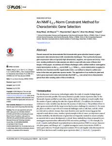


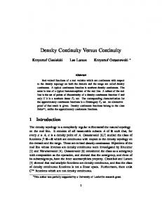

![[PDF] CCM Exam Secrets Study Guide: CCM Test ... - Google Sites](https://m.moam.info/img/260x300/pdf-ccm-exam-secrets-study-guide-ccm-test-google-s_647842e2097c4737708c9c00.jpg)

![[PDF] CCM Exam Secrets Study Guide: CCM Test ... - Google Sites](https://m.moam.info/img/260x300/pdf-ccm-exam-secrets-study-guide-ccm-test-google-s_647870f4097c474c228d237c.jpg)


