Cellular Automata as a Tool for Image Processing - Semantic Scholar

May 24, 2013

14:27

World Scientific Book - 9.75in x 6.5in

Chapter 1

Cellular Automata as a Tool for Image Processing

Paul L. Rosin and Xianfang Sun School of Computer Science & Informatics, Cardiff University Cardiff, CF24 3AA, UK E-mail: {Paul.Rosin,Xianfang.Sun}@cs.cf.ac.uk An overview is given on the use of cellular automata for image processing. We first consider the number of patterns that can exist in a neighbourhood, allowing for invariance to certain transformation. These patterns correspond to possible rules, and several schemes are described for automatically learning an appropriate rule set from training data. Two alternative schemes are given for coping with gray level (rather than binary) images without incurring a huge explosion in the number of possible rules. Finally, examples are provided of training various types of cellular automata with various rule identification schemes to perform several image processing tasks.

1.1

Introduction

Cellular automata (CA) consist of a regular grid of cells, each of which can be in only one of a finite number of possible states. The state of a cell is determined by the previous states of a surrounding neighbourhood of cells and is updated synchronously in discrete time steps. The identical rule contained in each cell is essentially a finite state machine, usually specified in the form of a rule table with an entry for every possible neighbourhood configuration of states. Cellular automata are discrete dynamical systems, and they have been found useful for simulating and studying phenomena such as ordering, turbulence, chaos, symmetry-breaking, etc, and have had wide application in modelling systems in areas such as physics, biology, and sociology. Over the last fifty years a variety of researchers (including well known names such as Stanislaw Ulam [Ulam (1962)] and John von Neumann [von Neumann (1966)], John Holland [Holland (1970)], Stephen Wolfram [Wolfram (1994)], and John Con1

book

May 24, 2013

14:27

2


P.L. Rosin & X. Sun

way [Gardner (1970)]) have investigated the properties of cellular automata. Particularly in the 1960’s and 1970’s considerable effort was expended in developing special purpose hardware (e.g. CLIP) alongside developing rules for the application of the CAs to image analysis tasks [Preston and Duff (1984)]. More recently there has been a resurgence in interest in the properties of CAs without focusing on massively parallel hardware implementations, i.e. they are simulated on standard serial computers. By the 1990’s CAs could be applied to perform a range of computer vision tasks, such as: • calculating distances to features [Rosenfeld and Pfaltz (1968)], • calculating properties of binary regions such as area, perimeter, convexity [Dyer and Rosenfeld (1981)], • performing medium level processing such as gap filling and template matching [de Saint Pierre and Milgram (1992)], • performing image enhancement operations such as noise filtering and sharpening [Hernandez and Herrmann (1996)], • performing simple object recognition [Karafyllidis et al. (1997)]. Cellular automata have a number of advantages over traditional methods of computations: • Although each cell generally only contains a few simple rules, the combination of a matrix of cells with their local interaction leads to more sophisticated emergent global behaviour. That is, although each cell has an extremely limited view of the system (just its immediate neighbours), localised information is propagated at each time step, enabling more global characteristics of the overall CA system. • This simplicity of implementation and complexity of behaviour means that CA can be better suited for modelling complex systems than traditional approaches. For example, for modelling shell patterns, CA were found to avoid the considerable numerical problems inherent with partial differential equation based models, and were also substantially faster to compute [Kusch and Markus (1996)]. • CA are both inherently parallel and computationally simple. This means that they can implemented very efficiently in hardware using just AND/OR gates and are ideally suited to VLSI realisation [Chaudhuri et al. (1997)]. • CA are extensible; rules can easily be added, removed or modified.

1.2

Relating the Number of Cell States to the Number of Rules

For a 3 × 3 neighbourhood with cells taking 256 possible intensities there are 2568 possible neighbourhood patterns (not considering the central cell’s value). However, for many image processing tasks this number can be reduced by considering symme-

book

May 24, 2013

14:27



ABA B B ABA

ABC D D CBA

book

3

ABA C C DED

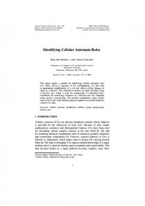
Fig. 1.1 Patterns of a 3 × 3 neighbourhood that remain invariant under ±90◦ rotation, 180◦ rotation, and mirror symmetry through a vertical line of reflection respectively.

tries, e.g. the same rule should apply even if the pattern is rotated. To determine the number of distinct patterns after removing equivalent symmetric versions the P´ olya-Burnside counting lemma [Roberts and Tesman (2005)] can be applied. If G is a set of permutations of a set A, then the number of equivalence classes is 1 X | Fix(g)| (1.1) N= |G| g∈G

where Fix(g) is the number of elements of A that are invariant under g. Figure 1.1 shows the patterns which are invariant under examples of the following transformations: ±90◦ rotation, 180◦ rotation, and mirror symmetry through a vertical line of reflection respectively. Thus, the number of distinct patterns N in terms of the number of possible intensities n is n8 + 2n2 + n4 + 4n5 (1.2) N= 8 where the terms in the numerator correspond to: the identity transformation (i.e. 0◦ rotation), two rotations (±90◦ ), a single rotation (180◦ ), and four rotations corresponding to mirror symmetry through horizontal, vertical, and diagonal lines of reflection. Given that even after eliminating symmetries the number of patterns still scales as O(n8 ), it can be seen that considering all n = 256 intensities leads to a prohibitive number of possible rules (N > 2×1018 ). Therefore, much of the previous application of cellular automata to image processing has been restricted to binary images. In this case, there are only 28 = 256 possible patterns or rules, which reduces to N = 51 rules after eliminating symmetries – see figure 1.2.

1.3

Threshold Decomposition

In order to extend binary image CA methods to apply to gray level images without incurring the combinatorial explosion in the number of rules, Rosin [Rosin (2006)] proposed using threshold decomposition, a technique used extensively in image processing for rank order filtering [Fitch et al. (1984)]. This involves decomposing the gray level image into the set of binary images obtained by thresholding at all possible gray levels.1 If a filter has the “stacking property” then it can be applied to 1 Since threshold decomposition using all intensity levels incurs a substantial computation cost, a subset of intensity levels can be used instead to produce a faster approximation.

May 24, 2013

14:27

4


P.L. Rosin & X. Sun

Fig. 1.2 The complete rule set for a 3 × 3 neighbourhood of binary values with a central black pixel contains 51 patterns after symmetries and reflections are eliminated. The black central pixel is flipped to white after application of the rule. The neighbourhood pattern of eight white and/or black (displayed as gray) pixels which must be matched is shown.

each binary image, and when the set of processed binary images are summed then the result is identical to applying the filter to the original intensity image. A set of CA rules do not in general satisfy the stacking property2 , nevertheless applying this methodology is still useful since it allows intensity images to be processed. There is no equivalence of the results using the binary CA to those of a full intensity CA, but experimental results showed that results were still good. In Rosin’s initial work the CA were trained to perform denoising on a single binary image and subsequently the learnt rule set was reapplied to a gray level image using threshold decomposition. This idea was subsequently developed [Rosin (2010)] to take the more computationally expensive approach of training the CA on gray level images. That is, a search is made for a set of rules that when applied to the elements of the threshold decomposed input image and reconstructed produces a gray level image that provides a good match to the gray level target image. This has the advantage that it directly optimises the desired error function unlike the first approach which does not use threshold decomposition in the training phase but only during the subsequent application phase.

1.4

A 3-State Representation

An alternative approach to reducing the number of cell states was proposed by Rosin [Rosin (2010)] to enable more efficient training and application of CA to intensity images. It is based on the texture unit texture spectrum (TUTS) method 2 Since CA can perform rank order filtering [Jagadish and Kailath (1989)] then it follows that at least some CA rules do possess the stacking property.

book

14:27



book

5

of texture analysis [Wang and He (1990)]. This involves using a pixel’s value as a threshold for its eight neighbours. That is, for a central pixel value vc its neighbours vi are thresholded as     0 if vi < vc ′ vi = 1 if vi = vc (1.3)    2 if v > v i

c

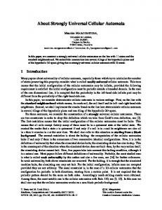
Each neighbourhood can then be represented by a code formed from the eight P8 ′ i 8 ternary values: i=1 vi 3 , and histograms of the 3 = 6561 different texture unit codes (the so called texture spectrum) make up the textural description of an image (or sub-image). This local thresholding approach can be used in the context of our CA to reduce the large number of neighbourhood patterns. The basic idea is to maintain at each cell the image intensity as its primary state, but during the rule matching phase to consider the ternary pattern of the neighbourhood determined relative to the central cell’s state. The CA rules are defined in terms of the 3 states rather than 256 states, and so from eqn. 1.2 we find that 954 patterns need be considered. local thresholding

ternary neighbourhood pattern

or e as e re as inc cre ity de ens int

ym a ru tch le? in g

pixel intensity

an

May 24, 2013

activated rule

Fig. 1.3 The CA is represented using both pixel intensities for cell states as well as ternary neighbourhood patterns. Transition rules involve changing a cell’s intensity sufficiently such that the ternary neighbourhood pattern changes.

The scheme is as follows, and is illustrated in figure 1.3. The rules are applied to all the matching cells in parallel at each time step. This involves 1/ first generating at each cell its ternary neighbourhood pattern by thresholding the neighbourhood according to eqn 1.3, 2/ at each cell check for any rule that matches its ternary neighbourhood pattern, 3/ if a rule matches then apply it to update the central cell. In a standard binary CA, application of a rule inverts the cell’s state. In the 3-state system despite using ternary rules it is the cell’s intensity that needs to be updated. This is done by modifying its value such that its ternary neighbourhood changes. The minimal modification in either direction is to either increase its intensity to its closest neighbourhood intensity value, or alternatively to decrease it to its closest neighbourhood value. Thus for each pattern there are two possible rules

May 24, 2013

14:27


6

P.L. Rosin & X. Sun

(i.e. increasing or decreasing types). Note that for each type of rule there are certain neighbourhood patterns that preclude the use of that rule type. That is, there are 51 of the 954 basic patterns without any neighbourhood pixel intensity greater than the central pixel, and the same number without a smaller value. Therefore, the total number of rules in this CA system is 2 × (954 − 51) = 1806. Two variations to the scheme are possible. The first allows all 1806 rules to be learnt independently. Thus, if the results of processing image I are f (I), there is no constraint that f (−I) = −f (I), which can be useful in some situations. The second variation enforces the constraint by treating the “increasing” and “decreasing” dec versions of a rule, RTinc Ui and RT Ui , as equivalent when applied to inverted neighdec bourhood intensities. That is, for a neighbourhood N , RTinc Ui (N ) ≡ RT Ui (−N ) and dec inc RT Ui (−N ) ≡ RT Ui (N ), and so there are only 903 rules to be learnt. One of the features of the TUTS (and LBP) schemes is that they provide a textural description that is invariant to a wide range of gray level transformations. Thus, for the 3-state CA this means that f (T (I)) = T (f (I)) where T is a monotonic, non-linear mapping that is information preserving in the sense that separate intensities are not collapsed into single values. In some situations this could be beneficial, but in others a lot of important information is lost by discarding quantitative information, and so the 3-state CA is not suited to solve certain quantitative tasks, e.g. computing edge magnitudes.

1.5

Training Strategies

Most of the literature on cellular automata studies the effect of applying manually specified transition rules. However, this is not a convenient way in which to build an image processing system, and a more automated approach is required. Ideally, it should be possible to automatically learn the rules given 1/ a set of training images, 2/ a set of corresponding target (i.e. ideal) output images, and 3/ an objective function for evaluating the quality of the actual images produced by the CA, i.e. the error between the target output and the CA output. However, the inverse problem of determining appropriate rules to produce a desired effect is hard [Ganguly et al. (2003)]. In general an optimal selection of rules cannot be guaranteed without an exhaustive enumeration of all combinations [Cover and Campenhout (1977)], and this is clearly generally not feasible. We shall describe three more practical approaches for learning appropriate rule sets from training data. 1.5.1

Genetic Algorithms

The most common approach in the literature is to use evolutionary algorithms, and in particular genetic algorithms (GAs). Most of this work is applied to a single, somewhat artificial, example which is a version of the density classification problem on a 1D grid. Given a binary input pattern, the task is to decide if there are a

book

May 24, 2013

14:27



book

7

majority of 1s or not, i.e, a single binary outcome. For CAs with rules restricted to small neighbourhoods this is a non-trivial task since the 1s can be distributed through the grid, and so it requires global coordination of distant cells that cannot communicate directly. Early work by Mitchell et al. [Mitchell et al. (1994)] encountered several difficulties with the GA learning: 1/ breaking of symmetries in early generations for short-term gains, and 2/ the training data became too easy for the CAs in later generations of the GA. Juillé and Pollack [Juillé and Pollack (1998)] tackled the latter problem using GAs with co-evolution. To encourage better learning the training set was not fixed during evolution, but gradually increased in difficulty. Thus, once initial solutions for simple versions of the problem were learnt, they would be extended and improved by evolving the data to become more challenging. Instead of GAs Andre et al. [Andre et al. (1996)] used a standard genetic programming framework. Since this was computationally expensive it was run in parallel on 64 PCs. Extending the density classification task to 2D grids, Jiménez Morales et al. [Morales et al. (2001)] again applied standard GA to learn rules. Applying GAs remains a dominant theme in research into learning CA rules [Bull and Adamatzky (2007); Terrazas et al. (2007)], although progress is limited. There are still papers attempting to solve the trivial task of binary image boundary detection using genetic algorithms and CA [Batouche et al. (2006); Slatnia et al. (2007)]. Another example at the same level attempts (with limited success) to generate simple shapes such as a square, circle, etc., again using genetic algorithms [Chavoya and Duthen (2006)]. Craiu and Lee [Craiu and Lee (2006)] use a minimum description length criterion to automatically learn both neighbourhood size and rules for stochastic CA to perform the task of synthesising binary patterns. However, the system exhaustively considers first all neighbourhood sizes and then all rule parameters, and so they could only demonstrate results on very small CA examples. Greedy Selection

1.5.2

In comparison to such evolutionary methods, deterministic feature selection methods are extensively used for building classifier systems. In particular, we describe a popular approach called the sequential floating forward search (SFFS) [Pudil et al. (1994)] which was found to perform best compared to fourteen other feature selection algorithms (including a genetic algorithm) [Jain and Zongker (1997)]. SFFS was first used for training CA for image processing tasks by Rosin [Rosin (2006)]. The advantages of deterministic feature selection methods over evolutionary methods are that • • • •

they tend to be extremely simple to implement their runtime is significantly less the quality of their results is as good or better being deterministic rather than randomised means that the results are re-

May 24, 2013

14:27

8


P.L. Rosin & X. Sun

peatable (which is particularly helpful for other researchers attempting to duplicate published results) • they do not require the many parameters necessary for genetic algorithms. The SFFS algorithm can be described as follows. Let Ri denote the rule set at iteration i and its score be J (Ri ). In our case, J (Ri ) is computed by applying the CA with the rule set Ri to the input image, and returning the error computed by one of the objective functions described in the next section. The initial rule set R0 is empty. At each iteration i all rules are considered for addition to the rule set Ri−1 . Only the rule giving the best score is retained, to make Ri . This process is repeated until no improvements in score are gained by adding rules (an alternative termination rule is when a known desired number of rules has been found). This describes the sequential forward search, which is extended to the sequential floating forward search by interleaving between each iteration the following test. One at a time, each rule in Ri is removed to find the rule whose removal provides the candidate rule set R′i−1 with the best score. If this score is better than J (Ri−1 ) then Ri is discarded, Ri−1 is replaced by R′i−1 , and the process continues with the addition of the i’th rule. Otherwise, R′i−1 is discarded, and the process continues with the addition of the (i + 1)’th rule to Ri . 1.5.3

Identification Algorithms

Genetic algorithms or greedy selection methods can be used to learn CA rules from training data pairs effectively, but the learning procedure is very time-consuming. If only input/output data pairs (representing start/end CA states) are available, and multiple steps of CA evolution from the start to the end states are required, the above introduced CA rule learning methods are still the state-of-the-art ones. However, if the start and the end together with their intermediate CA states are available, or only one step is needed to evolve from the start to the end states, fast CA learning methods exist. Recent development in CA rule extraction for the cases with intermediate CA states involves parameter estimation methods from the field of system identification [Adamatzky (1994); Billings and Yang (2003a); Billings and Mei (2005); Zhao and Billings (2007); Sun et al. (2011); Billings and Yang (2003b)]. The basic idea underlying identification algorithms for CA rule learning is as follows. CA rules are modelled as a linear-in-parameter model, and the model parameters are estimated based on some error minimisation criterion using the start, the intermediate, and the end states. The model together with the estimated parameter values is then used to retrieve the CA rules. Not only are such approaches fast, but are also effective for larger neighbourhood sizes than are practical for the previous methods. The current fastest CA identification algorithm was developed by Sun et al. [Sun et al. (2011)], and the following is a brief description of the algorithm. Let xi (t) be the state value of cell ci at evolution step t, and xli (t)(l = 1, . . . , m)

book

May 24, 2013

14:27



book

9

be the state values of the cells in ci ’s neighbourhood at step t. The state value of ci at step t + 1 is then given by xi (t + 1) =

m 2X −1

θj Qji (t) + ǫi (t),

(1.4)

j=0

where Qji (t) is the value of j th neighbourhood pattern defined by Qji (t)

=

m Y

blj (xli (t)),

(1.5)

l=1

and blj is defined as the coefficient of 2l−1 in j when j is written as a binary number. θj is either 0 or 1, and θj = 0 represents the CA rule that when the neighbourhood state combination is pattern Qji (t), xi (t + 1) takes value 0, while θj = 1 means that xi (t + 1) takes value 1. ǫi (t) is a noise term, which is to be minimised in the estimation of the parameters. Note that here m is the neighbourhood size and the number of neighbourhood patterns is 2m . Although in the context of image processing in this chapter, the neighbourhood size is 9 (including the central cell), and the number of patterns is reduced from 29 = 512 to 51 × 2 = 102 when considering rotation and mirror symmetry, we used all the 512 original patterns in Eqn. 1.4 in the identification experiments in this chapter. However, the readers can easily generalise Eqn. 1.4 to the case of 102 patterns. When noise variance is used as the minimisation criterion, the parameter estimation problem is solved by 2  m 2X −1 C T X X 1 j xi (t + 1) − θj Qi (t) , (1.6) {θˆj } = arg min T C t=1 i=1 j=0 where T is the number of evolution steps, and C the number of cells. Considering that xi (t + 1), θj and Qji (t) always take values 0 or 1, the solution of Eqn. 1.6 is reduced to ( 1, if rj > 0, j θˆ = (1.7) 0, if rj ≤ 0, where rj =

C T 1 XX (xi (t + 1) − x ¯i (t + 1)) Qji (t), T C t=1 i=1

(1.8)

and x ¯i (t + 1) denotes the logical NOT of xi (t + 1). Sun et al. [Sun et al. (2011)] also discussed automatic selection of the CA neighbourhood size and gave an incremental neighbourhood algorithm that uses the Bayesian information criterion. The readers are referred to the original paper [Sun et al. (2011)] for details.

May 24, 2013

14:27


10

1.5.4

P.L. Rosin & X. Sun

Objective Functions

Whichever optimisation method is used, an objective function is required, and its quality obviously has a crucial effect on the final results. For binary images the simplest objective function is the Hamming distance, or for images with more intensity values then the root mean square (RMS) error between the input and target image is a straightforward measure. However, it is well known that RMS (and related) values have limitations. In particular, given that they do not involve inter-pixel relationships they often do not capture perceptual similarity. One possible improvement which incorporates spatial information into the comparison of binary images A and B is to use the Hausdorff distance H(A, B) = max min ||a − b||. a∈A b∈B

For grey level images a well known image similarity measure is the Structural Similarity index (SSIM) [Wang et al. (2004)]which takes luminance, contrast and structure into account: SSIM (A, B) =

(2µA µB + C1 )(2σAB + C2 ) 2 + σ2 + C ) . + µ2B + C1 )(σA 2 B

(µ2A

where the constants are set to C1 = (0.01×255)2 and C2 = (0.03×255)2 . The SSIM index is then applied locally using an 11×11 circular-symmetric Gaussian weighting function, and the mean over the image is used as the final similarity measure. 1.6 1.6.1

Applications of Cellular Automata to Image Processing Binary Image Denoising

The effectiveness of the CA is first demonstrated on binary image denoising. To demonstrate the differences between the three training strategies described in section 1.5, each was applied to learn the rule sets for the five input conditions (corresponding to three types/levels of noise). The GA used in our study was a simple steady state GA [Syswerda (1989); Mumford-Valenzuela et al. (2003)]. During crossover, the first parent is selected deterministically in sequence, but the second parent is selected uniformly, at random. If new offspring duplicate existing values for the objective function, then they automatically “die”. The GA was run for a fixed number of generations (100) and the population size was set to 100. For each image, the GA was run ten times with different initialisations of the random number generator. For the identification algorithm, we considered two cases: one uses the 3 × 3 neighbourhood with size m = 9 which includes neighbours {c(i, j) : |i−i0 |, |j −j0 | ≤ 1} corresponding to the central cell c(i0 , j0 ), and the other uses the neighbourhood with size m = 13 which includes neighbours {c(i, j) : |i − i0 | + |j − j0 | ≤ 2}.

book

May 24, 2013

14:27


book

11

Cellular Automata as a Tool for Image Processing Table 1.1 RMS errors of filtered versions of the binary test image corrupted by salt and pepper noise with probabilities p = 0.01, 0.1, 0.3; black squares containing a white central pixel; and black ‘T’s and white bars. For the GA the mean RMS over the ten runs is given with the standard deviation in brackets. For the median filter the RMS is given for the number of iterations (which is indicated in brackets) that gave the best results on the test image. noise original CA median type image GA SFFS Identification filter m=9 m = 13 S & P, p = 0.01

17.9

14.6 (0.3)

14.1

14.1

12.7

42.5 (1)

S & P, p = 0.1

57.0

41.2 (0.4)

32.4

32.3

30.6

45.0 (1)

S & P, p = 0.3

99.0

49.5 (1.0)

47.6

49.2

49.0

53.3 (2)

B & W square

55.7

48.9 (5.6)

32.0

32.0

25.8

55.7 (0)

‘T’s and bars

64.1

65.5 (1.9)

48.2

54.3

44.1

64.1 (0)

Two large binary images (1536 × 1024 pixels) were constructed, one each for training and testing, and consisted of a composite of several 256 × 256 subimages obtained by thresholding standard images. Different types and levels of noise were added, and a set of rules learnt for each. Salt and pepper noise was added with probabilities p = 0.01, 0.1, 0.3. The next two types of noise are non-standard, and were included to demonstrate how the CA can learn good rules as long as it has good training data. Black squares (3×3) containing a single white central pixel were added; the final noise type consisted of added black ‘T’s and white bars. Examples of these noise types are shown in figure 1.4. In all instances the rules were run for up to 100 iterations. For comparison, results of filtering are providing using a 3 × 3 median filter with the optimal number of iterations determined for the test image, giving the median a favourable bias. As table 1.1 shows, for small amounts of noise the median filter degrades the image rather than improves it. Likewise, it is unable to cope with the unusual noise types (squares and ‘T’s/bars). In comparison, the CA (when trained using SFFS or the identification algorithm) consistently succeeds in denoising the images, and also improves on the median filter’s results in all cases. The results are demonstrated visually on a small image window in figure 1.4. For the lowest level of salt and pepper noise (p = 0.01) the CA learns to use a . As the noise level increases the number single rule to remove isolated pixels: and the rules for of rules required increases. For p = 0.1 the rules are: p = 0.3 are: . For noise consisting of the black square with . white central pixel the following rules were learnt: Unlike the salt and pepper noise in which the rules also applied in their inverted versions (i.e. swapping the roles of black and white), the learnt rules for square were (automatically) determined only to operate when the central pixel was black. For the black ‘T’s and white bars noise the rules learnt for patterns with a black and one further rule to be applied for white central pixel were:

May 24, 2013

14:27


12

book

P.L. Rosin & X. Sun

(A)

(B)

(C)

(D) (a)

(b)

(c)

(d)

(e)

Fig. 1.4 Examples of binary image denoising. Rows show (A) the input images, and the results after denoising using (B) CA trained by SFFS , (C) CA generated by identification algorithm (D) median filtering. Columns (a)–(e) show different noise conditions: salt and pepper p = 0.01, salt and pepper p = 0.1, salt and pepper p = 0.3, added black square with white central pixel, added black ‘T’s and white bars. One iteration of the median filter was applied except for (c) for which two iterations were applied.

central pixels: . Table 1.1 shows that the GA was not competitive with the other training meth-

May 24, 2013

14:27


book

13

Cellular Automata as a Tool for Image Processing Table 1.2 Timings (in seconds) for learning the rules for the binary image filtering tasks. noise CA type GA SFFS Identification S & P, p = 0.01

1427

46

S & P, p = 0.1

8717

290

8 8

S & P, p = 0.3

14230

843

8

B & W square

2776

2493

8

‘T’s and bars

25030

4483

8

ods, generating much worse results. Furthermore, it can be seen from table 1.2 that its runtime is much greater. From these experiments it is evident that identification algorithm generally performed the best out of the three training methods, both in terms of accuracy and computational efficiency. 1.6.2

Gray Level Denoising Table 1.3 RMS errors of filtered versions of the gray level test image corrupted by Gaussian noise, single pixel salt and pepper noise, salt and pepper noise affecting 3 × 3 pixel blocks, and randomly recoloured stripes. noise original CA shock AM type TD 3-state filter Gaussian, σ = 25

23.7

13.9

13.9

16.1

18.9

S & P, p = 0.6

113.5

25.0

20.9

58.5

18.8

3 × 3 S & P, p = 0.01

43.1

14.7

11.8

37.9

12.1

stripe, p = 0.8

83.3

54.0

35.4

62.7

65.1

Using either of the two techniques described in section 1.5 the CA for binary image denoising can be extended to perform gray level denoising. Results of experiments are shown here along with a comparison made with the complex shock filter [Gilboa et al. (2004)]3 and the adaptive median (AM) filter [Hwang and Haddad (1995)]. The CA was trained and tested on the grey level versions of the 1536 × 1024 image mosaics used for the binary image denoising experiments in section 1.6.1. The SFFS training strategy and the RMS objective function were used, and the number of rule iterations was set to 100. Various types of noise were added: salt and pepper, and 3 × 3 blocks of salt and pepper. As with the binary image denoising a non-standard noise was included to show the capabilities of learning noise specific rules. This structured noise was created by randomly replacing (with probability p) each row or column in the image with a random intensity (constant along the stripe). Thus the probability of 3 Gilboa’s code for his complex shock filter was used with its default parameters: number of ˜ = 0.2 and a = 2. iterations = 30, |λ| = 0.1, λ

May 24, 2013

14:27


14

book

P.L. Rosin & X. Sun

(A)

(B)

(C)

(D) (a)

(b)

(c)

(d)

(a)

(b)

(c)

(d)

(E)

Fig. 1.5 Examples of grey level image denoising. Rows show (A) the input images, and the results after denoising using (B) CA with threshold decomposition, (C) 3-state CA, (D) complex shock filter, and (E) the adaptive median filter. Columns (a)–(d) show different noise conditions: Gaussian σ = 25; salt and pepper p = 0.6, single pixel; salt and pepper, 3 × 3 block, p = 0.01; stripe p = 0.8.

May 24, 2013

14:27


book


15

2 corrupting a pixel is p − p2 . The RMS errors resulting from denoising are listed in table 1.3, and examples of the results from applying the various methods are displayed in figure 1.5. The CA generally performs well, and the 3-state CA gives lower errors than the threshold decomposition CA. For the case of Gaussian noise it outperforms the shock filter and adaptive median, although there certainly exist other denoising methods that work better on this type of noise (although not so well on other noise types), e.g. the hidden Markov trees (HMT) applied to wavelet coefficients [Romberg et al. (2001)] that were previously compared against CA for denoising in [Rosin (2010)]. The adaptive median is well suited to salt and pepper noise (i.e. where the noise is at the extreme ends of the intensity range) but does not do so well for the stripe noise which consists of random intensities. 1.6.3

Edge Detection

(a) Fig. 1.6

(b)

Training data for edge detection task. (a) input image, (b) target image.

We now demonstrate the training and application of CA to edge detection. To create a good set of training data a 750 × 750 image mosaic was created using subimages from the University of South Florida data set which contains images along with manually generated ground truth edges – see figure 1.6. Since there is likely to be some positional error in the ground truth edges (which are one pixel wide) the target edge map was dilated twice, with the new edges set each time to an increasingly lower intensity. This process is similar to blurring the edge map whilst avoiding creating local intensity maxima at junctions. Since the 3-state CA representation discards most of the intensity magnitude

May 24, 2013

14:27


16

book

P.L. Rosin & X. Sun

(a)

(b)

(c)

(d)

(e)

Fig. 1.7 Edge detection using the threshold decomposition CA. (a) input image, (b) results from CA, (c) noisy input image, (d) results of filtering figure 1.7c using a CA trained on corrupted version of figure 1.6a, (e) results of filtering figure 1.7c using the Sobel edge detector.

information there is insufficient information to compute edge magnitudes, and therefore this approach is not appropriate for performing edge detection. However, the threshold decomposition method works well as demonstrated in figure 1.7b which used the SFFS training strategy and RMS objective function. In fact, the rule set is exceedingly simple, consisting of a single rule, specifying that any white pixel in a 3 × 3 homogeneous (i.e. all white) neighbourhood is flipped. For each of the binary images that the input is decomposed into, this causes all white pixels to be replaced by black except for pixels adjacent to black pixels in the input image. Thus, a black image is formed containing a one pixel wide white strip along the original black/white transitions, which when summed at the reconstruction stage of the threshold decomposition produces the edge magnitudes. An advantage of the CA methodology is that rules can be combined to perform multiple tasks. This is demonstrated by adding noise to the training image in figure 1.6a, specifically 3 × 3 blocks of white pixels. Retraining the CA produces rules that simultaneously perform denoising whilst detecting edges. The results of applying the new rules to the noisy image in figure 1.7c are shown in figure 1.7d. In comparison to the Sobel edge detector the CA is much more successful in being able to robustly detect the edges, the results being only minimally affected by the salt and pepper noise. 1.7

Conclusions and Discussion

As demonstrated in this chapter, it is possible to automatically learn rules for cellular automata that can effectively perform image processing tasks. Examples have been given here for image denoising and edge detection, and further examples (convex hull, connected set morphology, ridge detection) were shown in [Rosin (2006, 2010)]. A benefit of the CA approach is that it is flexible, and can easily be applied to a variety of tasks; the same architecture can be used, and the CA just needs retraining with new data.

May 24, 2013

14:27



book

17

It is crucial to have good methods for automatically learning the CA rules, and we have described those that are currently popular in the literature. Although genetic algorithms are the most commonly used they were shown to be the worst choice, being both slow and providing relatively poor solutions. In comparison, the greedy algorithms (such as sequential floating forward search) were faster and gave better results. Under certain circumstances, the system identification type algorithm was able to perform very well, with substantially reduced computation time. However, it assumes the availability of training data containing the desired outputs at intermediate iterations of the CA, which are unlikely to be available for the image processing tasks. Therefore, the system identification algorithm is most effective for image processing when the number of iterations required for the task is small (ideally one). Another important factor is the objective function used for optimisation by the rule selection algorithms. Although several possibilities were considered, it has not been shown that the more sophisticated functions that incorporate spatial information provided significant benefits over the simpler functions such as root mean square error [Rosin (2006, 2010)]. There are several directions for future research: • Although both the threshold decomposition and the 3-state approaches to extending the binary state cellular automata to operate on gray level images were effective, it would be worthwhile investigating alternatives that are better able to capture the gray level information while maintaining reasonable computational complexity. • The system identification algorithm is very promising, and if it could be extended to cope with missing input/output data pairs this would greatly increase its usefulness. • Most of the results described here and in the literature used small neighbourhoods (e.g. 3 × 3). It would be of interest to experiment with larger neighbourhoods which definitely provide the possibility of better results. However, this would also increase the cost in terms of storage requirements, computation time, and would need larger amounts of training data for effective rule identification.

May 24, 2013

14:27


Bibliography

Adamatzky, A. (1994). Identification of Cellular Automata (Taylor & Francis, London, UK), ISBN 0-7484-0172-5. Andre, D., III, F. B. and Koza, J. (1996). Discovery by genetic programming of a cellular automata rule that is better than any known rule for the majority classification problem, in Proc. 1st Conf. on Genetic Programming (MIT Press), pp. 3–11. Batouche, M., Meshoul, S. and Abbassene, A. (2006). On solving edge detection by emergence, in Int. Conf. on Industrial, Engineering and Other Apps. of Applied Intelligent Systems, Vol. LNAI 4031, pp. 800–808. Billings, S. and Yang, Y. (2003a). Identification of probabilistic cellular automata, IEEE Transactions on Systems Man and Cybernetics, Part B: Cybernetics 33, 2, pp. 225– 236. Billings, S. and Yang, Y. (2003b). Identification of the neighborhood and CA rules from spatio-temporal CA patterns, IEEE Trans. on Systems, Man and Cybernetics, Part B 33, 2, pp. 332–339. Billings, S. A. and Mei, S. S. (2005). A new fast cellular automata orthogonal least-squares identification method, International Journal of Systems Science 36, 8, pp. 491–499. Bull, L. and Adamatzky, A. (2007). A learning classifier system approach to the identification of cellular automata, J. Cellular Automata 2, 1, pp. 21–38. Chaudhuri, P., Chowdhury, D., Nandi, S. and Chattopadhyay, S. (1997). Theory and Applications: Additive Cellular Automata (IEEE Press). Chavoya, A. and Duthen, Y. (2006). Using a genetic algorithm to evolve cellular automata for 2D/3D computational development, in Genetic and Evolutionary Comp. Conf., pp. 231–232. Cover, T. and Campenhout, J. V. (1977). On the possible orderings in the measurement selection problem, IEEE Trans. on Systems, Man and Cybernetics 7, 9, pp. 657–661. Craiu, R. and Lee, T. (2006). Pattern generation using likelihood inference for cellular automata, IEEE Trans. on Image Processing 15, 7, pp. 1718–1727. de Saint Pierre, T. and Milgram, M. (1992). New and efficient cellular algorithms for image processing, CVGIP: Image Understanding 55, 3, pp. 261–274. Dyer, C. and Rosenfeld, A. (1981). Parallel image processing by memory-augmented cellular automata, IEEE Transactions on Pattern Analysis and Machine Intelligence 3, 1, pp. 29–41. Fitch, J., Coyle, E. and Gallagher, N. (1984). Median filtering by threshold decomposition, Acoustics, Speech and Signal Processing, IEEE Transactions on 32, 6, pp. 1183– 1188. Ganguly, N., Sikdar, B., Deutsch, A., Canright, G. and Chaudhuri, P. (2003). A survey on

19

book

May 24, 2013

14:27

20


P.L. Rosin & X. Sun

cellular automata, Tech. Rep. 9, Centre for High Performance Computing, Dresden University of Technology. Gardner, M. (1970). The fantastic combinations of John Conway’s new solitaire game “life”, Scientific American , pp. 120–123. Gilboa, G., Sochen, N. and Zeevi, Y. (2004). Image enhancement and denoising by complex diffusion processes, IEEE Trans. on Pattern Analysis and Machine Intelligence 26, 8, pp. 1020–1036. Hernandez, G. and Herrmann, H. (1996). Cellular automata for elementary image enhancement, Graphical Models and Image Processing 58, 1, pp. 82–89. Holland, J. (1970). Logical theory of adaptive systems, in A. Burks (ed.), Essays in Cellular Automata (University of Illinois Press). Hwang, H. and Haddad, R. (1995). Adaptive median filters: new algorithms and results, IEEE Trans. on Image Processing 4, 4, pp. 499–502. Jagadish, H. and Kailath, T. (1989). Primitive cellular automata, threshold decomposition, and ranked order operations, IEEE Trans. Comput. 38, pp. 148–149. Jain, A. and Zongker, D. (1997). Feature-selection: Evaluation, application, and small sample performance, IEEE Trans. on Pattern Analysis and Machine Intelligence 19, 2, pp. 153–158. Juillé, H. and Pollack, J. (1998). Coevolving the ideal trainer: Application to the discovery of cellular automata rules, in Proc. 3rd Conf. on Genetic Programming (Morgan Kaufmann), pp. 519–527. Karafyllidis, I., Ioannidis, A., Thanailakis, A. and Tsalides, P. (1997). Geometrical shape recognition using a cellular automaton architecture and its VLSI implementation, Real-Time Imaging 3, pp. 243–254. Kusch, I. and Markus, M. (1996). Mollusc shell pigmentation: cellular automaton simulations and evidence for undecidability, J. Theor. Biol. 178, pp. 333–340. Mitchell, M., Hraber, P. and Crutchfield, J. (1994). Evolving cellular automata to perform computation: Mechanisms and impedients, Physica D 75, pp. 361–391. Morales, F. J., Crutchfield, J. and Mitchell, M. (2001). Evolving two-dimensional cellular automata to perform density classification: a report on work in progress, Parallel Computing 27, pp. 571–585. Mumford-Valenzuela, C., Vick, J. and Pearl, Y. (2003). Heuristics for large strip packing problems with guillotine patterns: An empirical study, in D. Du and P. Pardalos (eds.), Metaheuristics: Computer Decision-Making (Kluwer Academic Press). Preston, K. and Duff, M. (1984). Modern Cellular Automata-Theory and Applications (Plenum Press). Pudil, P., Novovicova, J. and Kittler, J. (1994). Floating search methods in featureselection, Pattern Recognition Letters 15, 11, pp. 1119–1125. Roberts, F. and Tesman, B. (2005). Applied Combinatorics (Pearson/Prentice-Hall). Romberg, J., Choi, H. and Baraniuk, R. (2001). Bayesian tree-structured image modeling using wavelet domain hidden markov models, IEEE Trans. on Image Processing 10, 7, pp. 1056–1068. Rosenfeld, A. and Pfaltz, J. (1968). Digital distance functions on digital pictures, Pattern Recognition 1, 1, pp. 33–61. Rosin, P. (2006). Training cellular automata for image processing, IEEE Trans. on Image Processing 15, 7, pp. 2076–2087. Rosin, P. (2010). Image processing using 3-state cellular automata, Computer Vision and Image Understanding 114, 7, pp. 790–802. Slatnia, S., Batouche, M. and Melkemi, K. (2007). Evolutionary cellular automata basedapproach for edge detection, in Int. Workshop on Fuzzy Logic and Applications, Vol.

book

May 24, 2013

14:27


Bibliography

book

21

LNAI 4578, pp. 404–411. Sun, X., Rosin, P. and Martin, R. (2011). Fast rule identification and neighborhood selection for cellular automata, IEEE Transactions on Systems Man and Cybernetics, Part B: Cybernetics 41, 3, pp. 749–760. Syswerda, G. (1989). Uniform crossover in genetic algorithms, in Proc. Third Int. Conf. on Genetic Algorithms (Lawrence Erlbaum Associates), pp. 2–9. Terrazas, G., Siepmann, P., Kendall, G. and Krasnogor, N. (2007). An evolutionary methodology for the automated design of cellular automaton-based complex systems, J. Cellular Automata 2, 1, pp. 77–102. Ulam, S. (1962). On some mathematical problems connected with patterns of growth of figures, in Proc. Symp. Appl. Math., Vol. 14, pp. 215–224. von Neumann, J. (1966). Theory of Self-Reproducing Automata (University of Illinois Press). Wang, L. and He, D. (1990). Texture classification using texture spectrum, Pattern Recognition 23, pp. 905–910. Wang, Z., Bovik, A., Sheikh, H. and Simoncelli, E. (2004). Image quality assessment: from error visibility to structural similarity, IEEE Trans. on Image Processing 13, 4, pp. 600–612. Wolfram, S. (1994). Cellular Automata and Complexity Collected Papers (AddisonWesley). Zhao, Y. and Billings, S. (2007). The identification of cellular automata, Journal of Cellular Automata 2, 1, pp. 47–65.