Chaotic Multiobjective Evolutionary Algorithm Based on

Hindawi Publishing Corporation Mathematical Problems in Engineering Volume 2014, Article ID 640764, 25 pages http://dx.doi.org/10.1155/2014/640764

Research Article Chaotic Multiobjective Evolutionary Algorithm Based on Decomposition for Test Task Scheduling Problem Hui Lu, Lijuan Yin, Xiaoteng Wang, Mengmeng Zhang, and Kefei Mao School of Electronic and Information Engineering, Beihang University, Beijing 100191, China Correspondence should be addressed to Hui Lu; [email protected] Received 13 March 2014; Revised 20 June 2014; Accepted 20 June 2014; Published 15 July 2014 Academic Editor: Jyh-Hong Chou Copyright © 2014 Hui Lu et al. This is an open access article distributed under the Creative Commons Attribution License, which permits unrestricted use, distribution, and reproduction in any medium, provided the original work is properly cited. Test task scheduling problem (TTSP) is a complex optimization problem and has many local optima. In this paper, a hybrid chaotic multiobjective evolutionary algorithm based on decomposition (CMOEA/D) is presented to avoid becoming trapped in local optima and to obtain high quality solutions. First, we propose an improving integrated encoding scheme (IES) to increase the efficiency. Then ten chaotic maps are applied into the multiobjective evolutionary algorithm based on decomposition (MOEA/D) in three phases, that is, initial population and crossover and mutation operators. To identify a good approach for hybrid MOEA/D and chaos and indicate the effectiveness of the improving IES several experiments are performed. The Pareto front and the statistical results demonstrate that different chaotic maps in different phases have different effects for solving the TTSP especially the circle map and ICMIC map. The similarity degree of distribution between chaotic maps and the problem is a very essential factor for the application of chaotic maps. In addition, the experiments of comparisons of CMOEA/D and variable neighborhood MOEA/D (VNM) indicate that our algorithm has the best performance in solving the TTSP.

1. Introduction Test task scheduling problem (TTSP) is an essential part of the automatic test system for improving throughput, reducing time, and optimizing resource allocation. Similar to other scheduling problems, the TTSP is one kind of combination optimization problems. It is illustrated to be an NP-hard problem through the analysis of the nature of the problem carried out by many researchers [1–3]. In addition, through the fitness distance analysis [4], we know that the TTSP has many local optima. The algorithm that has strong space searching ability is needed to solve the TTSP. Recently, many intelligent methods are used for solving the TTSP and other similar scheduling problems based on the problems’ character. All these kinds of researches focus on improving the searching ability of the algorithm and obtaining optimal or near-optimal solutions for the scheduling problem. There are two basic strategies. One is to propose an improvement algorithm based on the original algorithm, such as variable neighborhood multiobjective optimization algorithm based on decomposition (VNM) for the multiobjective test task scheduling problem [5]. Another

is to adopt a hybrid algorithm using two different kinds of algorithms. For example, Lu et al. proposed a hybrid particle swarm optimization and taboo search strategies for the single objective TTSP [6]. Recently, the hybrid method becomes a mainstream. Different from the hybrid method using different kinds of algorithms, using chaos in the evolutionary process represents its advantages in improving the searching ability. Lu et al. proposed a chaotic nondominated sorting genetic algorithm for the multiobjective test task scheduling problem and validated the best performance in convergence and diversity through the experiment and analysis [1]. Donald et al. utilized the chaos-induced discrete self-organizing migrating algorithm to solve the lot-streaming flow shop scheduling problem with setup time [7]. Gavrilova and Ahmadian studied an on-demand chaotic neural network for the broadcast scheduling problem and found an optimal time division multiple access (TDMA) frame [8]. Jiang et al. proposed a chaos-based fuzzy regression approach to model customer satisfaction for product design and used a chaotic optimization algorithm to generate the polynomial structures

2 of customer satisfaction models [9]. Sun et al. studied a novel hysteretic noisy chaotic neural network for broadcast scheduling problems in packet radio networks and exhibited a stochastic chaotic simulated annealing algorithm [10]. The phenomenon that occurred in these researches illustrated that the evolutionary algorithm embedded with chaos is an effective and efficient approach for improving the searching ability of the algorithm. However, all these researches have the same defect. The authors only used one or several chaotic maps embedded in algorithms to solve practical problems. However, there is no detailed discussion and analysis. For the TTSP, notice that the previous studies mostly aim at a single objective and only few papers focus on the multiobjective problem [1, 5]. Through the analysis of our previous related work for the multiobjective TTSP, we know the multiobjective evolutionary algorithm based on decomposition (MOEA/D) exhibited the best performance in solving the TTSP [5] in the aspect of convergence and diversity. Therefore, using chaotic maps in MOEA/D can further enhance the quality of the solution for the TTSP. In this paper, we propose a chaotic multiobjective evolutionary algorithm based on decomposition (CMOEA/D) for the TTSP. Ten chaotic maps are embedded in three different phases in the evolutionary process. The aim is to give guidance for the choice of chaotic maps and phases based on the framework of MOEA/D for the TTSP. First, the chromosome-encoding scheme is very important for the problem description and the operation in the evolutionary process. For the TTSP, there are different kinds of encoding strategies, like task sequencing list (TSL) (or the operations list coding (OLC)), matrix-encoding, and integrated encoding scheme (IES). TSL and matrix-encoding are not acceptable if a task can be tested on more than one set of instruments. IES can overcome this problem, but it cannot realize the selection operation under equal probability. Therefore, in this paper, the improved IES is proposed by changing the schemes selection method of every test task. As a result, the equal probability is realized. Then, ten chaotic maps are embedded in MOEA/D independently in three phases. The ten chaotic maps are baker’s map, cat map, circle map, cubic map, Gauss map, ICMIC map, logistic map, sinusoidal map, tent map, and Zaslavskii map. Three phases are initial population, crossover operator, and mutation operator. Four benchmarks of the TTSP are used to evaluate the performance of the proposed algorithm. They are 6 × 8, 20 × 8, 30 × 12, and 40 × 12. We use 𝑛 × 𝑚 to represent the benchmark. Here, 𝑛 is the number of tasks and 𝑚 is the number of instruments. The performance metrics hypervolume (HV) and 𝐶 [11] are used to evaluate the role of chaotic maps on MOEA/D. Therefore, we can find which kind of chaotic map embedded algorithm is the best one for solving the TTSP. From the results of experiments, it can be seen that the chaotic map embedded MOEA/D has good performance to solve the TTSP for both small and large scale problems. Different kinds of chaotic maps have different performances in different phases of MOEA/D, but ICMIC map and circle map in initial population, crossover operator, and mutation operator have the best performance. The experiments for

Mathematical Problems in Engineering comparisons of CMOEA/D and VNM show that our algorithm performs better than the VNM in solving the TTSP. The evidence, the chaotic map is an effective and efficient method for solving the problem with local optima, is validated. The similarity degree of distribution between chaotic maps and the problem is a very essential factor for the application of chaotic maps. The rest of the paper is organized as follows. Section 2 gives a summary of related work on applying chaos to improve evolutionary algorithms. Section 3 concludes the mathematical model proposed by us in previous work for the integrity. In Section 4, ten chaotic maps including both one-dimensional maps and two-dimensional maps are introduced. In Section 5, the proposed CMOEA/D is described in detail for solving the TTSP. The detail of the encoding scheme and the phases in which chaos can be embedded in evolutionary algorithms are introduced. Experimental results and performance comparisons are presented and discussed in Section 6. Finally, Section 7 concludes the paper.

2. Related Work Recently, chaotic sequences have been integrated in the evolutionary process through two types of operations. One is using chaotic maps to replace random sequences. Another is to replace the genetic operations. These two kinds of operations always appear in the same algorithm at once. In detail, all the operations can be divided into seven cases. They are population initialization, setting crossover probability, setting crossover position, setting crossover operator, setting mutation probability, setting mutation operator, and increasing chaotic disturbance. The performance of different operations is totally different. For example, adopting chaotic maps in the initialization can maintain the population diversity. The aim of using chaotic maps to replace standard mutation operator is to avoid the search being trapped in local optima. For the scheduling problem, the situation is the same as the above in both the single objective and the multiobjective scheduling problems. For the single objective scheduling problem, Cheng et al. used the hybrid genetic algorithm and chaos to optimize the hydropower reservoir operation [12]. Two methods were adopted to improve the performance of GA. One was the adoption of chaos for initialization, and another was the annealing chaotic mutation operation. The conclusion was that the proposed approach is feasible and effective in optimal operations of complex reservoir systems. Liu and Cao [13] proposed a chaotic algorithm for the fuzzy job scheduling problem in the grid environment with uncertainties. The authors incorporated logistic map with the standard genetic algorithm and proposed a chaotic mutation operator based on the feedback of the fitness function. Singh and Mahapatra [14] proposed a swarm optimization approach for the flexible flow shop scheduling problem with multiprocessor tasks. The logistic map was used in this paper. Bahi et al. [15] considered a novel chaos-based scheduling scheme for video surveillance to defeat malicious intruders. The concept of chaotic iterations was investigated.

Mathematical Problems in Engineering

3

Yu and Gu [16] proposed an improved transiently chaotic neural network approach for the identical parallel machine scheduling problem. For the multiobjective scheduling problem, Niknam et al. [17] proposed an improved particle swarm optimization (IPSO) for the multiobjective optimal power flow problem considering the cost, loss, emission, and voltage stability index. To improve the quality of solutions, particularly to avoid being trapped in local optima, this study presented an IPSO that profits from chaos and self-adaptive concepts to adjust the particle swarm optimization parameters. Zhou et al. [18] established time, expenses, resources, and quality objective functions and used the chaos particle swarm optimization to solve the resource-constrained project scheduling problem. Fang [19] proposed a quantum immune algorithm for the multiobjective parallel machine scheduling problem in textile manufacturing industry. Here, a novel mutation operator with a chaos-based rotation gate was investigated. We proposed a chaotic nondominated sorting genetic algorithm (CNSGA) to solve the test task scheduling problem. According to the different capabilities of the logistic and the cat chaotic operators, the CNSGA approach using the cat population initialization, the cat or logistic crossover operator, and the logistic mutation operator has good performance [1]. All these researches, despite the single objective or the multiobjective problem in these scheduling fields, have the same features. The chaotic maps are used for improving the searching ability of the evolutionary algorithm. However, most of researches only used one kind of chaotic maps embedded in special phases of the algorithm, and comprehensive analysis is inefficient. In fact, different kinds of the scheduling problems have different characters, and different chaotic maps have different effects on the algorithms and the problems. Our work will focus on the analysis and design of chaotic multiobjective algorithm for the TTSP. We investigate the guidance for solving the TTSP.

3. Mathematical Model for the TTSP 3.1. The Problem Description. The aim of the TTSP is to organize the execution of 𝑛 tasks on 𝑚 instruments. In this problem, there are a set of tasks 𝑇 = {𝑡𝑗 }𝑛𝑗=1 and a set

𝑖 𝑖 of instruments 𝑅 = {𝑟𝑖 }𝑚 𝑖=1 . The notifications 𝑃𝑗 , 𝑆𝑗 , and 𝐶𝑗𝑖 present the test time, the test start time, and the test completion time of task 𝑡𝑗 tested on 𝑟𝑖 , respectively [1]. For the TTSP, one task must be tested on one or more instruments. In other words, some instruments collaborate for one test task. A variable 𝑂𝑗𝑖 is defined to express whether the task 𝑡𝑗 occupies the instrument 𝑟𝑖 . A task 𝑡𝑗 could have several 𝑘𝑗

alternative schemes to complete the test. 𝑊𝑗 = {𝑤𝑗𝑘 } is used 𝑘=1 to denote the alternative schemes of task 𝑡𝑗 , where 𝑘𝑗 is the number of schemes of 𝑡𝑗 . 𝐾 = {𝑘𝑗 }𝑛𝑗=1 is the set containing the numbers of schemes that correspond to every task. Each 𝑢 𝑢𝑗𝑘 𝑤𝑗𝑘 is a subset of 𝑅 and can be represented as 𝑤𝑗𝑘 = {𝑟𝑗𝑘 } . 𝑢=1

Here, 𝑢𝑗𝑘 is the number of instruments for 𝑤𝑗𝑘 . Obviously,

∪ 1≤𝑘≤𝑘𝑗 ,1≤𝑗≤𝑛 𝑤𝑗𝑘 = 𝑅. The notification 𝑃𝑗𝑘 = max𝑟𝑖 ∈𝑤𝑗𝑘 𝑃𝑗𝑖 is used to express the test time of 𝑡𝑗 for 𝑤𝑗𝑘 .

3.2. Constraint Relationship. The TTSP has two types of constraints: the restriction on resources and the precedence constraint between the tasks. The restriction on resources can be expressed as follows: 1 𝑘𝑘∗ 𝑋𝑗𝑗 ∗ = { 0

∗

if 𝑤𝑗𝑘 ∩ 𝑤𝑗𝑘∗ ≠ ⌀, otherwise.

(1)

The precedence constraint between the tasks can be represented as follows:

𝑌𝑗𝑗∗

0 { { { { { +𝑑 { { ={ { { { −𝑑 { { { {

if 𝑡𝑗 and 𝑡𝑗∗ have equal priorities, if 𝑡𝑗 needs to be tested before 𝑡𝑗∗ with at least 𝑑 unit time, that is, 𝑡𝑗 ≻ 𝑡𝑗∗ , if 𝑡𝑗∗ needs to be tested before 𝑡𝑗 with at least 𝑑 unit time, that is, 𝑡𝑗∗ ≻ 𝑡𝑗 , (2)

where 𝑑 ∈ 𝑅+ . In this paper, 𝑑 equals the test time of the high priority task. 3.3. Objective Function. In this study, we consider two objective functions. The model is defined as follows: } { } { 1 𝑛 𝑚 minimize { max max 𝐶𝑗𝑖 , ∑∑𝑃𝑗𝑖 𝑂𝑗𝑖 } , } {1≤𝑘≤𝑘𝑗 𝑟𝑖 ∈𝑤𝑗𝑘 𝑄 𝑗=1𝑖=1 } { 1≤𝑗≤𝑛

(3)

subject to 𝐶𝑗𝑖 = 𝑆𝑗𝑖 + 𝑃𝑗𝑖 ,

(4)

1 if 𝑡𝑗 occupies 𝑟𝑖 , 𝑂𝑗𝑖 = { 0 otherwise.

(5)

The first objective function minimizes the maximal test completion time and the second objective function minimizes the mean workload of the instruments. Here, 𝑄 denotes the parallel steps. The initial value of 𝑄 is 1. Assign the 𝑘𝑘∗ instruments for all of the tasks if 𝑋𝑗𝑗 ∗ = 1, 𝑄 = 𝑄 + 1. Constraint (4) indicates that the setup time of the instruments and the move time between the tasks are negligible. Constraint (5) defines whether the task 𝑡𝑗 occupies the instrument 𝑟𝑖 . Here, we assume 𝑃𝑗𝑖 = 𝑃𝑗𝑘 to simplify the problem.

4. Chaotic Maps Ten chaotic maps including both one-dimensional maps and two-dimensional maps are introduced in this section. Each one has specific features, and different chaotic maps combined with optimization algorithms have different results (Table 1).

4

Mathematical Problems in Engineering Table 1: The list of chaotic maps.

Chaotic map Baker’s map

Arnold’s cat map Circle map Cubic map Gauss map

ICMIC map Logistic map Sinusoidal map Tent map

Zaslavskii map

Formula for 0 ≤ 𝑥 < 0.5 {(2𝑥, 2𝑦) 𝐵 (𝑥, 𝑦) = { 𝑦 (2 − 2𝑥, 1 − ) for 0.5 ≤ 𝑥 < 1 { 2 𝑥𝑘+1 = 𝑥𝑘 + 𝑦𝑘 mod (1) 𝑦𝑘+1 = 𝑥𝑘 + 2𝑦𝑘 mod (1) 𝑎 𝑥𝑘+1 = {𝑥𝑘 + 𝑏 − ( ) sin (2𝜋𝑥𝑘 )} mod (1) 2𝜋 𝑎 = 0.5 𝑏 = 0.2 𝑥𝑘+1 = 𝜌𝑥𝑘 (1 − 𝑥𝑘2 ) , 𝑥𝑘 ∈ (0, 1) 𝜌 = 2.59 { 𝑥𝑘 = 0 {0 𝑥𝑘+1 = { 1 { mod (1) otherwise { 𝑥𝑘 𝑎 𝑥𝑘+1 = sin ( ) , 𝑎 ∈ (0, ∞) , 𝑥𝑘 ∈ (−1, 1) 𝑥𝑘 𝑎=2 𝑥𝑘+1 = 𝑎𝑥𝑘 (1 − 𝑥𝑘 ) 𝑎=4 𝑥𝑘+1 = sin (𝜋𝑥𝑘 ) , 𝑥𝑘 ∈ (0, 1) 𝑥𝑘 𝑥𝑘 < 0.7 { { { 0.7 𝑥𝑘+1 = { { {( 10 ) 𝑥 (1 − 𝑥 ) otherwise 𝑘 𝑘 { 3 𝑥𝑘+1 = (𝑥𝑘 + V + 𝑎𝑦𝑘+1 ) mod (1) 𝑦𝑘+1 = cos (2𝜋𝑥𝑘 ) + 𝑒−𝑟 𝑦𝑘 V = 400 𝑟 = 3 𝑎 = 12.6695

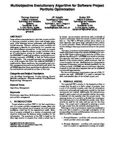
There are two problems for these chaotic maps. One is that the range of ICMIC and Zaslavskii maps is not (0, 1). As a result, the generated chaotic sequences need the scale transformation. Another is some maps, like tent map, have fixed points. Therefore, jumping out from fixed points is necessary for maintaining the chaos characteristics. Figure 1 shows the distribution of different chaotic maps. It reveals that baker’s map, bat map, and tent map have uniform distribution, while other chaotic maps, like circle map, cubic map, ICMIC map, logistic map, and Zaslavskii map, have nonuniform distribution, relatively.

5. Chaotic Multiobjective Evolutionary Algorithm Based on Decomposition 5.1. The Improving Encoding Method for the TTSP. Integrated encoding scheme (IES) proposed by our previous research [1] can use one chromosome to contain the information about both the processing sequence of the tasks and the occupancy of the instruments for each task. It can transform a discrete optimization problem into a continuous optimization problem. Therefore, the encoding efficiency is improved, and the complexity of the genetic manipulations is reduced. Here, we use an example with four tasks and four instruments for illustration of the role of IES. The detail is in Table 2.

Dimensions

Range

2

𝑥 ∈ (0, 1)

2

𝑥𝑘 ∈ (0, 1)

1

(0, 1)

1

(0, 1)

1

(0, 1)

1

[−1, 1]

1

(0, 1)

1

(0, 1)

1

(0, 1)

2

𝑦𝑘 ∈ [−1.0512, 1.0512]

The main concept of the IES is to use the relationships between the decision variables to express the sequence of tasks and use the values of the variables to represent the occupancy of the instruments for each task. This concept is illustrated in Table 3. The entries in the first row are the decision variables, which range between 0 and 1. They are sorted in ascending order. The rank of every variable denotes a test task index in the sequence. Thus, the second row (or the task sequence) is obtained. On the other hand, the instrument assignment can also be obtained from the decision variables. If we want to know which instruments will be occupied by the task 𝑡𝑗 , 𝑤𝑗𝑘 should be ascertained. In other words, we should know the value of 𝑘, which can be calculated by the decision variable corresponding to 𝑡𝑗 . The formula is as follows: 𝑘 = [𝑥𝑖𝑗 × 10] mod 𝑘𝑗 + 1.

(6)

Here, 𝑥𝑖𝑗 ∈ [0, 1] represents the decision variable that corresponds to 𝑡𝑗 , and 𝑘𝑗 is the number of schemes of 𝑡𝑗 . For example, for the task 𝑡1 , the corresponding decision variable is 0.1270, and the number of schemes is 𝑘1 = 2. Then, the value of 𝑘 can be calculated as follows according to (6): 𝑘 = [0.1270 × 10] mod 𝑘1 + 1 = 1 mod 2 + 1 = 2. Therefore, 𝑤12 = {𝑟2 , 𝑟4 } is occupied. However, this encoding scheme has one defect that all schemes are selected with unequal probability. For example,


5

Bakers

1500

Cat

1500

1000

Circle

2000 1500

1000

1000 500 0

500

0

0.5 Cubic

3000

0

1

500 0.5

0

Gauss

1500

2000

1000

1000

500

0

1

0.5

0

1

ICMIC

2000 1500 1000

0

0

0.5

0

1

500 0.5

0

Logistic

3000

Sinusoidal

3000

0

1

2000

1000

1000

1000

500

0

0.5

0

1

0.5

0

0

1

1

Tent

1500

2000

0

0.5

0

0

0.5

1

Zaslavskii

2000 1500 1000 500 0

0.5

0

1

Figure 1: Distribution of different chaotic maps.

for one task 𝑡4 , the number of schemes is 𝑘4 = 3. Then, the value of 𝑘 can be calculated according to (6) as shown in Table 4. As seen from Table 4, the probability of 𝑘 = 1 is 4/10, but 3/10 for 𝑘 = 2, 3. It means all schemes are selected with unequal probability. Based on the original formula, we improved the encoding strategy as follows: 𝑘 = [𝑥𝑖𝑗 𝑘𝑗 × 10] mod 𝑘𝑗 + 1.

(7)

Then, the value of 𝑘 can be calculated according to (7) as shown in Table 5. As seen from Table 5, the equal probability of 𝑘 = 1, 2, 3 is 1/3. This encoding method never generates duplication of a certain task and does not generate unfeasible solutions. In addition, equal probability can maintain impartiality for all

Table 2: A TTSP with four tasks and four instruments. 𝑇 𝑡1 𝑡2 𝑡3 𝑡4

𝑊𝑗 𝑤11 𝑤12 𝑤21 𝑤22 𝑤31 𝑤41 𝑤42 𝑤43

𝑤𝑗𝑘

𝑃𝑗𝑘

𝑟1 , 𝑟2 𝑟2 , 𝑟4 𝑟1 𝑟3 𝑟4 𝑟1 , 𝑟3 𝑟2 , 𝑟4 𝑟2 , 𝑟3

5 3 4 1 2 4 3 7

schemes. It can help the algorithms to match the TTSP with multiple alternative schemes.

6

Mathematical Problems in Engineering Table 3: Example of the integrated encoding scheme.

Decision variables 𝑥𝑖𝑗 Tast sequence 𝑡𝑗 𝑘 𝑤𝑗𝑘 𝑃𝑗𝑘

0.8147 3 1 𝑟4

0.9058 4 1 𝑟1 , 𝑟3

0.1270 1 2 𝑟2 , 𝑟4

0.6324 2 1 𝑟1

2

4

3

4

Table 4: The integrated encoding scheme. Decision variables 𝑥𝑖𝑗 𝑘

[0.0, 0.1) [0.3, 0.4) [0.6, 0.7) [0.9, 1.0)

[0.1, 0.2) [0.4, 0.5) [0.7, 0.8)

[0.2, 0.3) [0.5, 0.6) [0.8, 0.9)

1

2

3

𝑠 = 1, 2, . . . , 𝑁, 𝑖 = 1, 2, . . . , 𝑁. (8)

Here, the initial population is generated by chaos maps. For example, if the sinusoidal map is used for initialization, 𝑥𝑠𝑖+1 = sin(𝜋𝑥𝑠𝑖 ). (2) Crossover. Crossover is the most important step in the process of the evolution. It is directly related to the convergence, diversity, and other performances of the optimal solutions. In this paper, a differential evolution (DE) operator is adopted. In the DE operator, each child individual 𝑥𝑖𝑡+1 is generated as follows: 𝑡 𝑡 𝑥𝑖𝑡 + 𝐹 × (𝑥𝑖1 − 𝑥𝑖2 ) if rand < CR, 𝑥𝑖𝑡 otherwise.

𝑥𝑠∗ = 𝑥𝑠 + (𝑥𝑠𝑢 − 𝑥𝑠𝑙 ) × 𝛿𝑠 ,

(9)

𝑡 𝑡 and 𝑥𝑖2 are Here, CR and 𝐹 are two control parameters. 𝑥𝑖1 𝑡 two individuals chosen in the neighborhood of 𝑥𝑖 . Since 𝐹 is a random number that ranges from 0 to 1, 𝐹 can be generated

(10)

where 𝑥𝑠𝑢 and 𝑥𝑠𝑙 are the upper and lower bounds of 𝑥𝑠 . Consider 1/(𝜂 +1)

(1) Initialization. In order to guarantee the diversity of the initial population, the chaos initialization is applied in this paper. For example, we assume 𝑁 individuals in population, and one of them can be denoted by

𝑥𝑖𝑡+1 = {

(3) Mutation. Mutation operator that prevents solutions from being trapped into local optima is indispensable in the process of the evolution. In this paper, a polynomial mutation operator is adopted. For a solution 𝑥𝑠 , the polynomial mutation is described as

(2𝑢 ) 𝑚 − 1 𝛿𝑠 = { 𝑠 1/(𝜂 +1) 1 − (2 × (1 − 𝑢𝑠 )) 𝑚

5.2. Application of Chaotic Maps in MOEA/D. The multiobjective evolutionary algorithm based on decomposition is originated from Tchebycheff decomposition. It decomposes a multiobjective problem into a number of scalar optimization subproblems and optimizes them simultaneously. Each subproblem is bound with a weight vector and is optimized by using the information from its several neighbor subproblems [20]. In this paper, chaotic variables are used instead of random variables in MOEA/D. Ten chaotic maps are embedded in MOEA/D to replace the random operation. Three key phases in evolutionary algorithms, initialization, crossover, and mutation, are chosen to be embedded with chaos. Different chaotic maps have different formulas and characters. Here, we use sinusoidal map [21] as an example.

𝑥𝑠 = {𝑥𝑠1 , 𝑥𝑠2 , . . . 𝑥𝑠𝑖 , . . . , 𝑥𝑠𝑛 } ,

by chaotic maps instead of random generation. For instance, if the sinusoidal map is used and, in the 𝑖th iteration, 𝐹 = 𝐹𝑖 , then, in the (𝑖 + 1)th iteration, 𝐹𝑠 = 𝐹𝑖+1 = sin(𝜋𝐹𝑖 ).

if 𝑢𝑠 < 0.5, otherwise.

(11)

Here, 𝑢𝑠 is a random number ranging from 0 to 1. 𝜂𝑚 is the distribution index for the mutation operator. Similar to the crossover scheme, we have 𝑢𝑠 = 𝑢𝑖+1 = sin(𝜋𝑢𝑖 ) when using the sinusoidal map.

6. Experiments We carry out four types of experiments to illustrate the performances of the mentioned approaches. Experiment 1 shows the effectiveness of the improving encoding method based on one large scale TTSP. Experiment 2 aims to solve a small scale TTSP benchmark to measure the performance of the evolutionary algorithm using chaotic maps in three phases. Experiment 3 is similar to experiment 2, except that it aims to solve the large scale TTSP. In both experiments 2 and 3, ten chaotic maps are embedded in three different phases in the original MOEA/D algorithm. Each time, only one parameter is modified. The Pareto set (PF) is used to show the effect firstly. Then, the performance metrics HV and 𝐶 are used to further evaluate the performance of chaotic maps embedded algorithm and the original algorithm. Based on the results of the above experiments, we compare the CMOEA/D with the VNM [5] in experiment 4. The parameters for all experiments are shown in Table 6. 𝑛iter is the number of iterations. 𝑛pop is the scale of the population. 𝑛var is the number of decision variables. CR and 𝑃𝑚 (equal to the reciprocal of 𝑛var ) are the probabilities of crossover and mutation operations. 6.1. Experiment 1: The Performance of the Improving Encoding Method. This experiment shows the effectiveness of the improving encoding method in solving the TTSP. The instance is based on a large scale TTSP 40 × 12 [4]. 50 runs of the same experiment have been performed, and the best run among the 50 runs is given in Figure 2. Here, MOEA/D1, MOEA/D-2, and MOEA/D-3 represent the algorithm with different encoding method of random, IES, improving IES separately. We can find from the Pareto front that the improving encoding method obtains better convergence of the solutions of the TTSP. The equal probability also helps the algorithm


7

Table 5: The improving integrated encoding scheme. Decision variables 𝑥𝑖𝑗 /30

[0, 1)[3, 4)[6, 7)[9, 10) [12, 13)[15, 16)[18, 19) [21, 22)[24, 25)[27, 28)

[1, 2)[4, 5)[7, 8)[10, 11) [13, 14)[16, 17)[19, 20) [22, 23)[25, 26)[28, 29)

[2, 3)[5, 6)[8, 9)[11, 12) [14, 15)[17, 18)[20, 21) [23, 24)[26, 27)[29, 30)

1

2

3

𝑘

Table 6: The setting of parameters. 6×8

Mean workload

𝑛iter 𝑛pop 𝑛var CR 𝑃𝑚

20 × 8

30 × 12

40 × 12

30

40

1/30

1/40

250 100 6

20

1/6

1/20

0.9

34 32 30 28 26 24 22 20 18 16 14 35

40

MOEA/D-1 MOEA/D-2

45

50 55 Makespan

60

65

70

MOEA/D-3

Figure 2: Comparison of different encoding methods in solving the TTSP.

to obtain good convergence. Therefore, the improving IES is used in the following experiments because of the efficiency. 6.2. Experiment 2: The Performance for the Small Scale TTSP. This experiment is carried out to show the effectiveness of CMOEA/D for the small scale TTSP 6 × 8. 10 times of the same experiment have been performed, and the best results obtained from original MOEA/D and many variants of CMOEA/D for this instance are shown in Figures 3, 4, and 5. For the convenience, the algorithms with different combinations of chaotic maps and phases are named as “CMOEA/D-[phase][chaotic map].” The ten chaotic maps (baker, cat, circle, cubic, Gauss, ICMIC, logistic, sinusoidal, tent, and Zaslavskii) are denoted by 1, 2, 3, . . . , 10 in alphabetical order. “𝑅” represents the original MOEA/D. “𝐼” represents the phase for initial population. “𝐶” represents the phase for the crossover operator. “𝑀” represents the phase for the mutation operator. For example, the algorithm for initial population by logistic map is named “CMOEA/D-I7.” According to the name role, Figure 3 indicates the performance of the chaotic maps for crossover for solving the TTSP. Figure 4 shows the performance of the chaotic maps

for initialization for solving the TTSP. Figure 5 shows the performance of the chaotic maps for mutation for solving the TTSP. For the small scale TTSP, the performance for convergence is not very obvious from the Pareto set. The solutions obtained from the original algorithm and the chaos embedded algorithm overlap each other. However, the diversity of the solutions obtained from the chaos embedded algorithm is better than the original algorithm. 6.3. Experiment 3: The Performance for the Large Scale TTSP. This experiment is carried out to show the effectiveness of CMOEA/D for three large scale problems, TTSP 20 × 8, 30 × 12, and 40 × 12. 10 times of the same experiment have been performed, and the best results obtained from original MOEA/D and many variants of CMOEA/D are shown in Figures 6, 7, 8, 9, 10, 11, 12, 13, and 14. The name role of the figures is similar to the small scale instance. For the large scale TTSP, both the convergence and diversity of solutions are improved significantly. Almost every chaotic map has good performance for the improvement, but the performance is not stable and positive for some chaotic maps. For example, the tent, baker, and cat maps even have negative effects for the solutions under some situations. 6.4. Performance Analysis. Based on the above experiments, we use the statistical data of the comprehensive metric HV and convergence metric 𝐶 to indicate the results from different aspects, because the figure of Pareto front can provide only the primary idea but not the comprehensive effect. The conclusion about the guidance of chaotic maps for resolving the TTSP will be investigated based on these data. 6.4.1. Performance Metrics (1) Hypervolume (see [11]). This quality indicator calculates the volume (in the objective space) covered by members of a nondominated set of solutions for problems where all objectives are to be minimized. Mathematically, for each solution 𝑖 ∈ 𝑆, a hypercube V𝑖 is constructed with a reference point 𝑊 and the solution 𝑖 as the diagonal corners of the hypercube. The reference point can simply be found by constructing a vector of worst objective function values. Thereafter, a union of all hypercubes is found and its hypervolume is calculated as follows:

HV (𝑆) = Leb (⋃ V𝑖 ) . 𝑖∈𝑆

(12)

8


Baker

Mean workload

25

Cat

25

20

20

20

15

15

15

10 20

25

30

35

40

45

10 20

25

Makespan MOEA/D CMOEA/D-C1

Mean workload

35

40

10 20

Gauss

25

20

15

15

15

30 35 Makespan

40

45

10 20

30

35

40

45

10

20

MOEA/D CMOEA/D-C5

Logistic

Sinusoidal

25

20

15

15

15

35 30 Makespan

40

45

10 20

25

30

35

40

45

10 20

Makespan

MOEA/D CMOEA/D-C7

Zaslavskii

Mean workload

20

15

10

20

25

45

40

45

40

45

30 Makespan

Tent

25

30 35 Makespan

MOEA/D CMOEA/D-C9

MOEA/D CMOEA/D-C8 25

30 35 Makespan

25

20

25

40

MOEA/D CMOEA/D-C6

20

10 20

25

Makespan


25

30 35 Makespan

ICMIC

25

20

25

25

MOEA/D CMOEA/D-C3

20

10 20

Mean workload

30 Makespan

MOEA/D CMOEA/D-C2 Cubic

25

Circle

25

35

40

MOEA/D CMOEA/D-C10

Figure 3: Comparison of different chaotic maps for crossover.

Mathematical Problems in Engineering Baker

25 Mean workload

9 Cat

25

20

20

20

15

15

15

10 20

25

30 Makespan

35

40

10 20

MOEA/D CMOEA/D-I1

Mean workload

35

40

10 20

Gauss

25

20

15

15

15

25

30

35

40

45

10 20

25

Makespan

Logistic

25

30 35 Makespan

40

45

10

20

20

15

15

15

25

30 Makespan

35

40

10

20

25

30

25

20

35

40

45

10 20

25

Zaslavskii

Mean workload

20

15

10

20

25

30

30 Makespan

MOEA/D CMOEA/D-I9

MOEA/D CMOEA/D-I8 25

40

45

Tent

Makespan

MOEA/D CMOEA/D-I7

30 35 Makespan

25

20

10 20

40

MOEA/D CMOEA/D-I6

Sinusoidal

25

35

ICMIC

MOEA/D CMOEA/D-I5

MOEA/D CMOEA/D-I4

30 Makespan

25

20

20

25

MOEA/D CMOEA/D-I3

20

10

Mean workload

30 Makespan

MOEA/D CMOEA/D-I2 Cubic

25

25

Circle

25

35

40

45

Makespan MOEA/D CMOEA/D-I10

Figure 4: Comparison of different chaotic maps for initialization.

35

40

10


Mean workload

25

Cat

25

20

20

20

15

15

15

10 20

25

30 Makespan

35

40

10

20

MOEA/D CMOEA/D-M1

Mean workload

40

45

10

20

15

15

15

30 35 Makespan

40

45

10 20

MOEA/D CMOEA/D-M4

30 35 Makespan

40

45

10 20

Sinusoidal

25

20

20

15

15

15

25

35 30 Makespan

40

45

10

20

MOEA/D CMOEA/D-M7

25

30 35 Makespan

40

45

10

20

Zaslavskii

Mean workload

15

20

25

30 35 Makespan

25

30 35 Makespan

MOEA/D CMOEA/D-M9

20

10

35 30 Makespan

40

45

40

45

Tent

MOEA/D CMOEA/D-M8 25

25

25

20

10 20

45

MOEA/D CMOEA/D-M6

MOEA/D CMOEA/D-M5

Logistic

25

25

40

ICMIC

25

20

25

30 35 Makespan

MOEA/D CMOEA/D-M3

Gauss

25

25

20

20

10 20

Mean workload

35 30 Makespan

MOEA/D CMOEA/D-M2

Cubic

25

25

Circle

25

40

45

MOEA/D CMOEA/D-M10

Figure 5: Comparison of different chaotic maps for mutation.


Baker

18 Mean workload

11

16

14

12 30

40

50

Cat

20

60

70

18

18

16

16

14

14

12 30

40

50

Mean workload

80

12 30

Cubic

20

18

14

15

16

40

60 Makespan

80

100

10 30

Logistic

70

80

20

30

15

20

50

14

40

30

50 Makespan

60

70

80

100

MOEA/D CMOEA/D-C6

Sinusoidal

40

Tent

30 25 20

10 30

40

50

60

70

15

10 30

40

Makespan

60

50

10 20

40

Makespan

MOEA/D CMOEA/D-C7

MOEA/D CMOEA/D-C8

18 16 14 12 30

40

50 Makespan

60 Makespan

MOEA/D CMOEA/D-C9

Zaslavskii

20 Mean workload

Mean workload

50 60 Makespan

MOEA/D CMOEA/D-C5


40

45

ICMIC

20

16

12 20

40

MOEA/D CMOEA/D-C3 Gauss

25

35

Makespan

MOEA/D CMOEA/D-C2

MOEA/D CMOEA/D-C1

18

70

60 Makespan

Makespan

Circle

20

60

70

MOEA/D CMOEA/D-C10

Figure 6: Comparison of different chaotic maps for crossover for 20 × 8.

12


Mean workload

20

18

16

14 30

35

Cat

20

40 Makespan

45

50

18

18

16

16

14

14

12 30

Cubic

20 Mean workload

50 Makespan

60

70

Gauss

60 80 Makespan

100

120

ICMIC

20 18

18

16

16 16

14 40

60 Makespan

80

100

14

14 30

Logistic

20

40 Makespan

35

45

50

12 30

MOEA/D CMOEA/D-I5

MOEA/D CMOEA/D-I4

Sinusoidal

25

18

16

15

16

40

45

50

10 30

40

MOEA/D CMOEA/D-I7

60

50 Makespan

Makespan

70

Mean workload

14 30

35

Zaslavskii

18 16 14 12 30

40

50 Makespan

60

70

Tent

40 45 Makespan

MOEA/D CMOEA/D-I9

MOEA/D CMOEA/D-I8 20

50 Makespan

20

20

35

40

MOEA/D CMOEA/D-I6

18

14 30

40

MOEA/D CMOEA/D-I3

20

18

12 20

12 20

MOEA/D CMOEA/D-I2

MOEA/D CMOEA/D-I1

Mean workload

40

Circle

20

60

70

MOEA/D CMOEA/D-I10

Figure 7: Comparison of different chaotic maps for initialization for 20 × 8.

50

55


25

Mean workload

13 Cat

20

18

18

20

16 16

15

10 30

40

50

60

70

14 30

14 40

Makespan

Mean workload

60

70

12 30

Gauss

20

18

16

16

16

14

14

14

60 Makespan

80

100

12 30

60 50 Makespan

70

80

12 30

Logistic

20

20

15

15

15

35

40

45

50

55

10 20

30

Makespan MOEA/D CMOEA/D-M7

40 50 Makespan

60

70

10 30

40

16 14 35

40 Makespan

50

MOEA/D CMOEA/D-M9

18

12 30

60

70

60

70

Tent

Zaslavskii

20

50

Makespan

MOEA/D CMOEA/D-M8

Mean workload

40

25

20

10 30

55

MOEA/D CMOEA/D-M6

Sinusoidal

25

50

Makespan

MOEA/D CMOEA/D-M5


40

45

ICMIC

20

18

40

40

MOEA/D CMOEA/D-M3

18

12 20

35

Makespan

MOEA/D CMOEA/D-M2 Cubic

20

50 Makespan

MOEA/D CMOEA/D-M1

Mean workload

Circle

20

45

50

MOEA/D CMOEA/D-M10

Figure 8: Comparison of different chaotic maps for mutation for 20 × 8.

14


Baker

Mean workload

20

20

20

16

15

18

40

50 60 Makespan

70

80

10 20

Mean workload

60

80

100

16 20

40

Makespan

MOEA/D CMOEA/D-C1

22

80

100

MOEA/D CMOEA/D-C3

Gauss

25

60 Makespan

MOEA/D CMOEA/D-C2

Cubic

24

40

Circle

22

18

14 30

ICMIC

22

20

20

15

18

20 18 16 30

60 50 Makespan

40

70

80

10 30

50

60

70

16 30

40

70

80

70

80

MOEA/D CMOEA/D-C6

Sinusoidal

24

60

50

Makespan

MOEA/D CMOEA/D-C5

Logistic

25

40

Makespan

MOEA/D CMOEA/D-C4

Tent

25

22 20

20

20

18 15 30

40

50 Makespan

60

70

16 30

MOEA/D CMOEA/D-C7

40

60 50 Makespan

70

80

15 30

40

MOEA/D CMOEA/D-C9

Zaslavskii

25

20

15 30

40

50 60 Makespan

50

60

Makespan

MOEA/D CMOEA/D-C8

Mean workload

Mean workload

Cat

25

70

80

MOEA/D CMOEA/D-C10



24 Mean workload

15

22

25

25

18

20

20

40

60 Makespan

80

100

15 20

40

60 Makespan

80

100

15 30

MOEA/D CMOEA/D-I2

MOEA/D CMOEA/D-I1

Cubic

25

Gauss

30

40

50 60 Makespan

70

80

MOEA/D CMOEA/D-I3 ICMIC

25

25 20

20 20

15

30

40

50

60

70

80

15

30

60

70

15

20

40

Makespan

MOEA/D CMOEA/D-I4

22

80

100

MOEA/D CMOEA/D-I6

Sinusoidal

25

60 Makespan

MOEA/D CMOEA/D-I5 Logistic

24

50

40

Makespan

Tent

30

20

25

15

20

20 18 16

20

40

60 Makespan

80

100

10 30

40

50

60

70

80

15

30

40

Makespan

MOEA/D CMOEA/D-I7

Zaslavskii

25

20

15 20

40

60 Makespan

50 60 Makespan

MOEA/D CMOEA/D-I9

MOEA/D CMOEA/D-I8

Mean workload

Mean workload

Circle

30

20

16 20

Mean workload

Cat

30

80

100

MOEA/D CMOEA/D-I10


70

80

16


Mean workload

25

Cat

25

20 20

20

15 15 30

40

50 60 Makespan

70

15 30

80

40

Cubic

Mean workload

30

50 60 Makespan

70

80

10 30

20

20

20

18

18

15

16

16

20

40

60 Makespan

80

100

14

30

50

60

70

80

14

Sinusoidal

22

25

16

18

20

60

70

80

16

30

40

50 60 Makespan

Makespan MOEA/D CMOEA/D-M7

70

80

15 30

Mean workload

40

16

40

50

MOEA/D CMOEA/D-M9 Zaslavskii

20

70

80

70

80

Tent

18

14

60

60 Makespan

60

Makespan


50

30

20

50

40

MOEA/D CMOEA/D-M6

MOEA/D CMOEA/D-M5

Logistic

70

Makespan

18

14 40

30

Makespan


40

60

ICMIC

22

25

10

50

MOEA/D CMOEA/D-M3 Gauss

22

40

Makespan

MOEA/D CMOEA/D-M2

MOEA/D CMOEA/D-M1

Mean workload

Circle

25

80

100

MOEA/D CMOEA/D-M10



25 Mean workload

17

20

15 40

50

60 Makespan

70

80

20

20

18

18

16

16 40

Mean workload

70 60 Makespan

80

90

14 40

Gauss

24

22

20

20

20

18

18

18

60 70 Makespan

80

90

16 40

60

70

80

90

MOEA/D CMOEA/D-C5

Logistic

50

60

70

80

90

80

90

MOEA/D CMOEA/D-C6

Sinusoidal

25

80

Makespan

Tent

24 22

22 20

20

20

18

18 50

60 70 Makespan

80

90

15 40

60

80

100

16 40

50

Makespan

MOEA/D CMOEA/D-C7

MOEA/D CMOEA/D-C9

Zaslavskii

24 22 20 18 16 40

50

60

60

70

70

Makespan

MOEA/D CMOEA/D-C8

Mean workload

16 40

16 40

Makespan


50

70

ICMIC

24

22

50

60

MOEA/D CMOEA/D-C3

MOEA/D CMOEA/D-C2 Cubic

50

Makespan

22

16 40

Mean workload

50

Circle

22

22

MOEA/D CMOEA/D-C1

24

Cat

24

80

90

Makespan MOEA/D CMOEA/D-C10


18


Baker

Mean workload

24 22

22

20

20

18

18

16

40

50

60

Cat

24

70

80

90

20

16 40

60

Cubic

Mean workload

20

20

18

18

16

Gauss

80

60

100

14 40

Logistic

50

60 70 Makespan

80

90

70

80

15 40

20

18

18

16

16 40

50

50

60 70 Makespan

80

90

MOEA/D CMOEA/D-I8

80

14 40

45

50

50 55 Makespan

MOEA/D CMOEA/D-I9

20

40

80

90

60

65

Tent

Zaslavskii

25

60 70 Makespan

22 20

15

70

MOEA/D CMOEA/D-I6

22

MOEA/D CMOEA/D-I7

Mean workload

Mean workload

60 Makespan

Sinusoidal

24

20

60 Makespan

ICMIC

25

MOEA/D CMOEA/D-I5

MOEA/D CMOEA/D-I4

50

50

20

Makespan

15 40

15 40

MOEA/D CMOEA/D-I3

22

22

25

100

MOEA/D CMOEA/D-I2

MOEA/D CMOEA/D-I1

16 40

80 Makespan

Makespan

24

Circle

25

60

70

80

90

Makespan MOEA/D CMOEA/D-I10



Baker

25 Mean workload

19

20

20

20

18

50

60 70 Makespan

80

90

16 40

MOEA/D CMOEA/D-M1

50

60 70 Makespan

80

90

15 40

22

60

70

80

MOEA/D CMOEA/D-M3

Gauss

30

50

Makespan

MOEA/D CMOEA/D-M2

Cubic

24

Mean workload

Circle

25

22

15 40

ICMIC

30

25

25

20

20

20 18 16 40

50

60 70 Makespan

80

90

15 40

Logistic

24

22

20

20

18

18

50

70 60 Makespan

60 70 Makespan

80

90

15 40

80

90

16 40

MOEA/D CMOEA/D-M7

80

90

Tent

20

50

60 70 Makespan

80

90

15 40

50

20

18

50

60 Makespan

60 Makespan

MOEA/D CMOEA/D-M9

Zaslavskii

22

16 40

60 70 Makespan

25

MOEA/D CMOEA/D-M8

Mean workload

50

MOEA/D CMOEA/D-M6

Sinusoidal

24

22

16 40

50

MOEA/D CMOEA/D-M5

MOEA/D CMOEA/D-M4

Mean workload

Cat

24

70

80

MOEA/D CMOEA/D-M10


70

80

20

Mathematical Problems in Engineering TTSP 20 ∗ 8

1 0.8

0.6

0.6

C-measure

0.8 0.4 0.2

0.4

0

0

−0.2

−0.2

+ + +

(R, I1) (I1, R) (R, I2) (I2, R) (R, I3) (I3, R) (R, I4) (I4, R) (R, I5) (I5, R) (R, I6) (I6, R) (R, I7) (I7, R) (R, I8) (I8, R) (R, I9) (I9, R) (R, I10) (I10, R)

Algorithm

Algorithm

Figure 15: The boxplots of 𝐶 for chaotic maps embedded in crossover.

Figure 16: The boxplots of 𝐶 for chaotic maps embedded in initialization.

Here, Leb denotes the Lebesgue measure. Algorithms with larger values of HV are desirable.

1

TTSP 20 ∗ 8 +

0.8 C-measure

(2) Coverage Metric 𝐶 (see [11]). The metric 𝐶 can be used to compare the performances of the two-solution sets. Assume 𝐴 and 𝐵 are two sets of nondominated solutions. 𝐶(𝐴, 𝐵) represents the proportion of points in set 𝐵 dominated over 𝐴 in the total points in set 𝐵. Consider

0.6 0.4 0.2 0 −0.2

(13)

The value 𝐶(𝐴, 𝐵) = 1 means that all of the solutions in 𝐵 are dominated by solutions in 𝐴, while 𝐶(𝐴, 𝐵) = 0 means that no solution in 𝐵 is dominated by a solution in 𝐴. Note that both the 𝐶(𝐴, 𝐵) and 𝐶(𝐵, 𝐴) have to be considered for comprehensive dominated information for comparing the different set obtained from different algorithm, because 𝐶(𝐴, 𝐵) ≠ 1 − 𝐶(𝐵, 𝐴). 6.4.2. Experiment Results. The average values of performance metrics HV and 𝐶 of 10 independent runs for both the small and the large scale TTSPs are in Tables 7 and 8, respectively. The symbol is similar to the above mentioned role. In all of the cases, the best performances are denoted in bold. As shown in Tables 7 and 8, most of the combinations of chaotic maps with MOEA/D have a positive effect for both the small scale and the large scale instances. However, the larger the scale is, the weaker the chaos effect is. In most cases, the best performance in Table 7 is consistent with that in Table 8. It means the chaotic maps in the specific location have better convergence and comprehensive performances simultaneously. In fact, metric HV and metric 𝐶 are different aspects to evaluate the algorithm. Therefore, some inconsistences exist also. Here, we represent the statistical results in an intuitive way. If both the convergence and the comprehensive performances of the algorithm with chaotic maps are better than the original algorithm, the value is replaced by “++.” When the situation is opposite, blank is used to replace the corresponding value. Table 9 shows the results.

(R, M1) (M1, R) (R, M2) (M2, R) (R, M3) (M3, R) (R, M4) (M4, R) (R, M5) (M5, R) (R, M6) (M6, R) (R, M7) (M7, R) (R, M8) (M8, R) (R, M9) (M9, R) (R, M10) (M10, R)

󵄨 󵄨󵄨 󵄨{𝑥 ∈ 𝐵 | ∃𝑦 ∈ 𝐴 : 𝑦 dominates 𝑥}󵄨󵄨󵄨 . 𝐶 (𝐴, 𝐵) = 󵄨 |𝐵|

TTSP 20 ∗ 8

0.2

(R, C1) (C1, R) (R, C2) (C2, R) (R, C3) (C3, R) (R, C4) (C4, R) (R, C5) (C5, R) (R, C6) (C6, R) (R, C7) (C7, R) (R, C8) (C8, R) (R, C9) (C9, R) (R, C10) (C10, R)

C-measure

1

Algorithm

Figure 17: The boxplots of 𝐶 for chaotic maps embedded in mutation.

The results show that circle map and ICMIC map in all phases especially in crossover operator have the best performance. Cubic map and logistic map in mutation operator, Gauss map in crossover operator and mutation operator, sinusoidal map in crossover operator and initial population, baker’s map in crossover operator, and Zaslavskii map in initial population have a better effect. In addition, cat map in initial population and mutation operator also has a little bit of effect. In order to show the above results in an intuitive way, the boxplots of the performance metric 𝐶 are also adopted to illustrate the same conclusion. Here, we use the boxplots for TTSP 20 × 8 as an example. The name role is similar to the above mentioned principle. The ten chaotic maps (baker, cat, circle, cubic, Gauss, ICMIC, logistic, sinusoidal, tent, and Zaslavskii) are denoted by 1, 2, 3, . . . , 10 in alphabetical order. In addition, “𝑅” represents the original MOEA/D. “𝐼” represents the phase for initial population. “𝐶” represents the phase for crossover operator. “𝑀” represents the phase for mutation operator. For example, the algorithm for initial population by logistic map is named “I7.” Figures 15, 16, and 17 are the boxplots for chaotic maps embedded in crossover, in initialization, and in mutation, separately.


21 Table 7: The average value of HV.

Baker Cat Circle Cubic Gauss ICMIC Logistic Sinusoidal Tent Zaslavskii

𝑅 0.3312 0.3312 0.3312 0.3312 0.3312 0.3312 0.3312 0.3312 0.3312 0.3312

𝐶 0.3555 0.3361 0.3514 0.3536 0.3470 0.3618 0.3450 0.3514 0.3566 0.3276


𝑅 0.5326 0.5326 0.5326 0.5326 0.5326 0.5326 0.5326 0.5326 0.5326 0.5326

𝐶 0.4976 0.5283 0.5350 0.5164 0.5167 0.5428 0.5261 0.5152 0.5312 0.4911

6×8 𝑅 𝐼 0.3312 0.3240 0.3312 0.3592 0.3312 0.3538 0.3312 0.3305 0.3312 0.3324 0.3312 0.3416 0.3312 0.3302 0.3312 0.3373 0.3312 0.3318 0.3312 0.3376 30 × 12 𝑅 𝐼 0.5326 0.5515 0.5326 0.5484 0.5326 0.5160 0.5326 0.5314 0.5326 0.5194 0.5326 0.5105 0.5326 0.5458 0.5326 0.5201 0.5326 0.5380 0.5326 0.5028

𝑅 0.3312 0.3312 0.3312 0.3312 0.3312 0.3312 0.3312 0.3312 0.3312 0.3312

𝑀 0.3716 0.3429 0.3528 0.3511 0.3568 0.3672 0.3394 0.3386 0.3416 0.3434

𝑅 0.7471 0.7471 0.7471 0.7471 0.7471 0.7471 0.7471 0.7471 0.7471 0.7471

𝐶 0.7724 0.7460 0.7502 0.7411 0.7538 0.7557 0.7579 0.7540 0.7442 0.7466

𝑅 0.5326 0.5326 0.5326 0.5326 0.5326 0.5326 0.5326 0.5326 0.5326 0.5326

𝑀 0.5398 0.5708 0.5357 0.5195 0.5176 0.5475 0.5155 0.5181 0.5187 0.5150

𝑅 0.7588 0.7588 0.7588 0.7588 0.7588 0.7588 0.7588 0.7588 0.7588 0.7588

𝐶 0.9734 0.7777 0.8077 0.7576 0.7513 0.8214 0.7360 0.7904 0.7600 0.7506

20 × 8 𝑅 𝐼 0.7471 0.7472 0.7471 0.7580 0.7471 0.7556 0.7471 0.7448 0.7471 0.7294 0.7471 0.7465 0.7471 0.7560 0.7471 0.7483 0.7471 0.7486 0.7471 0.7562 40 × 12 𝑅 𝐼 0.7588 0.7168 0.7588 0.7289 0.7588 0.7250 0.7588 0.7551 0.7588 0.7726 0.7588 0.7370 0.7588 0.7064 0.7588 0.6875 0.7588 0.7144 0.7588 0.8685

𝑅 0.7471 0.7471 0.7471 0.7471 0.7471 0.7471 0.7471 0.7471 0.7471 0.7471

𝑀 0.7480 0.7370 0.7608 0.7595 0.7548 0.7488 0.7539 0.7547 0.7448 0.7433

𝑅 0.7588 0.7588 0.7588 0.7588 0.7588 0.7588 0.7588 0.7588 0.7588 0.7588

𝑀 0.7395 0.8604 0.7538 0.7357 0.7353 0.7569 0.7796 0.7440 0.7881 0.8432

(𝑅, 𝑀) 0.3815 0.4660 0.2672 0.2964 0.2475 0.2637 0.2338 0.3333 0.3911 0.3490

(𝑀, 𝑅) 0.3572 0.1102 0.4786 0.3158 0.4288 0.3743 0.4438 0.3158 0.2708 0.2720

(𝑅, 𝑀) 0.4676 0.4573 0.3883 0.4272 0.3629 0.3899 0.3341 0.4354 0.3538 0.4932

(𝑀, 𝑅) 0.3046 0.2652 0.3801 0.3358 0.3899 0.3902 0.4106 0.4003 0.4387 0.3487

Table 8: The average value of 𝐶.


(𝑅, 𝐶) 0.0400 0.0000 0.0500 0.0900 0.0250 0.0000 0.0900 0.0250 0.0000 0.0000

(𝐶, 𝑅) 0.0583 0.0000 0.0833 0.0833 0.1083 0.0583 0.0583 0.0500 0.0750 0.0000


(𝑅, 𝐶) 0.5861 0.4136 0.2573 0.4172 0.4304 0.3204 0.3935 0.4075 0.3002 0.6872

(𝐶, 𝑅) 0.2929 0.3699 0.4552 0.2880 0.3084 0.5210 0.3342 0.4172 0.3803 0.1425

6×8 (𝑅, 𝐼) (𝐼, 𝑅) 0.0400 0.0000 0.0000 0.0667 0.0367 0.0917 0.0250 0.0583 0.0250 0.0250 0.0450 0.0833 0.0250 0.0583 0.0500 0.0583 0.0500 0.0000 0.0000 0.0333 30 × 12 (𝑅, 𝐼) (𝐼, 𝑅) 0.5208 0.2383 0.4242 0.3134 0.4339 0.3152 0.4579 0.3487 0.4930 0.2412 0.5540 0.2483 0.5051 0.2571 0.5211 0.2960 0.4465 0.3732 0.5136 0.3129

(𝑅, 𝑀) 0.0000 0.0000 0.0250 0.0750 0.0250 0.0250 0.0000 0.0500 0.0250 0.0250

(𝑀, 𝑅) 0.1000 0.0250 0.0500 0.0833 0.0833 0.0833 0.0250 0.0250 0.0833 0.0250

(𝑅, 𝐶) 0.1753 0.2800 0.2496 0.3770 0.2982 0.3017 0.1479 0.2652 0.4352 0.2804

(𝐶, 𝑅) 0.5005 0.3847 0.3992 0.3111 0.4293 0.3641 0.4037 0.3502 0.2210 0.2911

(𝑅, 𝑀) 0.4730 0.3993 0.3287 0.3989 0.4560 0.4886 0.4668 0.4670 0.4913 0.5040

(𝑀, 𝑅) 0.4039 0.4263 0.3220 0.3229 0.3533 0.3886 0.3420 0.3727 0.2751 0.3512

(𝑅, 𝐶) 0.2847 0.5515 0.4333 0.4228 0.3788 0.3237 0.4870 0.4508 0.4500 0.3968

(𝐶, 𝑅) 0.4455 0.2536 0.4729 0.2989 0.3788 0.4530 0.3450 0.3314 0.2876 0.3680

20 × 8 (𝑅, 𝐼) (𝐼, 𝑅) 0.3741 0.3233 0.2873 0.3517 0.2713 0.3785 0.2801 0.3596 0.4517 0.1346 0.3097 0.3347 0.2874 0.3465 0.3466 0.4186 0.2500 0.3592 0.3236 0.2762 40 × 12 (𝑅, 𝐼) (𝐼, 𝑅) 0.6541 0.1514 0.5098 0.1996 0.4678 0.3517 0.5586 0.2629 0.5212 0.4023 0.6220 0.2232 0.5793 0.2007 0.7251 0.1100 0.5798 0.2495 0.2626 0.5035

22

Mathematical Problems in Engineering Table 9: The visualized result. 𝐶 ++


6×8 𝐼

++

++ ++

++ ++

++

++ ++

𝑀 ++ ++ ++ ++ ++ ++ ++

++

𝐶 ++ ++ ++ ++ ++ ++

++

20 × 8 𝐼 ++ ++

++ ++ ++

++ TTSP 6 ∗ 8

Mean workload

35 30 25 20 15 30

𝐶

𝑀

𝐶 ++

++ ++ ++ ++ ++

++

++

++

++

40 × 12 𝐼

𝑀

++

++ ++ ++

40

25

30 × 12 𝐼

𝑀

35

40

45

Makespan Solutions

Figure 18: Exhaustive result for TTSP 6 × 8.

Overall, chaotic maps for crossover and mutation operators are helpful for preventing the solutions from trapping in the local optima and have significant improvement on the evolutionary algorithms based on the decomposition for solving the TTSP. Circle map and ICMIC map have the best performance in ten maps especially. Cubic map, logistic map, Gauss map, and sinusoidal map have better contribution in solving those TTSPs. 6.4.3. Result Analysis. We discuss and explore the reason for these conclusions based on the above results. We focus on the distribution of solutions of the TTSP. We calculate the feasible solutions of a small scale TTSP 6 × 8 using the method of enumeration that cannot be used in large scale TTSPs. The result is shown in Figure 18. The solutions for the true Pareto front are [(23, 70/3); (28, 19.5); (31, 18); (36, 14.6)] out of 103,680 solutions in objective space. We can find that the TTSP has nonuniform distribution, and many local optima exist among all the solutions of the TTSP. The chaotic map has the nature to avoid becoming trapped in local optima. The TTSP has many local optima. All the experiments illustrate the fact that using chaotic maps embedded with the evolutionary algorithm can help the TTSP to obtain good solutions. In addition, the process of

crossover and mutation is important for jumping out of local optima. The experiments also validate this fact. Furthermore, chaotic maps have a superior effect on escaping from local optima, but not all of them are effective. We want to find the relationship from the distribution. The distribution of every chaotic map is shown in Figure 1. Some chaotic maps, like circle map, cubic map, and ICMIC map, are relatively nonuniformly distributed. It is very similar to the distribution of the optimal solution of the TTSP. The above experiments indicate that these chaotic maps have a positive effect on TTSP. Some chaotic maps, like cat map, have uniform distribution. The experiments show that they cannot obtain good effect for solving the TTSP in most situations. It is natural that the effect of chaotic maps is floating under different circumstance, because of the ergodicity and stochasticity of chaotic maps. However, the similarity degree of the distribution between the chaotic maps and the problem is a very essential factor for the application of chaotic maps.

6.5. Experiment 4: Comparison of CMOEA/D and VNM. Referring to Table 9, together with the data in Tables 7 and 8, we select a few variants of CMOEA/D to compare with VNM. VNM has been proved to be more suitable to solve the TTSP than other methods such as chaotic NSGA-II (CNSGA) [5]. Therefore, a comparison of CMOEA/D and VNM is carried out to illustrate the performance of our algorithm. We take TTSP 20 × 8 and 40 × 12 as representative test problems. For TTSP 20 × 8, we select the three variants of CMOEA/D. They are CMOEA/D-C1 with baker’s map in crossover operator, CMOEA/D-I9 with tent map in the initial population, and CMOEA/D-M3 with circle map in the mutation operator, respectively. For TTSP 40 × 12, the three variants of CMOEA/D are CMOEA/D-C1 with baker’s map in crossover operator, CMOEA/D-I10 with Zaslavskii map in the initial population, and CMOEA/D-M9 with tent map in the mutation operator, respectively. The results of the performance metrics HV and 𝐶 of 10 independent runs are in Tables 10 and 11, separately. The best results obtained from VNM and three variants of CMOEA/D for different instances are shown in Figures 19 and 20. “𝑉” represents the VNM, and the symbol in the table is similar to the above mentioned role.


23

18

Mean workload

Mean workload

17 16 15 14 13 12 30

40

50

60

24

19

22

18

20

17

18

16

16

15

14

14

12 30

70

Mean workload

19

40

Makespan

50 60 Makespan

13 20

70

VNM CMOEA/D-I9

VNM CMOEA/D-C1

40

60 80 Makespan

100

120

VNM CMOEA/D-M3

Figure 19: Comparison of VNM and three variants of CMOEA/D for 20 × 8.

28

28

26

26

40

35

Mean workload

Mean workload

22 20

Mean workload

24

24

22 20

18

18

16

16

30

25

20

14 40

50

60 70 Makespan

VNM CMOEA/D-C1

80

14 40

50

60

70

Makespan VNM CMOEA/D-I10

80

90

15 40

60

80 100 120 140 160 Makespan

VNM CMOEA/D-M9

Figure 20: Comparison of VNM and three variants of CMOEA/D for 40 × 12.

It shows that the solutions obtained by the CMOEA/D dominate most of the solutions obtained by the VNM in the above figures. The values of 𝐶 in Table 11 indicate that CMOEA/D has good convergence. The results in Table 10 also show that the solutions obtained by CMOEA/D are of higher

comprehensive performance. Therefore, the CMOEA/D has the best performance completely. A short summary can be obtained according to the above experiments and analyses. The improving encoding method is effective for solving the TTSP. In addition, the

24

Mathematical Problems in Engineering Table 10: The value of HV.

1 2 3 4 5 6 7 8 9 10 Average Times

𝑉 0.4067 0.4018 0.4552 0.4258 0.4283 0.4492 0.4560 0.4306 0.4460 0.4458 0.4345 1

𝐶 0.4928 0.4844 0.4776 0.4907 0.5055 0.4690 0.4540 0.4765 0.4872 0.4897 0.4827 9

20 × 8 𝑉 𝐼 0.4067 0.4582 0.4018 0.4756 0.4552 0.4582 0.4258 0.4789 0.4283 0.4607 0.4492 0.4738 0.4560 0.4612 0.4306 0.4688 0.4460 0.4632 0.4458 0.4803 0.4345 0.4679 0 10

𝑉 0.4067 0.4018 0.4552 0.4258 0.4283 0.4492 0.4560 0.4306 0.4460 0.4458 0.4345 0

𝑀 0.4642 0.4746 0.4706 0.4643 0.4755 0.4889 0.4871 0.4789 0.4740 0.4767 0.4755 10

𝑉 0.4016 0.4148 0.4729 0.3881 0.4010 0.4155 0.3900 0.3968 0.4235 0.4002 0.4104 0

𝐶 0.4718 0.4511 0.4729 0.4853 0.4598 0.4389 0.4521 0.4426 0.4585 0.4406 0.4574 9

40 × 12 𝑉 𝐼 0.4016 0.4576 0.4148 0.4449 0.4729 0.4937 0.3881 0.4521 0.4010 0.4674 0.4155 0.4496 0.3900 0.4688 0.3968 0.4703 0.4235 0.4500 0.4002 0.4465 0.4104 0.4601 0 10

𝑉 0.4016 0.4148 0.4729 0.3881 0.4010 0.4155 0.3900 0.3968 0.4235 0.4002 0.4104 1

𝑀 0.4189 0.4521 0.4222 0.4286 0.4666 0.4354 0.4578 0.4750 0.4468 0.4537 0.4457 9

(𝐶, 𝑉) 1.0000 1.0000 1.0000 1.0000 1.0000 0.8571 1.0000 1.0000 1.0000 1.0000 0.9857 10

40 × 12 (𝑉, 𝐼) (𝐼, 𝑉) 0.0000 1.0000 0.0000 1.0000 0.0000 1.0000 0.0000 1.0000 0.0000 1.0000 0.0000 1.0000 0.0000 1.0000 0.0000 1.0000 0.0000 0.7778 0.0000 1.0000 0.0000 0.9778 0 10

(𝑉, 𝑀) 0.0000 0.0000 0.0000 0.0000 0.0000 0.1000 0.0000 0.0000 0.0000 0.0000 0.0100 0

(𝑀, 𝑉) 0.9000 1.0000 1.0000 1.0000 1.0000 0.8571 1.0000 1.0000 0.7778 1.0000 0.9535 10

Table 11: The value of 𝐶.

1 2 3 4 5 6 7 8 9 10 Average Times

(𝑉, 𝐶) 0.0000 0.0000 0.0000 0.0000 0.0000 0.0000 0.4444 0.0000 0.0000 0.0000 0.0444 1

(𝐶, 𝑉) 1.0000 1.0000 0.9000 1.0000 1.0000 0.1667 0.0000 1.0000 1.0000 1.0000 0.8067 9

20 × 8 (𝑉, 𝐼) (𝐼, 𝑉) 0.0000 0.8333 0.0000 1.0000 0.3750 0.5000 0.0000 1.0000 0.0000 0.9000 0.0833 0.1667 0.0000 0.2000 0.0000 1.0000 0.0000 1.0000 0.1000 0.5714 0.0558 0.7171 0 10

(𝑉, 𝑀) 0.0000 0.0000 0.1667 0.0000 0.0000 0.0000 0.0000 0.0000 0.0000 0.0833 0.0250 0

(𝑀, 𝑉) 1.0000 1.0000 0.7000 1.0000 1.0000 1.0000 1.0000 1.0000 1.0000 0.5714 0.9271 10

effectiveness of the multiobjective evolutionary algorithm based on decomposition using chaotic maps, which have nonuniform distributions, is illustrated for TTSP. Furthermore, the comparisons of CMOEA/D and VNM indicate that our algorithm has the best performance for solving the TTSP. The fact, the chaotic map is an effective and efficient method for solving the problem with local optima, is illustrated again.

7. Conclusion The TTSP is a complex combinational optimization problem and has many local optima. This paper focuses on the chaotic multiobjective evolutionary algorithm based on decomposition for solving the TTSP. The improving encoding method is proposed to increase the encoding efficiency. Ten chaotic maps are embedded in three phases of MOEA/D to solve the TTSP, and the results show that the proposed algorithm can prevent solutions from falling into local optima. The performance metrics HV and 𝐶 are used to analyze the algorithms with chaotic maps. In the experimental results, almost all chaotic maps have good effects on improving the performance of evolutionary algorithms to solve the TTSP.

(𝑉, 𝐶) 0.0000 0.0000 0.0000 0.0000 0.0000 0.0000 0.0000 0.0000 0.0000 0.0000 0.0000 0

The CMOEA/D approaches using the circle and ICMIC maps in all phases have best performance and are very suitable for solving the TTSP. A comparison of CMOEA/D and VNM is carried out to test the performance of our algorithm, and the results also show that the solutions obtained by CMOEA/D are of higher comprehensive performance. Our work gives guidance on choosing chaotic maps and phases for the TTSP. Future work will focus on more chaotic maps embedded in other algorithms for different kinds of problems and discover the reasons for their special properties.

Conflict of Interests The authors declare that there is no conflict of interests regarding the publication of this paper.

Acknowledgments The authors would like to thank the anonymous reviewers for their helpful comments in improving their paper. This research is supported by the National Natural Science Foundation of China under Grant no. 61101153.


25

References [1] H. Lu, R. Niu, J. Liu, and Z. Zhu, “A chaotic non-dominated sorting genetic algorithm for the multi-objective automatic test task scheduling problem,” Applied Soft Computing Journal, vol. 13, 2013. [2] R. Xia, M. Q. Xiao, and J. J. Cheng, “Parallel TPS design and application based on software architecture, components and patterns,” in IEEE Autotestcon, pp. 234–240, Baltimore, Md, USA, 2007. [3] D. Zhou, P. Qi, and T. Liu, “An optimizing algorithm for resources allocation in parallel test,” in Proceedings of the IEEE International Conference on Control and Automation (ICCA ’09), pp. 1997–2002, Christchurch, New Zealand, December 2009. [4] H. Lu, J. Liu, R. Y. Niu, and Z. Zhu, “Fitness distance analysis for parallel genetic algorithm in the test task scheduling problem,” Soft Computing, 2013. [5] H. Lu, Z. Zhu, X. T. Wang, and L. J. Yin, “A variable neighborhood MOEAD for multi-objective test task scheduling problem,” Mathematical Problems in Engineering, vol. 2014, Article ID 423621, 14 pages, 2014. [6] H. Lu, X. Chen, and J. Liu, “Parallel test task scheduling with constraints based on hybrid particle swarm optimization and taboo search,” Chinese Journal of Electronics, vol. 21, no. 4, pp. 615–618, 2012. [7] D. Donald, S. Roman, Z. Ivan, P. Michal, and B. D. Magdalena, “Utilising the chaos-induced discrete self organising migrating algorithm to solve the lot-streaming flowshop scheduling problem with setup time,” Soft Computing, vol. 18, no. 4, pp. 669–681, 2014. [8] M. Gavrilova and K. Ahmadian, “On-demand chaotic neural network for broadcast scheduling problem,” Journal of Supercomputing, vol. 59, no. 2, pp. 811–829, 2012. [9] H. M. Jiang, C. K. Kwong, W. H. Ip, and Z. Q. Chen, “Chaosbased fuzzy regression approach to modeling customer satisfaction for product design,” IEEE Transactions on Fuzzy Systems, vol. 21, no. 5, pp. 926–936, 2013. [10] M. Sun, L. Zhao, W. Cao, Y. Xu, X. Dai, and X. Wang, “Novel hysteretic noisy chaotic neural network for broadcast scheduling problems in packet radio networks,” IEEE Transactions on Neural Networks, vol. 21, no. 9, pp. 1422–1433, 2010. [11] E. Zitzler and L. Thiele, “Multiobjective evolutionary algorithms: a comparative case study and the strength Pareto approach,” IEEE Transactions on Evolutionary Computation, vol. 3, no. 4, pp. 257–271, 1999. [12] C. Cheng, W. Wang, D. Xu, and K. W. Chau, “Optimizing hydropower reservoir operation using hybrid genetic algorithm and chaos,” Water Resources Management, vol. 22, no. 7, pp. 895– 909, 2008. [13] D. Liu and Y. D. Cao, “CGA: chaotic genetic algorithm for fuzzy job scheduling in grid environment,” in Computational Intelligence and Security, vol. 4456 of Lecture Notes in Computer Science, pp. 133–143, 2007. [14] M. R. Singh and S. S. Mahapatra, “A swarm optimization approach for flexible flow shop scheduling with multiprocessor tasks,” The International Journal of Advanced Manufacturing Technology, vol. 62, no. 1–4, pp. 267–277, 2012. [15] J. M. Bahi, C. Guyeux, A. Makhoul, and C. Pham, “Secure scheduling of wireless video sensor nodes for surveillance applications,” in Ad Hoc Networks, vol. 89 of Lecture Notes

[16]

[17]

[18]

[19]

[20]

[21]

of the Institute for Computer Sciences, Social Informatics and Telecommunications Engineering, pp. 1–15, 2012. A. Q. Yu and X. S. Gu, “An improved transiently chaotic neural network approach for identical parallel machine scheduling,” in Advances in Cognitive Neurodynamics ICCN 2007, pp. 909–913, 2007. T. Niknam, M. R. Narimani, J. Aghaei, and R. AzizipanahAbarghooee, “Improved particle swarm optimisation for multiobjective optimal power flow considering the cost, loss, emission and voltage stability index,” IET Generation, Transmission and Distribution, vol. 6, no. 6, pp. 515–527, 2012. R. Zhou, C. M. Ye, and H. M. Ma, “Model research of multi-objective and resource-constrained project scheduling problem,” in Proceedings of the 19th International Conference on Industrial Engineering and Engineering Anagement, pp. 991– 1001, 2013. Z. M. Fang, “A quantum immune algorithm for multiobjective parallel machine scheduling,” in Advances in Swarm Intelligence Lecture Notes in Computer Science, vol. 6145, pp. 321–327, 2010. Q. Zhang and H. Li, “MOEA/D: a multiobjective evolutionary algorithm based on decomposition,” IEEE Transactions on Evolutionary Computation, vol. 11, no. 6, pp. 712–731, 2007. H. Peitgen, H. Jurgens, and D. Saupe, Chaos and Fractals, Springer, Berlin, Germany, 1992.

Advances in

Operations Research Hindawi Publishing Corporation http://www.hindawi.com

Volume 2014

Advances in

Decision Sciences Hindawi Publishing Corporation http://www.hindawi.com

Volume 2014

Journal of

Applied Mathematics

Algebra

Hindawi Publishing Corporation http://www.hindawi.com


Volume 2014

Journal of

Probability and Statistics Volume 2014

The Scientific World Journal Hindawi Publishing Corporation http://www.hindawi.com


Volume 2014

International Journal of

Differential Equations Hindawi Publishing Corporation http://www.hindawi.com

Volume 2014

Volume 2014

Submit your manuscripts at http://www.hindawi.com International Journal of

Advances in

Combinatorics Hindawi Publishing Corporation http://www.hindawi.com

Mathematical Physics Hindawi Publishing Corporation http://www.hindawi.com

Volume 2014

Journal of

Complex Analysis Hindawi Publishing Corporation http://www.hindawi.com

Volume 2014

International Journal of Mathematics and Mathematical Sciences


Journal of

Mathematics Hindawi Publishing Corporation http://www.hindawi.com

Volume 2014


Volume 2014

Volume 2014


Volume 2014

Discrete Mathematics

Journal of

Volume 2014


Discrete Dynamics in Nature and Society

Journal of

Function Spaces Hindawi Publishing Corporation http://www.hindawi.com

Abstract and Applied Analysis

Volume 2014


Volume 2014


Volume 2014

International Journal of

Journal of

Stochastic Analysis

Optimization



Volume 2014

Volume 2014