Chapter 1 – Introduction and Overview of Thesis 1.1 Introduction ...

Chapter 1 – Introduction and Overview of Thesis 1.1 Introduction Advances in the electronics industry is moving towards higher complexity circuits with faster signal transmission rate and operating frequency.

Implementation of an

electronics system is usually carried out in the form of a printed circuit board (PCB) populated with active components such as integrated circuits and passive components such as surface-mounted resistors, inductors, capacitors, sockets, connectors, cables, etc. These components together with the PCB traces and metal planes form the PCB assembly.

Well-known examples include the computer motherboards, multichip

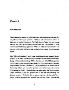
modules (MCMs) and the circuit boards found in many wireless consumer products. An example of a PCB assembly is shown in Figure 1.1. With the increase in operating frequency of devices in access of 100MHz and switching speed of digital devices within sub-nanoseconds (for example see Kobayashi et al 1992, Koga 1994), electromagnetic interference, stray parameters of components and unintentional radiation have become a major concern. This has been aggravated by the trend to pack as many components as possible into a unit area of the PCB. Such undesirable effects often undermine the integrity of electrical signal propagating within the PCB assembly and introduce noise, degrading the performance of the system.

Integrated circuits

Surface mount discrete component

Figure 1.1 – An example of printed circuit board assembly.

1

It has come to a stage that in almost every design of high-frequency electronic systems, the design is no longer confined to the schematic of the circuit. Selection of the package type, placement and orientation of components, the metallic traces, the dielectric material and other structures in the PCB assembly all affect the performance of the system. For microwave circuits, use of distributed elements like transmission line, resonator patch and periodic structures requires elements that are fabricated on the PCB itself. These elements have no lumped circuit counterparts in circuit analysis. In other words we no longer view the operation of an electronic circuit as just the interaction of currents and voltages flowing between the pins of the components. The electromagnetic fields surrounding the components and the system also determine how the system will function. This calls for a new design and analysis method that would consider the physical system in its entity, not by abstracting a physical system into a collection of circuit elements with component symbols and inter-connecting them with ideal wires. Traditionally analog/digital circuit design relies on the use of SPICE (Simulation Program with Integrated Circuit Emphasis) based computer software (Kielkowski 1998, Massobrio and Antognetti, 1993). This is a circuit-based approach, it started as a research project in University of California, Berkeley in the early 1970s. The source code for SPICE is eventually placed in the public domain (current version is SPICE3, written in the programming language C).

The algorithms used in SPICE based

simulation programs are robust, linear and nonlinear lumped components are supported and the algorithm can handle circuits with hundreds or even thousands of transistors. The SPICE algorithm is embedded into many commercial Electronic Design Automation (EDA) tools today (Kielkowski 1998). The circuit-based simulator can be extended to take into account the interaction of electromagnetic fields between components and metallic structures in the PCB assembly. This can be done where quasi-static assumption is valid with medium component and trace density on the PCB (Kung 1997, Scott 1994). Quasi-static implies that phasors for electric and magnetic fields in a.c. condition are very similar to the d.c. electromagnetic fields. For instance

2

the electromagnetic field interaction between two adjacent metallic structures can be represented using mutual inductance and capacitance between the conductors. For a collection of conductors one would obtain an inductance and capacitance matrix. This can be cast into a circuit definition in SPICE and solved using the SPICE simulation engine. By introducing single and coupled transmission line models into SPICE and using proper models, this approach can account for the effect of electromagnetic fields interaction up to operating frequency of 4GHz (This method is called Structural Approach in Kung (1997)). For very high frequency system where quasi-static no longer applies, this approach will not be accurate. Nor will it be efficient if the metallic structures in the PCB are tightly packed, then the equivalent circuit for the system will become extremely large. Obviously for very high frequency and very dense PCB assembly the field based approach is needed. This is called the full-wave approach (Naishadham 1993). In the full-wave approach the Maxwell’s equations for the system is considered without any simplification as in quasi-static approach. Numerical method is then applied to find the approximate electric (E) and magnetic (H) field components at various locations in the system. Once the approximate field components are obtained, equivalent current and voltage can be defined by: b

Vba = − ∫ E ⋅ dl

(1.1.1)

I = ∫ H ⋅ dl

(1.1.2)

a

C

In (1.1.2) C denotes a closed path encircling the conductor with electric current flowing within it, a and b denote two different points on the conducting structures of the model. Note that (1.1.1) and (1.1.2) are only accurate where quasi-static mode or quasi-TEM (Transverse Electric Magnetic) propagation mode is valid in the system (Collins 1993). For very high frequency system we usually do away with the notion of voltage and current, it is simply the interaction of the electric and magnetic fields in the system and the physics of each component that determines the outcome.

3

1.2 Numerical Method of Choice The wide variety of numerical techniques (see Itoh 1989) for electromagnetic field analysis can be categorized into two groups, e.g. differential and integral. All methods discretize the problem region and transform the field equations into a system of linear equations. Differential methods such as Finite Element Methods (FEM) (Itoh 1989) and Finite-Difference Time-Domain (FDTD) (Yee 1966) require discretization of the entire problem region.

Integral methods such as Method of Moments (MoMs)

(Harrington 1968) only require discretization over the conductor surface.

Another

popular method, the Transmission Line Matrix (TLM) method (Itoh 1989, Hoefer 1985), can be considered a differential method. All these methods invariably use the Maxwell’s equations in time-domain or time-harmonic forms. The time-domain and time-harmonic forms of Maxwell’s equations are included below as a reference. Time-domain Maxwell’s equations ∇ × E = − ∂∂t B


(1.2.2a)




∇ × H = J + ∂∂t D

(1.2.2b)

∇ ⋅ D = ρe

(1.2.2c)

∇⋅B =0

(1.2.2d)















Time-harmonic Maxwell’s equations ∇ × E = − jωµH





(1.2.3a)

∇ × H = J + jωεE

(1.2.3b)

ε∇ ⋅ E = ρ e

(1.2.3c)













(1.2.3d)

∇⋅H =0 

D = ε E and B = µ H 






(1.2.3e)




In (1.2.2a)-(1.2.2d) and (1.2.3a)-(1.2.3d), the magnetic charge density and the magnetic current density are ignored. Furthermore, all the vector variables in (1.2.3a)–

4

(1.2.3e) are complex phasors (note the non-italized font used to represent phasors). It must be emphasized that time-harmonic Maxwell’s equations are obtained from Fourier Transform. The field components in time-harmonic form are phasors, which represent the steady state sinusoidal fields at a particular frequency.

An inverse Fourier

Transform operation has to be performed to obtain the time-domain response. Timeharmonic Maxwell’s equations are not suitable for nonlinear system as harmonics are generated for every sinusoidal component at steady state. Moreover the concept of harmonics is not applicable during transient state. Method of Moment (MoM) and the Finite Element Method (FEM) usually employ time-harmonic Maxwell’s equations. As a result, these methods are largely confined to linear systems. The Finite-Difference Time-Domain (FDTD) and Transmission Line Matrix (TLM) methods are based on time-domain Maxwell’s equations. The E and H field components provided by FDTD and TLM methods are the transient fields, which are functions of time. Because of this, nonlinear elements and dielectric can be incorporated into both methods, and both methods are equally versatile (Paul et.al 1999). In the TLM method, the field problem is converted to a three-dimensional equivalent network problem of interconnecting transmission lines. For the FDTD method, approximate solution to the field problem is solved by applying finite-difference operators to the time-domain Maxwell’s equations directly without having to convert the problem into another form. The method-of-choice for this thesis is the Finite-Difference Time-Domain (FDTD) approach. This thesis uses the formulation initially proposed by Yee, which has come a long way since the landmark paper by K. S. Yee in 1966 (Yee 1966). The Yee’s algorithm, as it is usually called in the literature, is well known for its robustness and versatility. The method approximates the differentiation operators of the Maxwell equations with finite-difference operators in time and space. This method is suitable for finding the approximate electric and magnetic fields in a complex three-dimensional structure in the time domain. Many researchers have contributed immensely to extend the method to many areas of science and engineering (Taflove 1995, 1998). Initially the FDTD method is used for simulating electromagnetic waves scattering from object and

5

radar cross section measurement (Taflove 1975, Kunz and Lee, 1978, Umashankar and Taflove, 1982 ). In recent years there is a proliferation of focus in using the method to simulate microwave circuits and printed circuit board (Zhang and Mei 1988, Sheen et.al 1990, Sui et.al 1992, Toland and Houshmand 1993, Piket-May et.al 1994, Ciampolini et.al 1996, Kuo et.al 1997, Emili et.al 2000). Initially Zhang and Mei (1988) and Sheen et.al (1990) concentrate on modeling planar circuits using FDTD method. Later Sui et.al (1992) and Toland and Houshmand (1993) introduce the lumped-element FDTD approach. This enable the incorporation of ideal lumped elements such as resistor, capacitor, inductor and PN junction. Piket-May et.al (1994) refined the method further with the introduction of Eber-Molls transistor model and the resistive voltage source. All these components coincide with an electric field component in the model. Ciampolini et.al (1996) introduces a more realistic PN junction and transistor model taking into account junction capacitance. Furthermore adaptive time-step is used to prevent non-convergent of the nonlinear solution, particularly when there is rapid change in the voltage across the PN junction. In 1997, Kuo et.al presented a paper detailing a FDTD model with metal-semiconductor field effect transistor (MESFET). Recently Emili et.al (2000) introduces an extension of the lumped-element FDTD which enable PN junction, resistor, inductor and capacitor to be combined into a single component. Parallel to the development in including lumped circuit elements into FDTD formulation, another significant advance occurs with the development of frequency dependent FDTD method (Luebbers and Hunsberger, 1992).

This

development allows modeling of system with linearly dispersive dielectric media. Further developments by Gandhi et.al (1993) and Sullivan (1996) enable the inclusion of general dispersive media, where in addition to dispersive, the dielectric can also behave nonlinearly under intense field excitation. A detailed survey in this area can also be found in Chapter 9 of the book by Taflove (1995). 1.3 Scope of the Thesis The objective of this thesis is to come up with a systematic framework for modeling electromagnetic wave propagation in a printed circuit board (PCB) assembly and related

6

structures. The PCB assembly contains discrete components (both active and passive), integrated circuits, copper traces, sockets and connectors. Related structures imply this framework could be generalized to environments such as Monolithic Microwave Integrated Circuit (MMIC) and the semiconductor itself.

The author draws upon

previous contributions by past researchers and improves on a few key areas (notably lumped diode and transistor modeling) to enable the FDTD approach to effectively model a complete PCB assembly. Furthermore the questions of stability of the method, when applied to models containing nonlinear elements and discontinuity in the dielectric, has been answered, at least in the context of PCB modeling. The main contributions of this project are: •

Proposed a suitable method to include practical diode and bipolar junction transistor models into the FDTD framework. The proposed method is non-recursive, does not suffer from non-convergence problem and compatible with the industry standard SPICE models.

•

Developed and derived a rigorous stability theory for the FDTD framework based on nonlinear discrete dynamical system theory (Scheinerman 1996, Elaydi 2000). FDTD, being an iterative numerical method, is susceptible to divergence, where the solution of electric and magnetic fields blow up as time progresses. In a linear, nondispersive and homogeneous dielectric with no lumped elements, the cause of this divergence can be identified using Discrete Fourier Transform (DFT) (Oppenheim and Schafer 1989). Using DFT, it is shown that when certain condition, known as the Courant-Friedrich-Lewy (CFL) Stability Criterion is not fulfilled, there will be numerical wave components which increase with simulation time-step. The DFT method relies on superposition principle and assuming infinite region. Thus in a model with nonlinear lumped elements, finite computational domain and discontinuity in the dielectrics, the DFT method is not valid and the CFL Stability Criterion is at best a rule-of-thumb.

In this project, the FDTD framework is

recognized as a discrete dynamical system. Ideas from nonlinear stability theory in the theory of motions in mechanics (Merkin 1997, Khalil 1996, Elaydi 2000) are adapted to the FDTD framework and a new stability criterion is derived. This

7

criterion is applicable to both linear and nonlinear systems, with non-homogeneous dielectric and a few simple boundaries condition taken into account. Any FDTD model fulfilling the new stability criterion is shown to be stable without resorting to running lengthy computer simulation to verify its stability. •

Finally a self-contained software is developed, incorporating the graphical-userinterface (GUI) for user to construct a three-dimensional model, a FDTD simulation engine designed using object-oriented approach (written in ANSI compliant C++) and a simple graphing utility to view the electric and magnetic fields. From the electromagnetic field components, equivalent voltage and current can be derived, which is useful for microwave circuit design. The software runs on Windows platform. The simulation engine is developed in a systematic manner so that it can be extended in future to incorporate more features.

It is written in the C++

programming language and can be compiled to run on other operating systems such as LINUX and UNIX. A convenient and flexible notation for describing complex three-dimensional models is also introduced. This notation describes the model cube-by-cube, using lines of compact syntax. With this notation, many different types of model can be rapidly constructed without having to modify the declaration in the FDTD simulation engine.

The description of the model is stored in a

computer file, the FDTD simulation engine simply read the model file, set up necessary memory requirements in the computer and the simulation is ready to proceed. Since it is not possible to embody all the progresses and advancements of FDTD into the thesis, the printed circuit board (PCB) model considered is limited to the followings: •

The lumped components include resistor, capacitor, inductor, diode, bipolar junction transistor and resistive voltage source.

•

All conductors in the PCB are assumed to be perfect electric conductor.

8

•

Dielectric material is isotropic, non-dispersive and non-magnetic ( µ = µ o ). However the permittivity ε of the dielectric is allowed to vary as a function of location, field intensity and also time.

1.4 General Overview of the Contents The following is a brief account of the rest of the contents of this thesis. Chapter Two provides some fundamental concepts on the application of finite-difference method to partial differential equations. Concepts such as accuracy of the method, convergence and stability will be discussed in details. An important theorem in finite-difference method, the Lax Equivalence Theorem (Richtmyer and Morton, 1967) is also put forward in Chapter Two. This theorem is relevant to linear systems (i.e. when the partial differential equation describing the system is linear). Chapter Three introduces the Yee’s FDTD formulation.

Various notations such as the naming for field

components, the coordinate of the cubes etc. are standardized. In this chapter some issues of the FDTD method such as accuracy, numerical dispersion and stability will be discussed in detail. The definitions and theorems put forward in Chapter Two also apply to Yee’s FDTD formulation. In particular if the system is linear, then Lax Equivalence Theorem is also valid for the FDTD scheme for Maxwell’s equations. Furthermore, the notion of absorbing boundary condition will also be introduced. Chapter Four discusses various methods to incorporate linear and nonlinear lumped components into the FDTD framework such as resistor, voltage source, capacitor, inductor, diode and bipolar junction transistor. Chapter Five introduces the concept of constructing a complex threedimensional model of PCB using dielectric cubes and the FDTD simulation program. A syntax for describing the model is discussed.

High level overview of the FDTD

simulation engine, the process flow and the various data structures used in the software is provided.

At the end of Chapter Five, a few sample simulation examples are

presented to illustrate the effectiveness of the program. In Chapter Six, new stability theorems based on energy method are proposed. The inspiration of the energy method

9

is derived from similar stability theorems in nonlinear dynamical systems (Merkin 1997, Elaydi 2000). Here it is suggested that similar to the actual physical system, the FDTD model contains a numerical energy which is a function of all the field components. If the numerical energy is limited, then the field components will also be bounded, implying stability. The proofs of the theorems are shown in Appendix 3 to Appendix 6 and application of the theorems to establish stability of the PCB model is shown in the main text. In Chapter Seven, more simulation examples are provided. The simulation examples in Chapter Seven are substantiated by comparison with results from measurements or from commercial simulation package. An instability example is also demonstrated in Chapter Seven, to verify the ideas suggested in Chapter Six. Here it is shown that a bipolar junction transistor biased beyond its stable operating region causes the numerical energy of the system to increase dramatically. This results in the divergence of the electromagnetic field components. Finally Chapter Eight summarizes the work and provides a brief conclusion to the thesis.

10