Chapter 1 - Introduction to Statistics

CHAPTER

1

Introduction to Statistics LEARNING OBJECTIVES After reading this chapter, you should be able to:

1 Distinguish between descriptive and inferential statistics.

1.1

1.2 Statistics in Research 1.3

Scales of Measurement

1.4

Types of Data

1.5

Research in Focus: Types of Data and Scales of Measurement

1.6

SPSS in Focus: Entering and Defining Variables

2 Explain how samples and populations, as well as a sample statistic and population parameter, differ.

3 Describe three research methods commonly used in behavioral science.

4 State the four scales of measurement and provide an example for each.

5 Distinguish between qualitative and quantitative data. 6 Determine whether a value is discrete or continuous. 7 Enter data into SPSS by placing each group in separate columns and each group in a single column (coding is required).

Descriptive and Inferential Statistics

2

PART I: INTRODUCTION AND DESCRIPTIVE STATISTICS

1.1 DESCRIPTIVE AND INFERENTIAL STATISTICS Why should you study statistics? The topic can be intimidating, and rarely does anyone tell you, “Oh, that’s an easy course . . . take statistics!” Statistics is a branch of mathematics used to summarize, analyze, and interpret what we observe—to make sense or meaning of our observations. A family counselor may use statistics to describe patient behavior and the effectiveness of a treatment program. A social psychologist may use statistics to summarize peer pressure among teenagers and interpret the causes. A college professor may give students a survey to summarize and interpret how much they like (or dislike) the course. In each case, the counselor, psychologist, and professor make use of statistics to do their job. The reason it is important to study statistics can be described by the words of Mark Twain: “There are lies, damned lies and statistics.” He meant that statistics can be deceiving—and so can interpreting them. Statistics are all around you—from your college grade point average (GPA) to a Newsweek poll predicting which political candidate is likely to win an election. In each case, statistics are used to inform you. The challenge as you move into your careers is to be able to identify statistics and to interpret what they mean. Statistics are part of your everyday life, and they are subject to interpretation. The interpreter, of course, is YOU.

DEFINITION

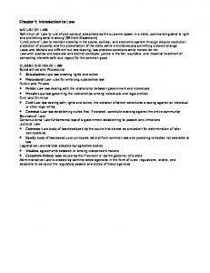
Statistics is a branch of mathematics used to summarize, analyze, and interpret a group of numbers or observations. We begin by introducing two general types of statistics: •• Descriptive statistics: statistics that summarize observations. •• Inferential statistics: statistics used to interpret the meaning of descriptive statistics. This book describes how to apply and interpret both types of statistics in science and in practice to make you a more informed interpreter of the statistical information you encounter inside and outside of the classroom. Figure 1.1 is a schematic diagram of the chapter organization of this book, showing which chapters focus on descriptive statistics and which focus on inferential statistics.

DESCRIPTIVE STATISTICS Researchers can measure many behavioral variables, such as love, anxiety, memory, and thought. Often, hundreds or thousands of measurements are made, and procedures were developed to organize, summarize, and make sense of these measures. These procedures, referred to as descriptive statistics, are specifically used to describe or summarize numeric observations, referred to as data. To illustrate, suppose we want to study anxiety among college students. We could describe anxiety, then, as a state or feeling of worry and nervousness. This certainly describes anxiety, but not numerically (or in a way that allows us to measure anxiety). Instead, we could state that anxiety is the number of times students fidget during a class presentation. Now anxiety is defined as a number. We may observe 50, 100, or 1,000 students give a class presentation and record the number of times each

C H APT ER 1 : I N T RO D U C T I O N T O S TAT I S T I C S

3

Transition from descriptive to inferential statistics (Chapters 6-7) Inferential Statistics (Chapters 8-18)

Descriptive Statistics (Chapters 2-5)

FIGURE 1.1

Statistics

A general overview of this book. This book begins with an introduction to descriptive statistics (Chapters 2–5) and then uses descriptive statistics to transition (Chapters 6–7) to a discussion of inferential statistics (Chapters 8–18).

student fidgeted. Presenting a spreadsheet with the number for each individual student is not very clear. For this reason, researchers use descriptive statistics to summarize sets of individual measurements so they can be clearly presented and interpreted. Descriptive statistics are procedures used to summarize, organize, and make sense of a set of scores or observations. Descriptive statistics are typically presented graphically, in tabular form (in tables), or as summary statistics (single values).

DEFINITION

Data (plural) are measurements or observations that are typically numeric. A datum (singular) is a single measurement or observation, usually referred to as a score or raw score. Data are generally presented in summary. Typically, this means that data are presented graphically, in tabular form (in tables), or as summary statistics (e.g., an average). For example, the number of times each individual fidgeted is not all that meaningful, whereas the average (mean), middle (median), or most common (mode) number of times among all individuals is more meaningful. Tables and graphs serve a similar purpose to summarize large and small sets of data. Most often, researchers collect data from a portion of individuals in a group of interest. For example, the 50, 100, or 1,000 students in the anxiety example would not constitute all students in college. Hence, these researchers collected anxiety data from some students, not all. So researchers require statistical procedures that allow them to infer what the effects of anxiety are among all students of interest using only the portion of data they measured.

NOTE: Descriptive statistics summarize data to make sense or meaning of a list of numeric values.

4


INFERENTIAL STATISTICS The problem described in the last paragraph is that most scientists have limited access to the phenomena they study, especially behavioral phenomena. As a result, researchers use procedures that allow them to interpret or infer the meaning of data. These procedures are called inferential statistics.

DEFINITION

Inferential statistics are procedures used that allow researchers to infer or generalize observations made with samples to the larger population from which they were selected. To illustrate, let’s continue with the college student anxiety example. All students enrolled in college would constitute the population. This is the group that researchers want to learn more about. Specifically, they want to learn more about characteristics in this population, called population parameters. The characteristics of interest are typically some descriptive statistic. In the anxiety example, the characteristic of interest is anxiety, specifically measured as the number of times students fidget during a class presentation. Unfortunately, in behavioral research, scientists rarely know what these population parameters are since they rarely have access to an entire population. They simply do not have the time, money, or other resources to even consider studying all students enrolled in college.

DEFINITION

A population is defined as the set of all individuals, items, or data of interest. This is the group about which scientists will generalize. A characteristic (usually numeric) that describes a population is referred to as a population parameter.

NOTE: Inferential statistics are used to help the researcher infer how well statistics in a sample reflect parameters in a population.

DEFINITION

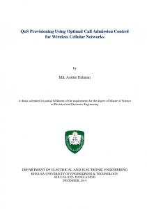
The alternative is to select a portion or sample of individuals in the population. Selecting a sample is more practical, and most scientific research you read comes from samples and not populations. Going back to our example, this means that selecting a portion of students from the larger population of all students enrolled in college would constitute a sample. A characteristic that describes a sample is called a sample statistic—this is similar to a parameter, except it describes characteristics in a sample and not a population. Inferential statistics use the characteristics in a sample to infer what the unknown parameters are in a given population. In this way, as shown in Figure 1.2, a sample is selected from a population to learn more about the characteristics in the population of interest. A sample is defined as a set of selected individuals, items, or data taken from a population of interest. A characteristic (usually numeric) that describes a sample is referred to as a sample statistic.


5

Population: All students enrolled in college.

Sample: 50 students 100 students 1,000 students

Draw conclusions about anxiety levels for the entire population of students (not just among those in each sample).

Observe the number of times each student fidgets during a class presentation in each sample.

MAKING SENSE: Populations and Samples A population is identified as any group of interest, whether that group is all students worldwide or all students in a professor’s class. Think of any group you are interested in. Maybe you want to understand why college students join fraternities and sororities. So students who join fraternities and sororities is the group you’re interested in. Hence, this group is now a population of interest, to you anyways. You identified a population of interest just as researchers identify populations they are interested in. Remember that researchers collect samples only because they do not have access to all individuals in a population. Imagine having to identify every person who has fallen in love, experienced anxiety, been attracted to someone else, suffered with depression, or taken a college exam. It’s ridiculous to consider that we can identify all individuals in such populations. So researchers use data gathered from samples (a portion of individuals from the population) to make inferences concerning a population. To make sense of this, say you want to get an idea of how people in general feel about a new pair of shoes you just bought. To find out, you put your new shoes on and ask 20 people at random throughout the day whether or not they like the shoes. Now, do you really care about the opinion of only those 20 people you asked? Not really—you actually care more about the opinion of people in general. In other words, you only asked the 20 people (your sample) to get an idea of the opinions of people in general (the population of interest). Sampling from populations follows a similar logic.

FIGURE 1.2 Samples and populations. In this example, levels of anxiety were measured in a sample of 50, 100, or 1,000 college students. Researchers will observe anxiety in each sample. Then they will use inferential statistics to generalize their observations in each sample to the larger population, from which each sample was selected.

6


E X A M PL E 1.1

On the basis of the following example, we will identify the population, sample, population parameter, and sample statistic: Suppose you read an article in the local college newspaper citing that the average college student plays 2 hours of video games per week. To test whether this is true for your school, you randomly approach 20 fellow students and ask them how long (in hours) they play video games per week. You find that the average student, among those you asked, plays video games for 1 hour per week. Distinguish the population from the sample. In this example, all college students at your school constitute the population of interest, and the 20 students you approached is the sample that was selected from this population of interest. Since it is purported that the average college student plays 2 hours of video games per week, this is the population parameter (2 hours). The average number of hours playing video games in the sample is the sample statistic (1 hour).

LE A R N I N G C H EC K 1

1. _____________ are techniques used to summarize or describe numeric data. 2. __________ describe(s) how a population is characterized, whereas _____________ describe(s) the characteristics of samples. a. Statistics; parameters b. Parameters; statistics c. Descriptive; inferential d. Inferential; descriptive 3. A psychologist wants to study a small population of 40 students in a local private school. If the researcher was interested in selecting the entire population of students for this study, then how many students must the psychologist include? a. None, since it is not possible to study an entire population in this case. b. At least half, since this would constitute the majority of the population. c. All 40 students, since all students constitute the population. 4. True or false: Inferential statistics are used to help the researcher infer whether observations made with samples are reflective of the population. Answers: 1. Descriptive statistics; 2. B; 3. C; 4. True.

1.2 STATISTICS IN RESEARCH This book will describe many ways of measuring and interpreting data. Yet, simply collecting data does not make you a scientist. To engage in science, you must follow specific procedures for collecting data. Think of this as playing a game. Without the rules and procedures for playing, the game itself would be lost. The same is true in science; without the rules and procedures for collecting data, the ability to draw scientific conclusions would be lost. Ultimately, statistics are used in the context of science, and so it is necessary to introduce you to the basic procedures of scientific inquiry.


To illustrate the basic premise of engaging in science, suppose you come across the following problem first noted by the famous psychologist Edward Thorndike in 1898: Dogs get lost hundreds of times and no one ever notices it or sends an account of it to a scientific magazine, but let one find his way from Brooklyn to Yonkers and the fact immediately becomes a circulating anecdote. Thousands of cats on thousands of occasions sit helplessly yowling, and no one takes thought of it or writes to his friend, the professor; but let one cat claw at the knob of a door supposedly as a signal to be let out, and straightway this cat becomes the representative of the cat-mind in all books. . . . In short, the anecdotes give really . . . supernormal psychology of animals. (pp. 4–5) Science is the study of phenomena, such as behavior, through strict observation, evaluation, interpretation, and theoretical explanation.

DEFINITION

Here the problem was to determine the animal mind. Edward Thorndike posed the question of whether animals were truly smart, based on the many observations he made. This is where the scientific process typically begins—with a question. To answer questions in a scientific manner, researchers need more than just statistics; they need a set of strict procedures for making the observations and measurements. In this section, we introduce three research methods commonly used in behavioral research: experimental, quasi-experimental, and correlational methods. Each research method involves examining the relationship between variables. Each method is introduced here since we will apply these methods throughout the book.

EXPERIMENTAL METHOD Any study that demonstrates cause is called an experiment. To demonstrate cause, though, an experiment must follow strict procedures to ensure that the possibility of all other possible causes have been minimized or eliminated. So researchers must control the conditions under which observations are made to isolate cause-andeffect relationships between variables. Figure 1.3 shows the steps in a typical experiment based on a sample taken from a population. We will work through this example to describe the basic structure of an experiment. To conduct an experiment, a researcher must specifically control the conditions under which observations are made to isolate cause-and-effect relationships between variables. Three requirements must be satisfied for a study to be regarded as an experiment: randomization, manipulation, and comparison. The experiment illustrated in Figure 1.3 was designed to determine the effect of distraction on student test scores. A sample of students was selected from a population of all undergraduates. In one group, the professor sat quietly while students took the exam (low-distraction group); in the other, the professor rattled papers, tapped her foot, and made other sounds during the exam (high-distraction group). Exam scores in both groups were measured and compared. For this study to be called an experiment, researchers must satisfy three requirements. These requirements are regarded as the necessary steps to ensure enough

DEFINITION

7

8


Population

FIGURE 1.3 The basic structure of an experiment that meets each requirement for demonstrating cause-and-effect: randomization, manipulation, and comparison. In this example, a random sample of students was selected from a population of all undergraduates to study the effects of distraction on exam performance. To qualify as an experiment, (1) students were randomly assigned to experience a low- or highdistraction condition while taking an exam (randomization), (2) the researcher created each level of distraction (manipulation), and (3) a comparison group was included where distraction was minimal or absent (comparison).

Sample Manipulate one variable— randomly assign participants to each level of the manipulated variable. Example: Randomly assign participants to two levels of distraction.

Low-distraction condition: A professor sits quietly at a desk while students take an exam.

High-distraction condition: A professor makes loud sounds (paper ruffling, foot tapping) at a desk while students take an exam.

Measure grades on exam (0–100 points).

Measure grades on exam (0–100 points).

Measure a second variable— the same variable is measured in each condition, and the difference between groups is compared. Example: Measure exam performance (or grades) in each condition.

control to allow researchers to draw cause-and-effect conclusions. These requirements are the following: 1. Randomization (of assigning participants to conditions) 2. Manipulation (of variables that operate in an experiment) 3. Comparison (or a control group) To meet the requirement of randomization, researchers must use random assignment (Requirement 1) to assign participants to groups. To do this, a researcher must be able to manipulate the levels of an independent variable (IV) (Requirement 2) to create the groups. Referring back to the test distraction example shown in Figure 1.3, the independent variable was distraction. The researchers first manipulated the levels of this variable (low, high), meaning that they created the conditions. They then assigned each student at random to experience one of the levels of distraction.

DEFINITION

Random assignment is a random procedure used to ensure that participants in a study have an equal chance of being assigned to a particular group or condition. An independent variable (IV) is the variable that is manipulated in an experiment. This variable remains unchanged (or “independent”) between conditions being observed in an experiment. It is the “presumed cause.” The specific conditions of an IV are referred to as the levels of the IV. Random assignment and manipulation ensure that characteristics of participants in each group (such as their age, intelligence level, or study habits) vary entirely by chance. Since participant characteristics between groups now occur at


random, we can assume that these characteristics are about the same between groups. This makes it more likely that any differences observed between groups were caused by the manipulation (low vs. high levels of distraction) and not participant characteristics. Notice also that there are two groups in the experiment shown in Figure 1.3. So tests scores for students experiencing high levels of distraction were compared to those experiencing low levels of distraction. By comparing test scores between groups, we can determine whether high levels of distraction caused lower scores (compared to scores in the low-distraction group). This satisfies the requirement of comparison (Requirement 3), which requires that at least two groups be observed in an experiment. This allows scores in one group to be compared to those in at least one other group. In this example, test scores were measured in each group. The measured variable in an experiment is referred to as the dependent variable (DV). Dependent variables can often be measured in many ways, and therefore require an operational definition. This is where a dependent variable is defined in terms of how it will be measured. For example, here we operationally defined exam performance as a score between 0 and 100 on a test. So to summarize the experiment in Figure 1.3, levels of distraction (IV) were presumed to cause an effect or difference in exam grades (DV) between groups. This is an experiment since the researchers satisfied the requirements of randomization, manipulation, and comparison, thereby allowing them to draw cause-and-effect conclusions. The dependent variable (DV) is the variable that is believed to change in the presence of the independent variable. It is the “presumed effect.”

9

NOTE: An experiment is one where researchers satisfy three requirements to ensure enough control to allow researchers to draw cause-and-effect conclusions. These are randomization, manipulation, and comparison.

DEFINITION

An operational definition is a description of some observable event in terms of the specific process or manner by which it was observed or measured.

QUASI-EXPERIMENTAL METHOD A study that lacks randomization, manipulation, or comparison is called a quasi-experiment. This most often occurs in one of two ways: 1. The study includes a quasi-independent variable. 2. The study lacks a comparison group. In a typical quasi-experiment, the variables being studied can’t be manipulated, which makes random assignment impossible. This occurs when variables are preexisting or inherent to the participants themselves. These types of variables are called quasi-independent variables. Figure 1.4 shows an example of a quasi-experiment that measured differences in multitasking ability by gender. Since the levels of gender (male, female) can’t be randomly assigned (it is a quasi-independent variable), this study is regarded as a quasi-experiment. A quasi-independent variable is a variable whose levels are not randomly assigned to participants (nonrandom). This variable differentiates the groups or conditions being compared in a quasi-experiment.

DEFINITION NOTE: A quasi-experiment is

A study is also regarded as a quasi-experiment when only one group is observed. Since only one group is observed, there is no comparison group. So differences between two levels of an independent variable can’t be compared. In this

a study that (1) includes a quasi-independent variable or (2) lacks a comparison group.

10


Gender is not randomly assigned. Men are assigned to the male condition; women to the female condition.

A sample of men and women is selected from a population.

FIGURE 1.4 The basic structure of a quasiexperiment. In this example, researchers measured differences in multitasking behavior by gender. The grouping variable (gender) is preexisting. That is, participants were already male or female prior to the study. For this reason, researchers can’t manipulate the variable or randomly assign participants to each level of gender, so this study is regarded as a quasi-experiment.

Male condition: Men are asked to complete as many tasks as possible in 5 minutes.

Female condition: Women are asked to complete as many tasks as possible in 5 minutes.

Dependent measure: The number of tasks completed is recorded.

Dependent measure: The number of tasks completed is recorded.

way, failing to satisfy any of the three requirements for an experiment (randomization, manipulation, or comparison) makes the study a quasi-experiment.

CORRELATIONAL METHOD

NOTE: The correlational method involves measuring the relationship between pairs of scores.

E X A M PL E 1. 2

Another method for examining the relationship between variables is to measure pairs of scores for each individual. This method can determine whether a relationship exists between variables, but it lacks the appropriate control needed to demonstrate cause and effect. To illustrate, suppose you test for a relationship between time spent using a computer and exercising per week. The data for such a study appear in tabular form and plotted as a graph in Figure 1.5. Using the correlational method, we can examine the extent to which two variables change in a related fashion. In the example shown in Figure 1.5, as computer use increases, time spent exercising decreases. This pattern suggests that computer use and time spent exercising are related. Notice that no variable is manipulated to create different conditions or groups to which participants can be randomly assigned. Instead, two variables are measured for each participant, and the extent to which those variables are related is measured. This book will describe many statistical procedures used to analyze data using the correlational method (Chapters 15–17) and the experimental and quasi-experimental methods (Chapters 9–14, 17–18). A researcher conducts the following study: Participants are presented with a list of words written on a white background on a PowerPoint slide. In one group, the words are written in red (Group Color); in a second group, the words are written in black (Group Black). Participants are allowed to study the words for 1 minute. After that time, the slide is removed and participants are allowed 1 minute to write down as many words as they can recall. The number of words correctly recalled will be recorded for each group. Explain how this study can be an experiment.


(a)

(b)

Participant

Computer use (Hours per week)

Exercise (Minutes per week)

A

3

80

B

2

83

C

0

96

D

10

60

E

8

78

F

12

46

11

120 FIGURE 1.5

Exercise (Minutes per week)

100 80 60 40 20 0 0

2

4

6

8

10

12

14

Computer Use (Hours per week)

To create an experiment, we must satisfy the three requirements for demonstrating cause and effect: randomization, manipulation, and comparison. To satisfy each requirement, the researcher can 1. Randomly assign participants to experience one of the conditions. This ensures that some participants read colored words and others read black words entirely by chance. 2. Create the two conditions. The researcher could write 20 words on a PowerPoint slide. On one slide, the words are written in red; on the second slide, the same words are written in black. 3. Include a comparison group. In this case, the number of colored words correctly recalled will be compared to the number of black words correctly recalled, so this study has a comparison group. Remember that each requirement is necessary to demonstrate that the levels of an independent variable are causing changes in the value of a dependent variable. If any one of these requirements is not satisfied, then the study is not an experiment.

An example of the correlational method. In this example, researchers measured the amount of time students spent using the computer and exercising each week. (A) The table shows two sets of scores for each participant. (B) The graph shows the pattern of the relationship between these scores. From the data, we can see that the two variables (computer use and exercise) change in a related fashion. That is, as computer use increases, time spent exercising decreases.

12



1. ____________ is the study of phenomena through strict observation, evaluation, interpretation, and theoretical explanation. 2. State whether each of the following describes an experiment, quasi-experiment, or correlational method. a. A researcher tests whether dosage level of some drug (low, high) causes significant differences in health. b. A researcher tests whether political affiliation (Republican, Democrat) is associated with different attitudes toward morality. c. A researcher measures the relationship between income and life satisfaction. 3. True or false: An experiment is the only method that can demonstrate causeand-effect relationships between variables. Answers: 1. Science; 2. A. Experiment. B. Quasi-experiment. C. Correlational method; 3. True.

1.3 SCALES OF MEASUREMENT Many statistical tests introduced in this book will require that variables in a study be measured on a certain scale of measurement. In the early 1940s, Harvard psychologist S. S. Stevens coined the terms nominal, ordinal, interval, and ratio to classify the scales of measurement (Stevens, 1946). Scales of measurement are rules that describe the properties of numbers. These rules imply that a number is not just a number in science. Instead, the extent to which a number is informative depends on how it was used or measured. In this section, we discuss the extent to which data are informative. In all, scales of measurement are characterized by three properties: order, differences, and ratios. Each property can be described by answering the following questions: 1. Order: Does a larger number indicate a greater value than a smaller number? 2. Differences: Does subtracting two numbers represent some meaningful value? 3. Ratio: Does dividing (or taking the ratio of) two numbers represent some meaningful value?

DEFINITION

Scales of measurement refer to how the properties of numbers can change with different uses. Table 1.1 summarizes the answers to the questions for each scale of measurement. You can think of each scale as a gradient of the informativeness of data. In this section, we begin with the least informative scale (nominal) and finish with the most informative scale (ratio).

NOMINAL SCALES Numbers on a nominal scale identify something or someone; they provide no additional information. Common examples of nominal numbers include ZIP codes,


13

TABLE 1.1 Scales of measurement. Different scales of measurement and the information they provide concerning the order, difference, and ratio of numbers.

Scale of Measurement

Property

Nominal

Ordinal

Interval

Ratio

Order

No

Yes

Yes

Yes

Difference

No

No

Yes

Yes

Ratio

No

No

No

Yes

license plate numbers, credit card numbers, country codes, telephone numbers, and Social Security numbers. These numbers simply identify locations, vehicles, or individuals and nothing more. One credit card number, for example, is not greater than another; it is simply different. Nominal scales are measurements where a number is assigned to represent something or someone. In science, nominal variables are typically categorical variables that have been coded—converted to numeric values. Examples of nominal variables include a person’s race, gender, nationality, sexual orientation, hair and eye color, season of birth, marital status, or other demographic or personal information. A researcher may code men as 1 and women as 2. They may code the seasons of birth as 1, 2, 3, and 4 for spring, summer, fall, and winter, respectively. These numbers are used to identify gender or the seasons and nothing more. We often code words with numeric values when entering them into statistical programs such as SPSS. Coding is largely done because it is often easier to compute data using statistical programs, such as SPSS, when data are entered as numbers, not words. Coding refers to the procedure of converting a nominal value to a numeric value.

DEFINITION NOTE: Nominal values represent something or someone. They often reflect coded data in behavioral science.

DEFINITION

ORDINAL SCALES An ordinal scale of measurement is one that conveys order alone. This scale indicates that some value is greater or less than another value. Examples of ordinal scales include finishing order in a competition, education level, and rankings. These scales only indicate that one value is greater or less than another, so differences between ranks do not have meaning. Consider, for example, the U.S. News & World Report rankings for the top psychology graduate school programs in the United States. Table 1.2 shows the rank, college, and actual score for the top 25 programs, including ties, in 2009. Based on ranks alone, can we say that the difference between the psychology graduate programs ranked 1 and 11 is the same as the difference between those ranked 13 and 23? In both cases, 10 ranks separate

NOTE: Ordinal values convey order alone.

14


TABLE 1.2 Ordinal scale. A list of the top 25 ranked psychology graduate school programs in 2009, including ties (left column), and the actual points used to determine their rank (right column). The U.S. News & World Report published these rankings.

Rank

College Name

Actual Score

1

Stanford University

4.7

1

University of California, Berkeley

4.7

3

Harvard University

4.6

3

University of California, Los Angeles

4.6

3

University of Michigan, Ann Arbor

4.6

3

Yale University

4.6

7

University of Illinois, Urbana-Champaign

4.5

8

Princeton University

4.4

8

University of Minnesota, Twin Cities

4.4

8

University of Wisconsin, Madison

4.4

11

Massachusetts Institute of Technology

4.3

11

University of Pennsylvania

4.3

13

University of North Carolina, Chapel Hill

4.2

13

University of Texas, Austin

4.2

13

University of Washington

4.2

13

Washington University in St. Louis

4.2

17

Carnegie Mellon University

4.1

17

Columbia University

4.1

17

Cornell University

4.1

17

Northwestern University

4.1

17

Ohio State University

4.1

17

University of California, San Diego

4.1

23

Duke University

4.0

23

Indiana University, Bloomington

4.0

23

John Hopkins University

4.0

the schools. Yet, if you look at the actual scores for determining rank, you find that the difference between ranks 1 and 11 is 0.4 points, whereas the difference between ranks 13 and 23 is 0.2 points. So the difference in points is not the same. Ranks alone don’t convey this difference. They simply indicate that one rank is greater or less than another rank.

DEFINITION

Ordinal scales are measurements where values convey order or rank alone.


15

INTERVAL SCALES An interval scale measurement, on the other hand, can be understood readily by two defining principles: equidistant scales and no true zero. A common example for this in behavioral science is the rating scale. Rating scales are taught here as an interval scale since most researchers report these as interval data in published research. This type of scale is a numeric response scale used to indicate a participant’s level of agreement or opinion with some statement. An example of a rating scale is given in Figure 1.6. Here we will look at each defining principle. Interval scales are measurements where the values have no true zero and the distance between each value is equidistant.

DEFINITION

An equidistant scale is a scale distributed in units that are equidistant from one another. Many behavioral scientists assume that scores on a rating scale are distributed in equal intervals. For example, if you are asked to rate your satisfaction with a spouse or job on a 7-point scale from 1 (completely unsatisfied) to 7 (completely satisfied), like in the scale shown in Figure 1.6, then you are using an interval scale. Since the distance between each point (1 to 7) is assumed to be the same or equal, it is appropriate to compute differences between scores on this scale. So a statement such as, “The difference in job satisfaction among men and women was 2 points,” is appropriate with interval scale measurements. Equidistant scales are those values whose intervals are distributed in equal units. However, an interval scale does not have a true zero. A common example of a scale without a true zero is temperature. A temperature equal to zero for most measures of temperature does not mean that there is no temperature; it is just an arbitrary zero point. Values on a rating scale also have no true zero. In the example shown in Figure 1.6, a 1 was used to indicate no satisfaction, not 0. Each value (including 0) is arbitrary. That is, we could use any number to represent none of something. Measurements of latitude and longitude also fit this criterion. The implication is that without a true zero, there is no value to indicate the absence of the phenomenon you are observing (so a zero proportion is not meaningful). For this reason, stating a ratio such as, “Satisfaction ratings were three times greater among men compared to women,” is not appropriate with interval scale measurements. A true zero describes values where the value 0 truly indicates nothing. Values on an interval scale do not have a true zero.

DEFINITION NOTE: Interval values have equidistant scales but no true zero.

DEFINITION

Satisfaction Ratings 1 2 3 4 5 6 7 Completely Unsatisfied

Completely Satisfied

FIGURE 1.6 An example of a 7-point rating scale for satisfaction used for scientific investigation.


NOTE: Ratio values have equidistant scales and a true zero. This scale of measurement does not limit the conclusions researchers can state.

DEFINITION

RATIO SCALES Ratio scales are similar to interval scales in that scores are distributed in equal units. Yet, unlike interval scales, a distribution of scores on a ratio scale has a true zero. This is an ideal scale in behavioral research because any mathematical operation can be performed on the values that are measured. Common examples of ratio scales include counts and measures of length, height, weight, and time. For scores on a ratio scale, order is informative. For example, a person who is 30 years old is older than another who is 20. Differences are also informative. For example, the difference between 70 and 60 seconds is the same as the difference between 30 and 20 seconds (the difference is 10 seconds). Ratios are also informative on this scale because a true zero is defined—it truly means nothing. Hence, it is meaningful to state that 60 pounds is twice as heavy as 30 pounds. Ratio scales are measurements where a set of values has a true zero and are equidistant. In science, researchers often go out of their way to measure variables on a ratio scale. For example, if they want to measure eating, they may choose to measure the amount of time between meals or the amount of food consumed (in ounces). If they measure memory, they may choose to measure the amount of time it takes to memorize some list or the number of errors made. If they measure depression, they may choose to measure the dosage (in milligrams) that produces the most beneficial treatment or the number of symptoms reported. In each case, the behaviors were measured using values on a ratio scale, thereby allowing researchers to draw conclusions in terms of order, differences, and ratios—there are no restrictions with ratio scale variables.


1. The ____________ refer to how the properties of numbers can change with different uses. 2. In 2010, Fortune 500 magazine ranked Apple as the most admired company in the world. This ranking is on a(n) ____________ scale of measurement. 3. What are two characteristics of rating scales that allow some researchers to use these values on an interval scale of measurement? a. Values on an interval scale have order and differences. b. Values on an interval scale have differences and a true zero. c. Values on an interval scale are equidistant and have a true zero. d. Values on an interval scale are equidistant and do not have a true zero. 4. Which of the following is not an example of a ratio scale variable? a. Age (in days) b. Speed (in seconds) c. Height (in inches) d. Movie ratings (1 to 4 stars) Answers: 1. Scales of measurement; 2. Ordinal; 3. D; 4. D.

16


17

TYPES OF DATA 1.4

The scales of measurement reflect the informativeness of data. With nominal scales, researchers can conclude little; with ratio scales, researchers can conclude just about anything in terms of order, differences, and ratios. Researchers also distinguish between the types of data they measure. The types of data researchers measure fall into two categories: (1) continuous or discrete and (2) quantitative or qualitative. Each category is discussed in this section. Many examples we use for these types of data are given in Table 1.3.

CONTINUOUS AND DISCRETE VARIABLES Variables can be categorized as continuous or discrete. A continuous variable is measured along a continuum. So continuous variables are measured at any place beyond the decimal point. Consider, for example, that Olympic sprinters are timed to the nearest hundredths place (in seconds), but if the Olympic judges wanted to clock them to the nearest millionths place, they could. A continuous variable is measured along a continuum at any place beyond the decimal point. Continuous variables can be measured in whole units or fractional units.

NOTE: Continuous variables are measured along a continuum, whereas discrete variables are measured in whole units or categories.

DEFINITION

A discrete variable, on the other hand, is measured in whole units or categories. So discrete variables are not measured along a continuum. For example, the number of brothers and sisters you have and your family’s socioeconomic class (working class, middle class, upper class) are examples of discrete variables. Refer to Table 1.3 for more examples of continuous and discrete variables. A discrete variable is measured in whole units or categories that are not distributed along a continuum.

DEFINITION

QUANTITATIVE AND QUALITATIVE VARIABLES Variables can be categorized as quantitative or qualitative. A quantitative variable varies by amount. The variables are measured in numeric units, and so both continuous and discrete variables can be quantitative. For example, we can measure food intake in calories (a continuous variable) or we can count the number of pieces of food consumed (a discrete variable). In both cases, the variables are measured by amount (in numeric units). A quantitative variable varies by amount. This variable is measured numerically and is often collected by measuring or counting.

DEFINITION

A qualitative variable, on the other hand, varies by class. The variables are often labels for the behaviors we observe—so only discrete variables can fall into this category. For example, socioeconomic class (working class, middle class, upper class) is discrete and qualitative; so are many mental disorders such as depression (unipolar, bipolar) or drug use (none, experimental, abusive). Refer to Table 1.3 for more examples of quantitative and qualitative variables. A qualitative variable varies by class. This variable is often represented as a label and describes nonnumeric aspects of phenomena.

DEFINITION

18


TABLE 1.3 A list of 20 variables showing how they fit into the three categories that describe them.

Variables

Continuous vs. Discrete

Qualitative vs. Quantitative


Gender (male, female)

Discrete

Qualitative

Nominal

Seasons (spring, summer, fall, winter)

Discrete

Qualitative

Nominal

Number of dreams recalled

Discrete

Quantitative

Ratio

Number of errors

Discrete

Quantitative

Ratio

Duration of drug abuse (in years)

Continuous

Quantitative

Ratio

Ranking of favorite foods

Discrete

Quantitative

Ordinal

Ratings of satisfaction (1 to 7)

Discrete

Quantitative

Interval

Body type (slim, average, heavy)

Discrete

Qualitative

Nominal

Score (from 0 to 100%) on an exam

Continuous

Quantitative

Ratio

Number of students in your class

Discrete

Quantitative

Ratio

Temperature (degrees Fahrenheit)

Continuous

Quantitative

Interval

Time (in seconds) to memorize a list

Continuous

Quantitative

Ratio

The size of a reward (in grams)

Continuous

Quantitative

Ratio

Position standing in line

Discrete

Quantitative

Ordinal

Political Affiliation (Republican, Democrat)

Discrete

Qualitative

Nominal

Type of distraction (auditory, visual)

Discrete

Qualitative

Nominal

A letter grade (A, B, C, D, F)

Discrete

Qualitative

Ordinal

Weight (in pounds) of an infant

Continuous

Quantitative

Ratio

A college students’ SAT score

Discrete

Quantitative

Interval

Number of lever presses per minute

Discrete

Quantitative

Ratio

E X A M PL E 1. 3

For each of the following examples, we will (1) name the variable being measured, (2) state whether the variable is continuous or discrete, and (3) state whether the variable is quantitative or qualitative. a. A researcher records the month of birth among patients with schizophrenia. The month of birth (the variable) is discrete and qualitative. b. A professor records the number of students absent during a final exam. The number of absent students (the variable) is discrete and quantitative. c. A researcher asks children to choose which type of cereal they prefer (one with a toy inside or one without). He records the choice of cereal for each child. The choice of cereal (the variable) is discrete and qualitative. d. A therapist measures the time (in hours) that clients continue a recommended program of counseling. The time in hours (the variable) is continuous and quantitative.


1. True or false: The types of data researchers measure fall into two categories: (1) continuous or discrete and (2) quantitative or qualitative.

19


2. State whether each of the following are continuous or discrete. a. Delay (in seconds) it takes drivers to make a left-hand turn when a light turns green b. The number of questions that participants ask during a research study c. Type of drug use (none, infrequent, moderate, or frequent) d. Season of birth (spring, summer, fall, or winter) 3. State whether the variables listed in Question 2 are quantitative or qualitative. 4. True or false: Qualitative variables can be continuous or discrete. 5. A researcher is interested in the effects of stuttering on social behavior with children. He records the number of peers a child speaks to during a typical school day. In this example, would the data be qualitative or quantitative? C. Qualitative. D. Qualitative; 4. False; 5. Quantitative. Answers: 1. True; 2. A. Continuous. B. Discrete. C. Discrete. D. Discrete; 3. A. Quantitative. B. Quantitative.

RESEARCH IN FOCUS: TYPES OF DATA AND SCALES OF MEASUREMENT 1.5

While qualitative variables are often measured in behavioral research, this book will focus largely on the latter. The reason is twofold: (1) Quantitative measures are more common in behavioral research, and (2) most statistical tests taught in this book are adapted for quantitative measures. Indeed, many researchers who measure qualitative variables will also measure those that are quantitative in the same study. For example, Jones and colleagues (2010) explored the costs and benefits of social networking among college students. The researchers used a qualitative method to interview each student in their sample. In the interview, students could respond openly to questions asked during the interview. These researchers then summarized responses into categories related to learning, studying, and social life. For example, the following student response was categorized as an example of independent learning experience for employability: “I think it [social software] can be beneficial . . . in the real working environment” (p. 780). The limitation for this analysis is that categories are on a nominal scale (the least informative scale). So many researchers who record qualitative data also use some quantitative measures. For example, researchers in this study also asked students to rate their usage of a variety of social software technologies, such as PowerPoint and personal websites, on a scale from 1 (never) to 4 (always). A fifth choice (not applicable) was also included on this rating scale. These ratings are on an interval scale, which allowed the researchers to also discuss individual differences related to how much students use social software technologies. Inevitably, the conclusions we can draw with qualitative data are rather limited since these data are typically on a nominal scale. On the other hand, most statistics introduced in this book require that variables are measured on the more informative scales. For this reason, this book will mainly describe statistical procedures for quantitative variables measured on an ordinal, interval, or ratio scale.

20


1.6 SPSS IN FOCUS: ENTERING AND DEFINING VARIABLES Throughout this book, we will present instructions for using the statistical software program SPSS by showing you how this software can make all the work you do by hand as simple as point and click. Before you read this SPSS section, please take the time to read the section titled, “How To Use SPSS With This Book” at the beginning of this book. This section provides an overview of the different views and features in SPSS. This software is an innovative statistical computer program that can compute almost any statistic taught in this book. In this chapter, we discussed how variables are defined, coded, and measured. Let’s see how SPSS makes this simple. Keep in mind that the variable view is used to define the variables you measure, and the data view is used to enter the scores you measured. When entering data, make sure that all values or scores are entered in each cell of the data view spreadsheet. The biggest challenge is making sure you enter the data correctly. Entering even a single value incorrectly can alter the data analyses that SPSS computes. For this reason, always double-check the data to make sure the correct values have been entered. Let’s use a simple example. Suppose you record the average GPA of students in one of three statistics classes. You record the following GPA scores for each class, given in Table 1.4. TABLE 1.4 GPA scores in three statistics classes.

Class 1

Class 2

Class 3

3.3

3.9

2.7

2.9

4.0

2.3

3.5

2.4

2.2

3.6

3.1

3.0

3.1

3.0

2.8

There are two ways you can enter these data: by column or by row. To enter data by column: 1. Open the variable view tab (see Figure 1.7). In the name column, enter your variable names as class1, class2, and class3 (note that spaces are not allowed) in each row. Three rows should be active. 2. Since our data are to the tenths place, go to the decimal column and reduce that value to 1 in each row.

FIGURE 1.7 SPSS variable view.


21

1. Open the data view tab. You will see that the first three columns are now labeled with the group names (see Figure 1.8). Enter the data, given in Table 1.4, for each class in the appropriate column. The data for each group are now listed down each column.

FIGURE 1.8 Data entry in data view for SPSS.

There is another way to enter these data in SPSS: You can enter data by row. This requires coding the data. 1. Open the variable view tab (see Figure 1.9). Enter classes in the first row in the name column. Enter GPA in the second row in the name column. 2. Go to the decimal column and reduce that value to 0 for the first row. You will see why we did this in the next step. Reduce the decimal column to 1 in the second row since we will enter GPA scores for this variable.

FIGURE 1.9 SPSS variable view.

1. Go to the values column and click on the small gray box with three dots. In the dialog box, enter 1 in the value cell and class 1 in the label cell, and then select add. Repeat these steps by entering 2 for class 2 and 3 for class 3, then select OK. When you go back to the data view tab, SPSS will now recognize 1 as class 1, 2 as class 2, and so on in the column you labeled classes. 2. Open the data view tab. In the first column, enter 1 five times, 2 five times, and 3 five times (see Figure 1.10). This tells SPSS that there are five students in each class. In the second column, enter the GPA scores for each class by row. The data for each class are now listed across the rows next to the corresponding codes (1, 2, and 3) for each class.

22


FIGURE 1.10 Data entry in data view for SPSS.

The data for all the variables are labeled, coded, and entered. So long as you do this correctly, SPSS will make summarizing, computing, and analyzing any statistic taught in this book fast and simple.


23

C H A P T E R SU M M A RY O R G A N I Z E D BY LE A R N I N G O B J EC T I V E

LO 1–2: Distinguish between descriptive and inferential statistics; explain how samples and populations, as well as a sample statistic and population parameter, differ. •• Statistics is a branch of mathematics used to summarize, analyze, and interpret a group of numbers or observations. Descriptive statistics are procedures used to make sense of observations by summarizing them numerically. Inferential statistics are procedures that allow researchers to infer whether observations made with samples can be generalized to the population. •• A population is a set of all individuals, items, or data of interest. A characteristic that describes a population is referred to as a population parameter. A sample is a set of selected individuals, items, or data taken from a population of interest. A characteristic that describes a sample is referred to as a sample statistic. LO 3: Describe three research methods commonly used in behavioral science. •• The experimental design uses randomization, manipulation, and comparison to control variables to demonstrate cause-and-effect relationships. The quasi-experimental design is structured similar to an experiment but lacks randomization or a comparison group. •• The correlational method is used to measure pairs of scores for each individual and examine the relationship between the variables. LO 4: State the four scales of measurement and provide an example for each. •• The scales of measurement refer to how the properties of numbers can change with

different uses. They are characterized by three properties: order, differences, and ratios. There are four scales of measurement: nominal, ordinal, interval, and ratio. Nominal values are typically coded (e.g., seasons, months, gender), ordinal values indicate order alone (e.g., rankings, grade level), interval values have equidistant scales and no true zero (e.g., rating scale values, temperature), and ratio values are also equidistant but have a true zero (e.g., weight, height, calories). LO 5–6: Distinguish between qualitative and quantitative data; determine whether a value is discrete or continuous. •• A continuous variable is measured along a continuum, whereas a discrete variable is measured in whole units or categories. So continuous variables are measured at any place beyond the decimal point, whereas discrete variables are not measured along a continuum. A quantitative variable varies by amount, whereas a qualitative variable varies by class. SPSS LO 7: Enter data into SPSS by placing each group in separate columns and by placing each group in a single column (coding is required). •• SPSS can be used to enter and define variables. All variables are defined in the variable view tab. The values recorded for each variable are listed in the data view tab. Data can be entered by column or by row in the data view tab. Listing data by row requires coding the independent variable. Independent variables are coded in the variable view tab in the values column (for more details, see Section 1.6).

24


KEY TERMS coding continuous variable data datum dependent variable (DV) descriptive statistics discrete datavariable equidistant scale experiment independent variable (IV) inferential statistics

interval scale levels of the independent variable nominal scale operational definition ordinal scale population population parameter qualitative variable quantitative variable quasi-independent variable random assignment

ratio scale raw score sample sample statistic scale of measurement scales of measurement science score statistics true zero

END-OF- CHAPTER PROBLEMS Factual Problems 1. What is the difference between descriptive and inferential statistics? 2. Distinguish between data and a raw score. 3. By definition, how is a sample related to a population? 4. State three commonly used research methods in behavioral science. 5. In an experiment, researchers measure two types of variables: independent and dependent variables. a. Which variable is manipulated to create the groups? b. Which variable is measured in each group? 6. State the four scales of measurement. Which scale of measurement is the most informative? 7. Can a nominal variable be numeric? Explain. 8. What is the main distinction between variables on an interval and ratio scale of measurement? 9. A quantitative variable varies by ________; a qualitative variable varies by ________. 10. What are the two types of data that are collected and measured quantitatively? Concepts and Application Problems 11. State whether each of the following words best describes descriptive statistics or inferential statistics.

a. Describe b. Infer c. Summarize 12. State whether each of the following is true or false. a. Graphs, tables, and summary statistics all illustrate the application of inferential statistics. b. Inferential statistics are procedures used to make inferences about a population, given only a limited amount of data. c. Descriptive statistics can be used to describe populations and samples of data. 13. A researcher measured behavior among all individuals in some small population. Are inferential statistics necessary to draw conclusions concerning this population? Explain. 14. Appropriately use the terms sample and population to describe the following statement: A statistics class has 25 students enrolled, but only 23 students attended class. 15. On occasion, samples can be larger than the population from which it was selected. Explain why this can’t be true. 16. A researcher demonstrates that eating breakfast in the morning causes increased alertness throughout the day. What research design must the researcher have used in this example? Explain. 17. A researcher measures the height and income of participants and finds that taller men tend to earn greater incomes than shorter men. What type of research method did the researcher use in this example? Explain.


18. State whether each of the following variables are examples of an independent variable or quasi-independent variable. Only answer quasiindependent for variables that can’t be randomized. a. Marital status b. Political affiliation c. Time of delay prior to recall d. Environment of research setting e. Years of education f. Type of feedback (negative, positive)

25

22. Rank the scales of measurement in order from least informative to most informative. 23. What is the main disadvantage of measuring qualitative data? In your answer, explain why quantitative research is most often applied in the behavioral sciences. 24. State whether each of the following describes a study measuring qualitative or quantitative data. a. A researcher distributed open-ended questions to participants asking how they feel when they are in love.

19. To determine whether a new sleeping pill was effective, adult insomniacs received a pill (either real or fake), and their sleeping times were subsequently measured (in minutes) during an overnight observation period.

b. A researcher records the blood pressure of participants during a task meant to induce stress. c. A psychologist interested in drug addiction injects rats with an attention-inducing drug and then measures the rate of lever pressing.

a. Identify the independent variable in this study. b. Identify the dependent variable in this study. 20. A researcher tests whether cocaine use increases impulsive behavior in a sample of cocaine-dependent and cocaine-inexperienced mice.

d. A witness to a crime gives a description of the suspect to the police.

a. Identify the independent variable in this study.

25. State whether each of the following are continuous or discrete data.

b. Identify the dependent variable in this study.

a. Time in seconds to memorize a list of words

21. Researchers are interested in studying whether personality is related to the month in which someone was born. a. What scale of measurement is the month of birth? b. Is it appropriate to code the data? Explain.

Variable Gender Seasons Time of day Rating scale score Movie ratings (one to four stars) Number of students in your class Temperature (degrees Fahrenheit) Time (in minutes) to prepare dinner Position standing in line

b. Number of students in a statistics class c. The weight in pounds of newborn infants d. The SAT score among college students 26. Fill in the table below to identify the characteristics of each variable.

Type of Data (qualitative vs. quantitative)

Type of Number (continuous vs. discrete)


26


Problems in Research 27. Grading the public school system. In December 2009, a CBS News poll asked 1,048 Americans to grade the U.S. public school system. In the poll, they asked, “How would you grade the U.S. on the quality of the public schools in this country?” The results are described in the table below, with A being the best grade and F being the worst grade:

Grade

%

A

5

B

23

C

32

D

26

F

12

in terms of randomization, manipulation, and comparison. 29. Gender and mental toughness. Nicholls and colleagues (2009) measured mental toughness (among other measures) in a sample of athletes ranging in age from 15 to 58 years. They reported that “males scored significantly higher than females on total mental toughness” (p. 74). Is it possible that an experimental method was used to show this effect? Explain. 30. Facial distinctiveness. Wickham, Morris, and Fritz (2000) wrote, “Although there has been extensive interest in the influence of distinctiveness on memory for faces, measuring the distinctiveness of a face is problematic because distinctiveness is difficult to define” (pp. 99–100). What type of definition will researchers need to make for the term distinctiveness?

b. Based on the percentages given in the table, how well was the U.S. public school system graded in general?

31. Height and educational attainment. Szklarska and colleagues (2004) hypothesized that taller young men are more likely to move up the scale of educational attainment compared with shorter individuals from the same social background. They recruited 91,373 nineteenyear-old men to participate in the study. Do these participants most likely represent a sample or population? Explain.

28. Racial attitudes in college. Shook and Fazio (2008) randomly assigned White freshman college students to live with a White (same-race group) or Black (different-race group) roommate in a college dormitory. After a few months, researchers measured racial attitudes and compared differences between groups. Is this study an example of an experiment? Explain your answer

32. Describing the scales of measurement. Harwell and Gatti (2001) stated, “If the test score variable possesses an interval scale, then the difference in proficiency reflected in scores of 10 and 15 is exactly the same as the difference in proficiency reflected in scores of 15 and 20” (p. 105). What is the defining principle that allows researchers to draw this conclusion?

Source: Reported at http://www.pollingreport.com/ed.htm

a. What was the sample size for this poll?

Answers for even numbers are in Appendix C.

APPENDIX C Chapter Solutions for Even-Numbered End-of-Chapter Problems CHAPTER 1 Factual Problems 2. Data describe a set of measurements (made up of raw scores); a raw score describes individual measurements.

16. An experimental research method since the researcher claims to have demonstrated cause. 18. a. Quasi-independent variable

4. Experimental, quasi-experimental, and correlational research methods.

b. Quasi-independent variable

6. The four scales of measurement are nominal, ordinal, interval, and ratio. Ratio scale measurements are the most informative.

d. Independent variable

8. Interval variables DO NOT have a true zero, and ratio variables DO have a true zero.

c. Independent variable e. Quasi-independent variable f. Independent variable 20. a. Cocaine use (dependent vs. inexperienced)

10. Continuous and discrete numbers.

b. Impulsive behavior Concepts and Applications Problems 22. Nominal, ordinal, interval, and ratio

12. a. False

24.

b. True

a. Qualitative

c. True

b. Quantitative

14. The statistics class has a population of 25 students enrolled, but a sample of only 23 students attended.

c. Quantitative d. Qualitative

27

28


26.

Variable

Type of Data (qualitative vs. quantitative)

Type of Number (continuous vs. discrete)


Gender

Qualitative

Discrete

Nominal

Seasons

Qualitative

Discrete

Nominal

Time of day

Quantitative

Continuous

Ratio

Rating scale score

Quantitative

Discrete

Interval

Movie ratings (one to four stars)

Quantitative

Discrete

Ordinal

Number of students in your class

Quantitative

Discrete

Ratio

Temperature (degrees Fahrenheit)

Quantitative

Continuous

Interval

Time (in minutes) to prepare dinner

Quantitative

Continuous

Ratio

Position standing in line

Quantitative

Discrete

Ordinal

Problems in Research

30. An operational definition.

28. Yes, this is an experiment. The race conditions were created by the researchers (manipulation), students were randomly assigned to each condition (randomization), and racial attitudes in two groups were compared (comparison).

32. Equidistant scales. Variables on an interval scale have equidistant scales, meaning that differences along this scale are informative.